A Tutorial on Dynamics and Control of Power Systems with Distributed and Renewable Energy Sources Based on the DQ0 Transformation


Abstract
1. Introduction
2. Basic Concepts of DQ0-Based Models
2.1. Basic Definitions
2.1.1. Modeling Resistors, Inductors, and Capacitors
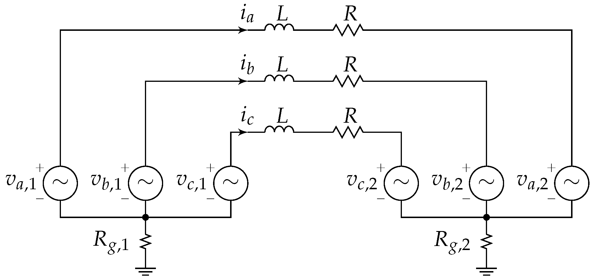
- Recall that balanced three-phase signals are sinusoidal signals with equal magnitudes, phase shifts of , and a sum of zero.
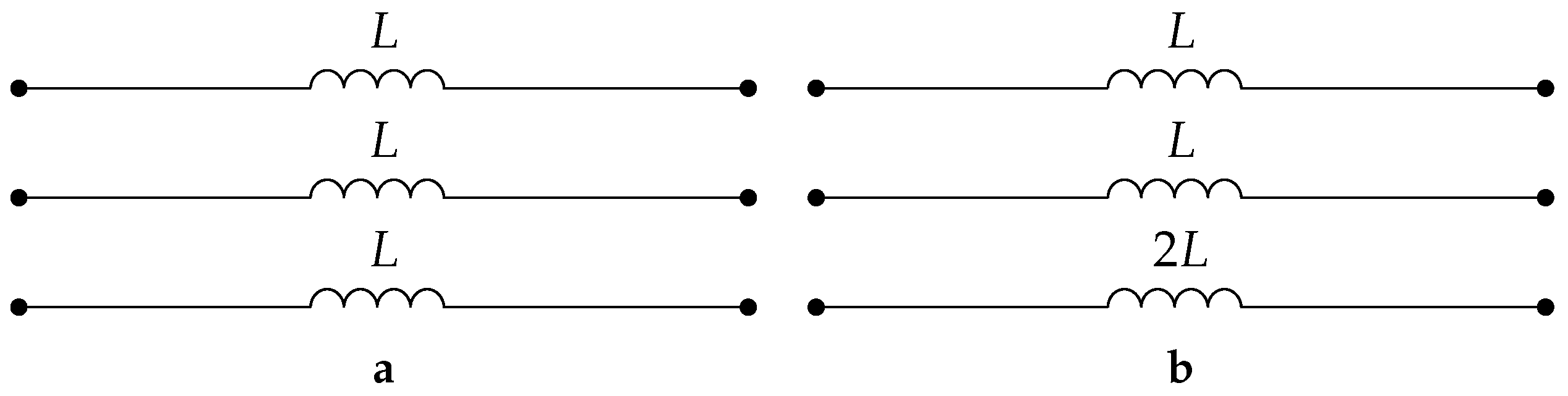
- We say that a power network is balanced or symmetrically configured if balanced three-phase voltages at its ports result in balanced three-phase currents, and vice versa. Two examples are shown in Figure 2.
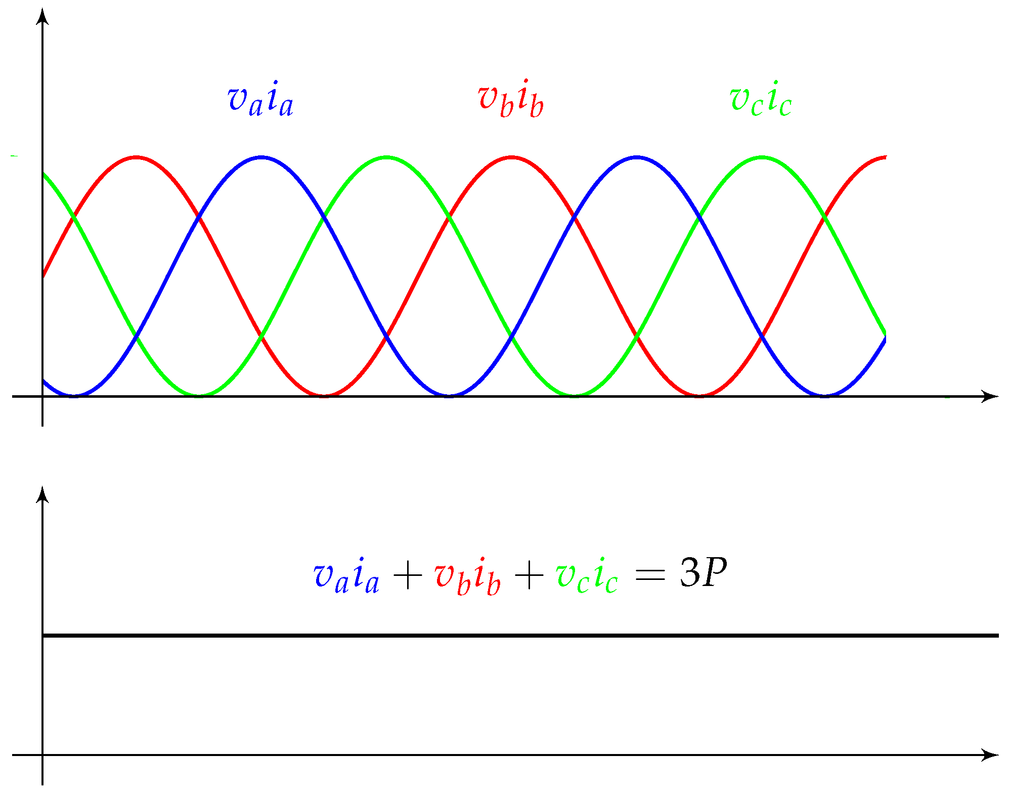
2.1.2. Power in Terms of DQ0 Quantities
2.1.3. Energy in Terms of DQ0 Quantities
2.2. Modeling General Linear Networks
2.3. Comparison of Time-Varying Phasors and DQ0 Models
2.4. Summary of Power Definitions
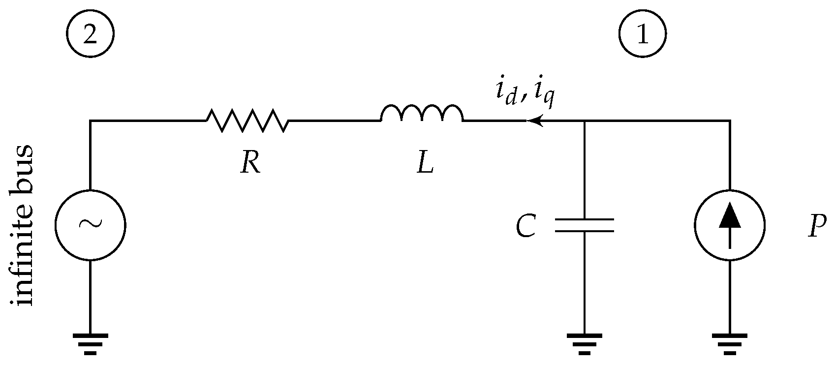
2.5. Example—Modeling a Network Based on DQ0 Quantities
- The network is symmetrically configured.
- The sources are balanced (equal amplitudes, between phases, ).
- Based on (61), the power source is defined bymeaning that under a quasi-static approximation the active power is P, and the reactive power is zero.
- The infinite bus has an RMS voltage of , and a frequency of .
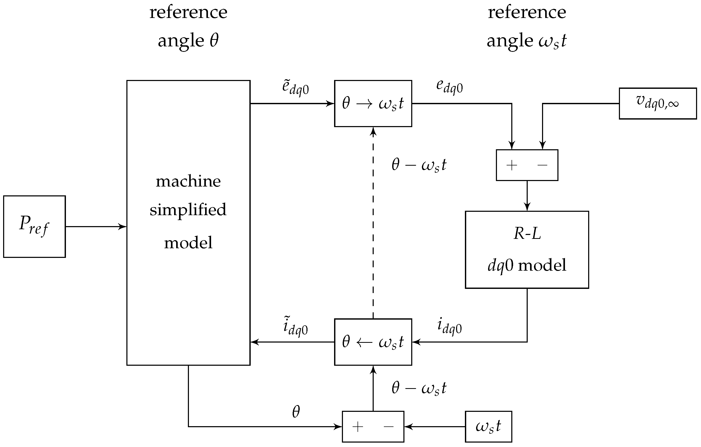
- We use a transformation with a reference angle .
- If , there is a pole in the right half of the complex plane, and the system is unstable.
- If , there is a complex conjugate pair of poles on the imaginary axis, and additional analysis in simulation reveals that the system is unstable.
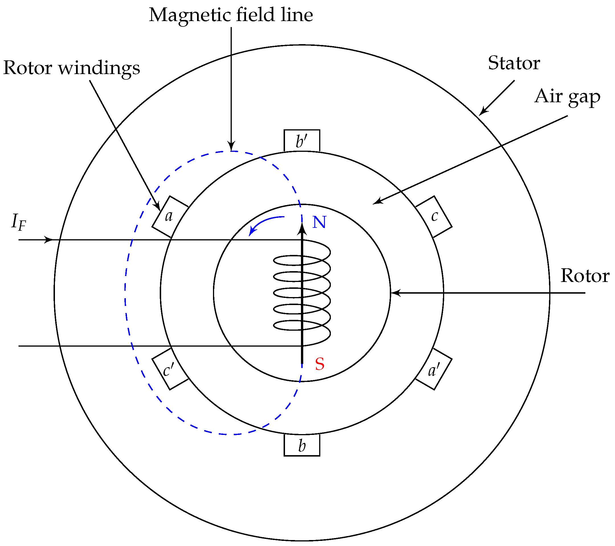
3. The Synchronous Machine
3.1. Mechanical and Electrical Angles
- is the rotor electrical angle, with respect to a fixed point on the stator.
- is the rotor mechanical angle, with respect to a fixed point on the stator.
- “poles” is the number of magnetic poles on the rotor (must be even).
3.2. Basic Mechanical Equations
3.3. Electrical Equations
- The machine is a magneto-quasi-static device.
- Saturation of the magnetic materials and other sources of imbalance and harmonic distortion are ignored.
- Self- and mutual inductances are composed of a constant term, in addition to a sinusoidal term varying with .
- , , are stator flux linkages.
- , , are the stator currents (generator output currents). The negative signs have been added since currents are positive when flowing out of the generator.
- is field winding flux linkage.
- is field winding current.
- , , are the stator voltages (generator output voltages).
- is the field winding voltage.
- is the armature resistance.
- is the field winding resistance.
- , , are the transformation of , , (stator voltages).
- , , are the transformation of , , (stator flux linkages).
- is called the direct-axis synchronous inductance.
- is called the quadrature-axis synchronous inductance.
- is called the zero-sequence inductance.
- The reference angle for the transformation is the rotor electrical angle .
- The variables do not depend directly on , and define a time-invariant model.
3.4. Simplified Machine Model
- Round rotor: , or equivalently .
- Constant field current: .
- Balanced voltages and currents: , .
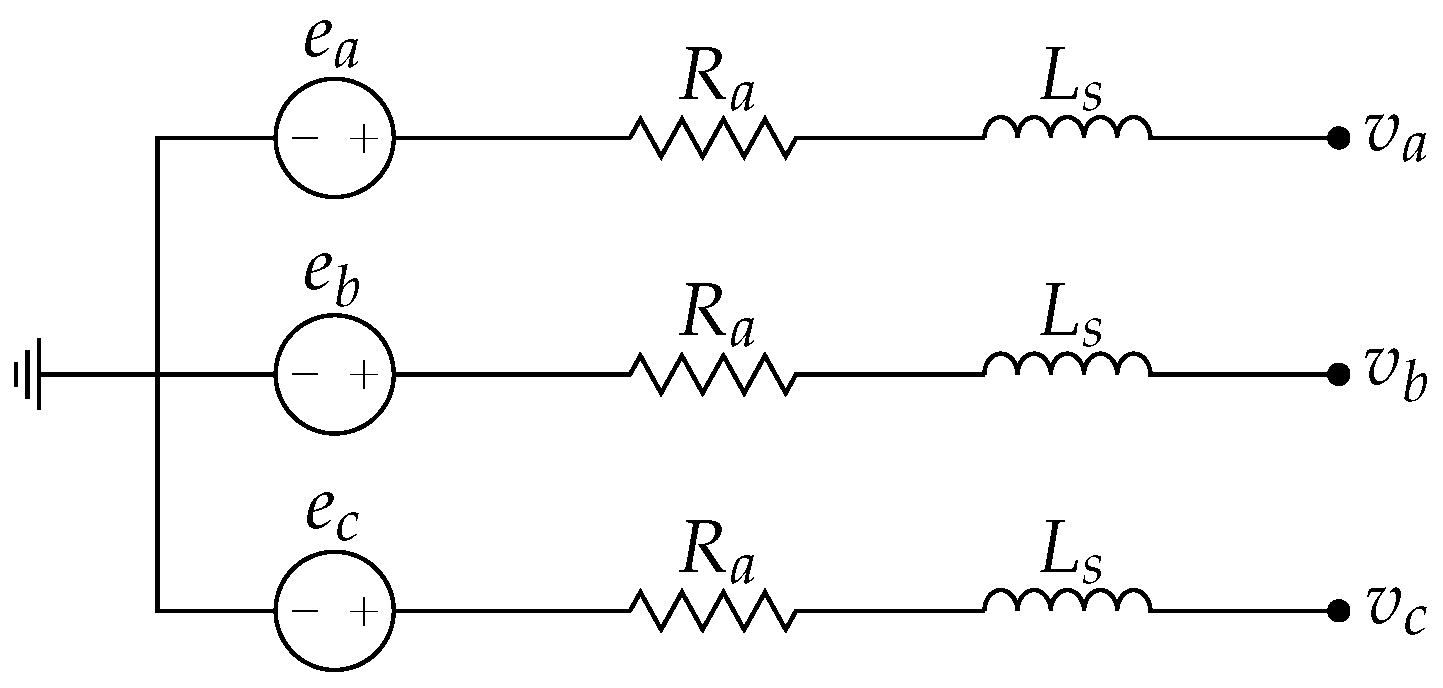
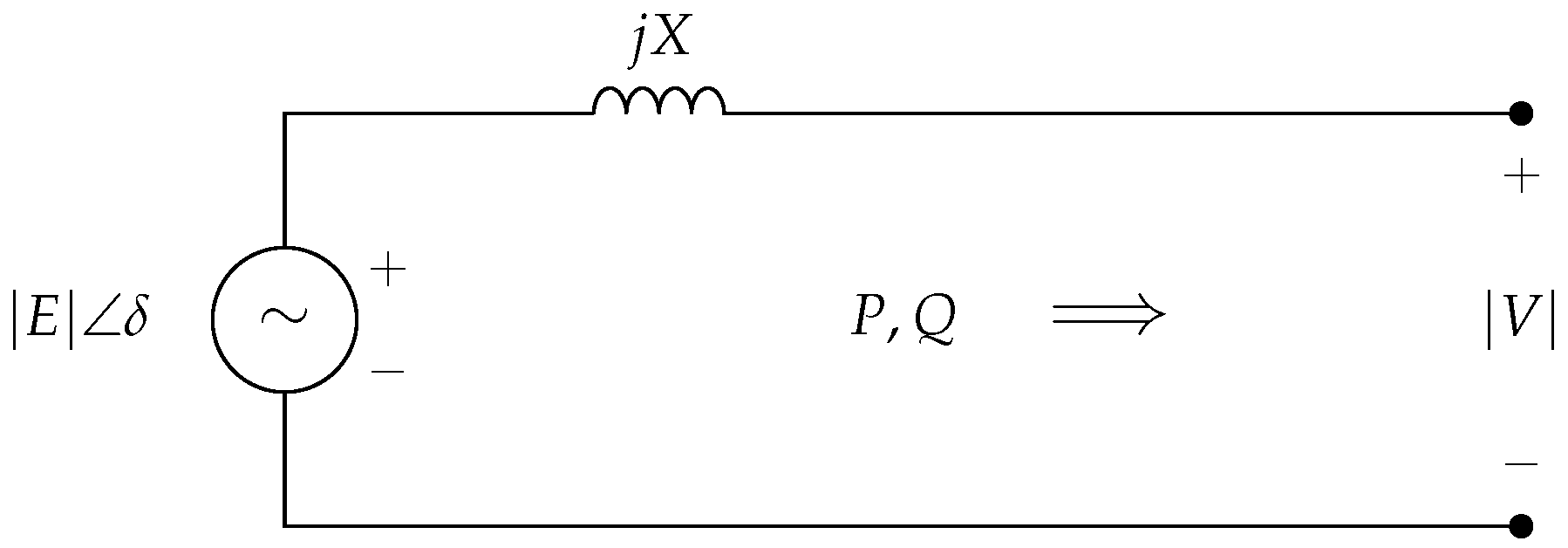
- The machine may be described as an EMF source behind a series impedance.
- The EMF is proportional to the frequency .
- The electric torque is proportional to the current .
- The induced EMF is proportional to the frequency, where at steady-state and at nominal frequency the induced EMF (peak value) is .
- The induced EMF is equal to the machine’s open-circuit voltage. This can be seen in Figure 13, assuming that the stator currents are zero.
3.5. Energy Conversion in the Machine
- The kinetic energy of the rotor: .
- The magnetic energy, represented by the energy stored in the synchronous inductance: .
- is the electric power decelerating the rotor. This is also the power generated by the EMF source, as shown below.
- is the machine’s output power.
- is the ohmic power loss on the armature resistance.
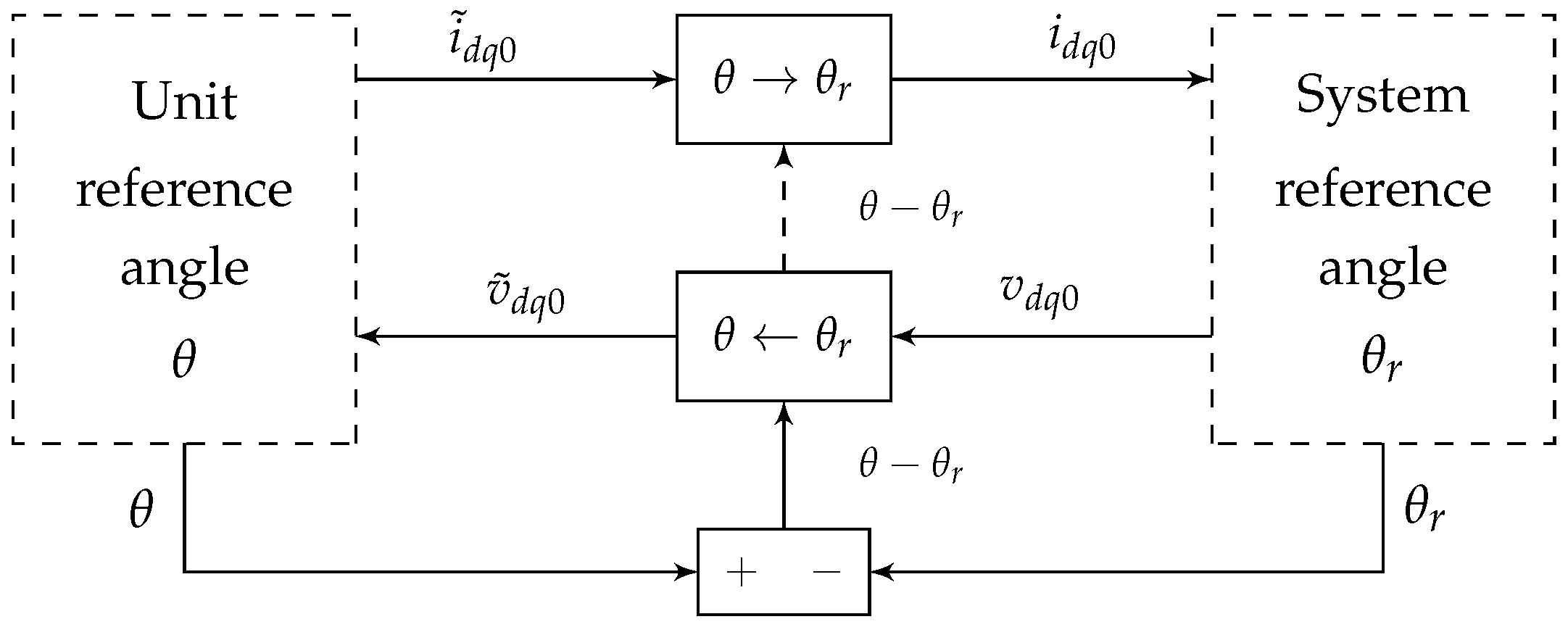
3.6. Transformation from One Reference Frame to Another
4. Three-Phase Inverters
4.1. Basic Definitions
- The frequency .
- The (single-phase) active power P, such that .
- The (single-phase) reactive power Q.
- The voltage amplitude .
- The voltage angle .
4.2. Modes of Operation
4.2.1. Grid Forming Inverters
4.2.2. Grid Feeding Inverters
4.2.3. Grid Supporting Inverters
4.3. Grid Forming Inverters
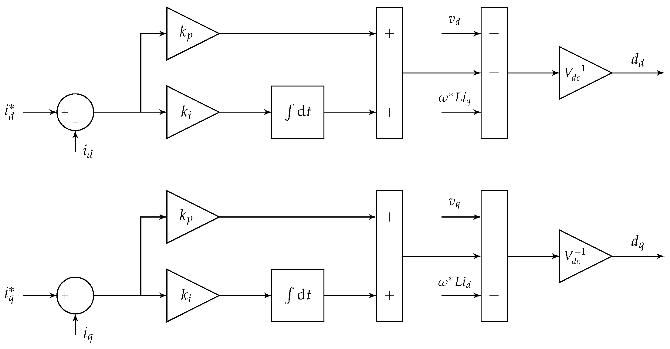
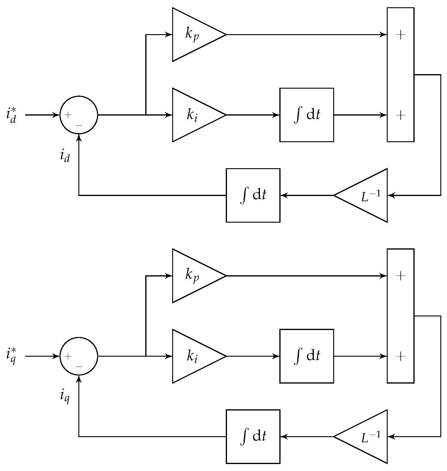
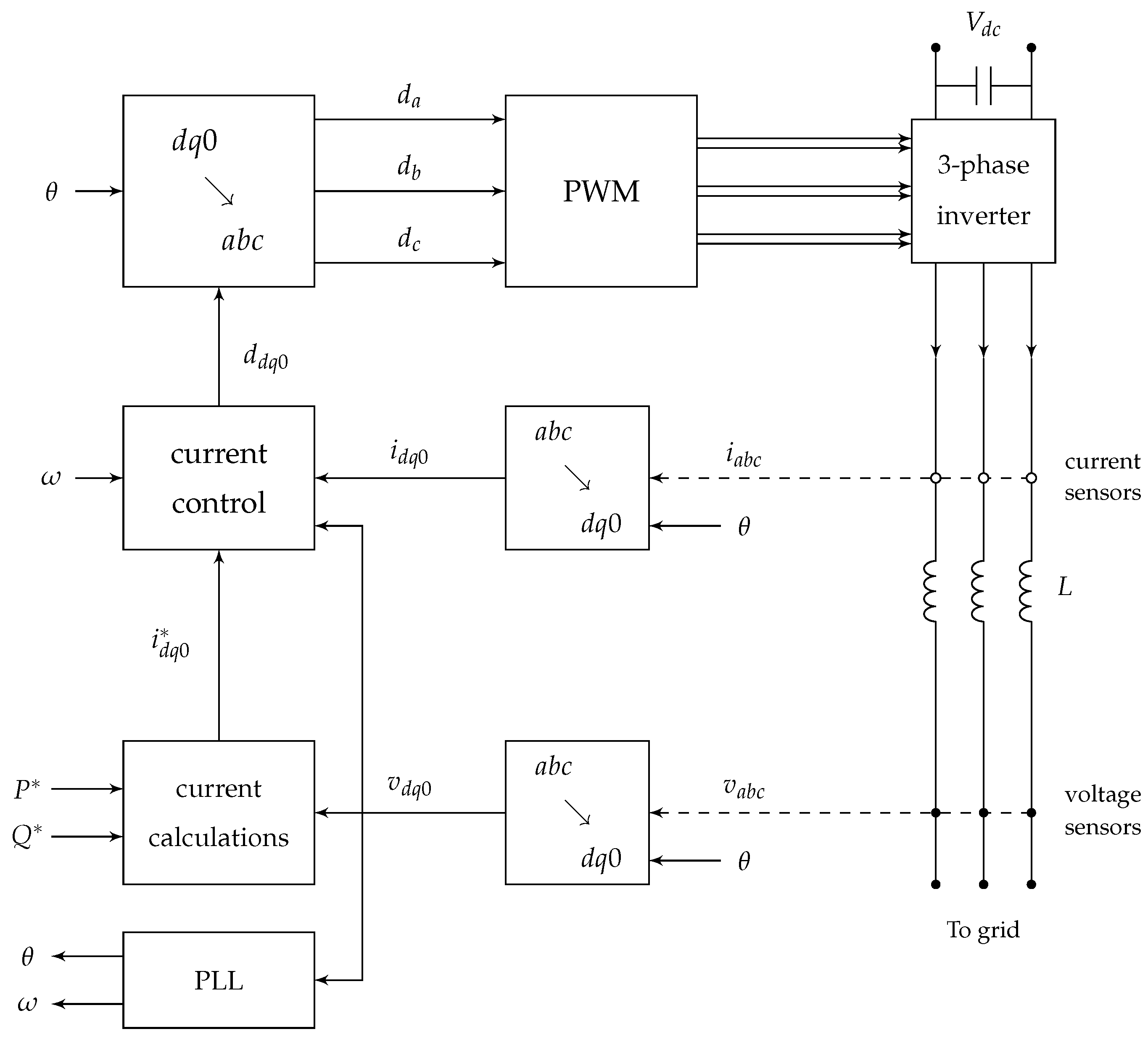
4.4. Grid Feeding Inverters
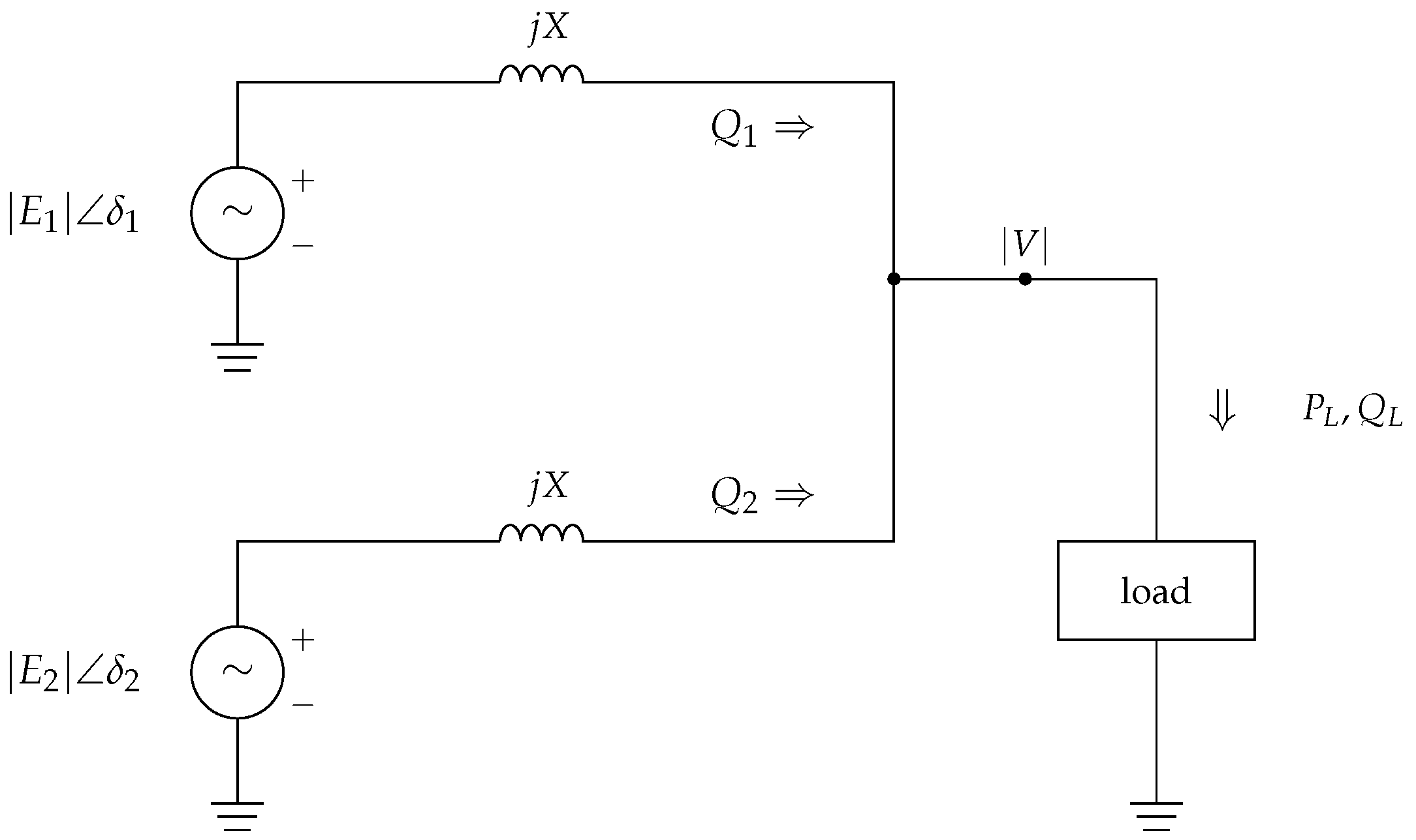
4.5. Droop Control
- Regulate the frequency and active power.
- Regulate the voltage and reactive power.
- Promote fair sharing of active power among generators.
- Promote fair sharing of reactive power among generators.
- Allow generators of different sizes to operate in parallel.
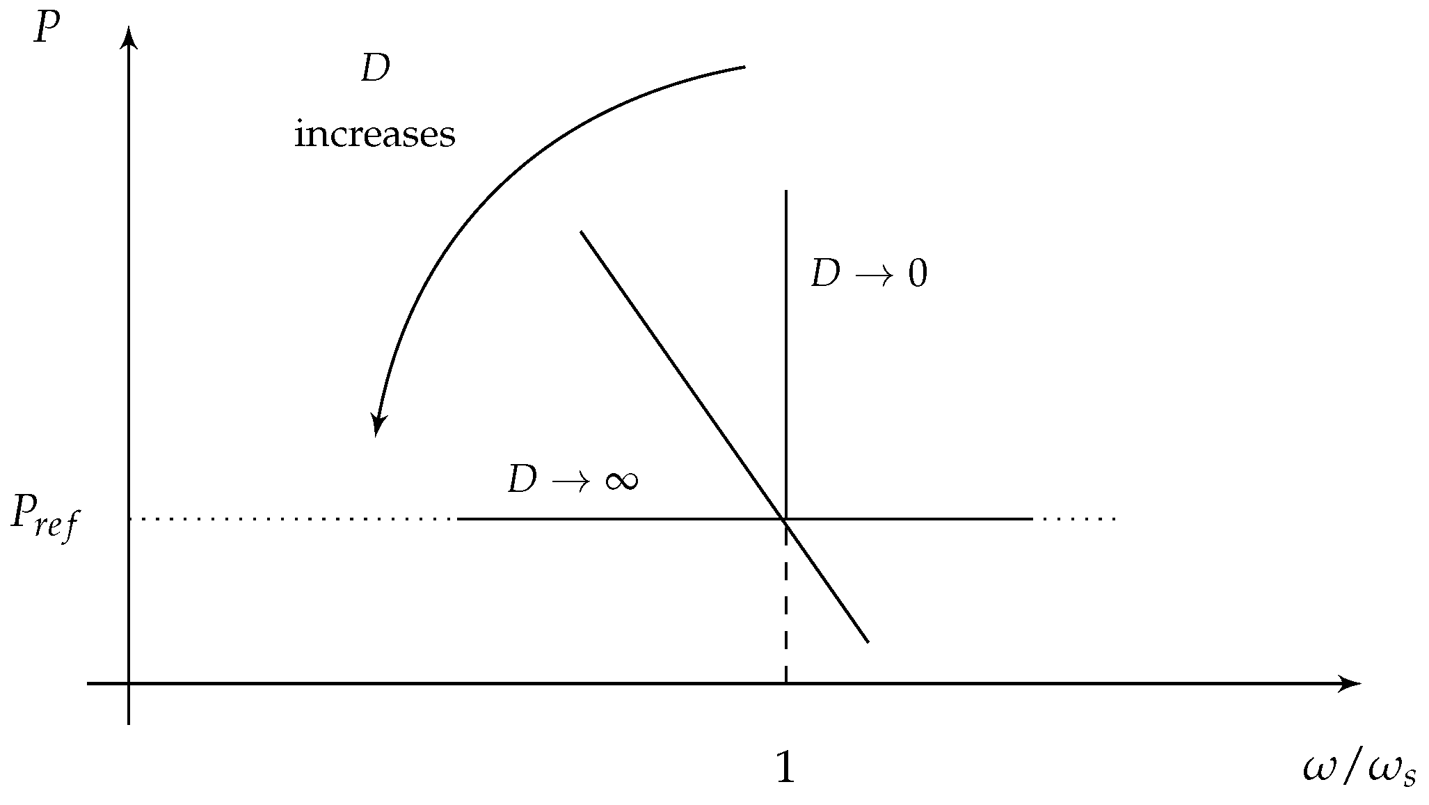
4.5.1. Frequency Droop Control
- The frequency is constant such that . The generator provides active power as needed to stabilize the frequency.
- The active power varies.
- The generator operates like a grid forming inverter, or an infinite bus.
- The active power is constant, .
- The frequency varies.
- The generator operates as a power source, like a grid feeding inverter.
- Combine the properties of these two extreme cases.
- The active power is regulated, but is not constant. The generator provides variable active power to adjust the frequency.
- The frequency is regulated, but is not constant.
- As we shall see, the generator operates like a grid supporting inverter.
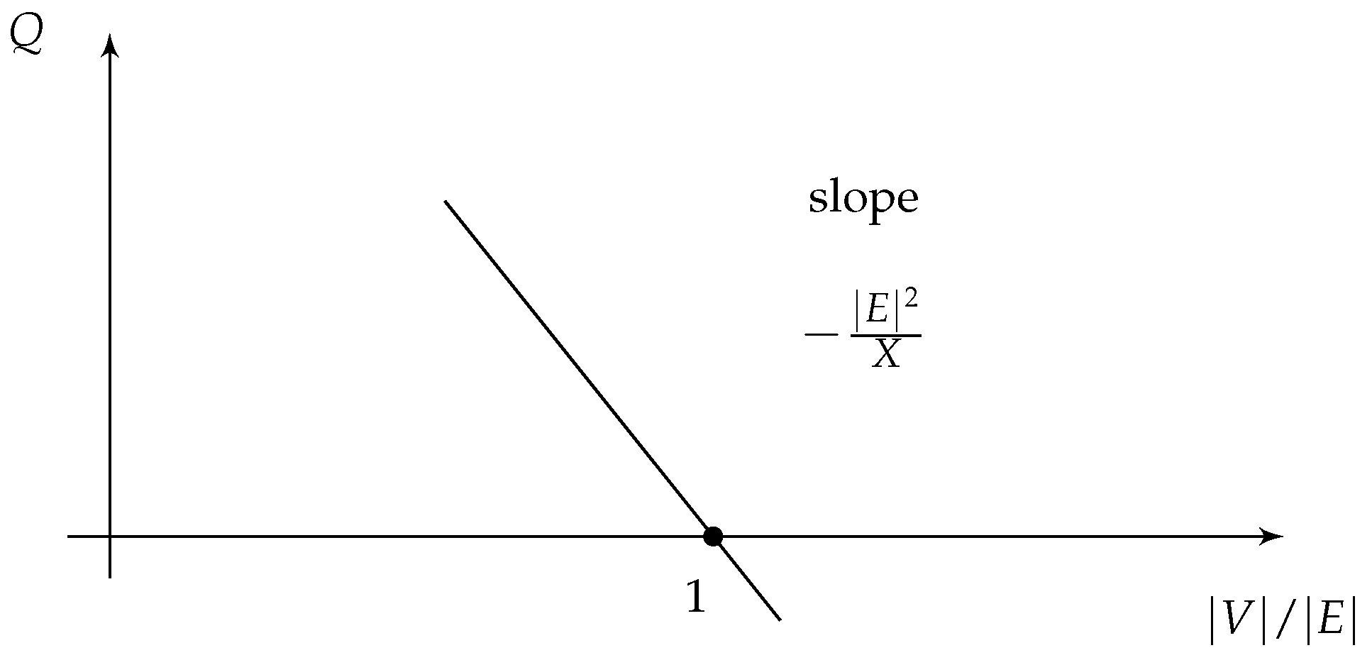
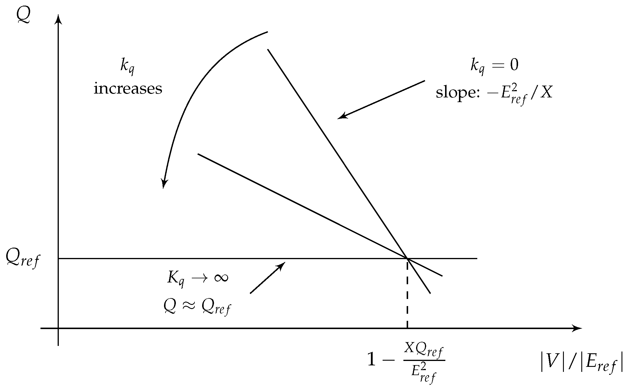
4.5.2. Voltage Droop Control
- The voltage varies in a small range. The generator provides reactive power as needed to maintain a certain voltage amplitude. As decreases, the reactive power increases to compensate.
- The reactive power varies.
- The generator operates as a voltage source, or like a grid forming inverter.
- The reactive power is regulated, .
- The voltage varies.
- The generator operates as a power source, or like a grid feeding inverter.
- Combine the properties of these two extreme cases.
- The reactive power is regulated, but is not constant.
- The voltage is somewhat regulated. The generator provides reactive power to maintain a stable voltage.
- As we shall see, the generator operates like a grid supporting inverter.
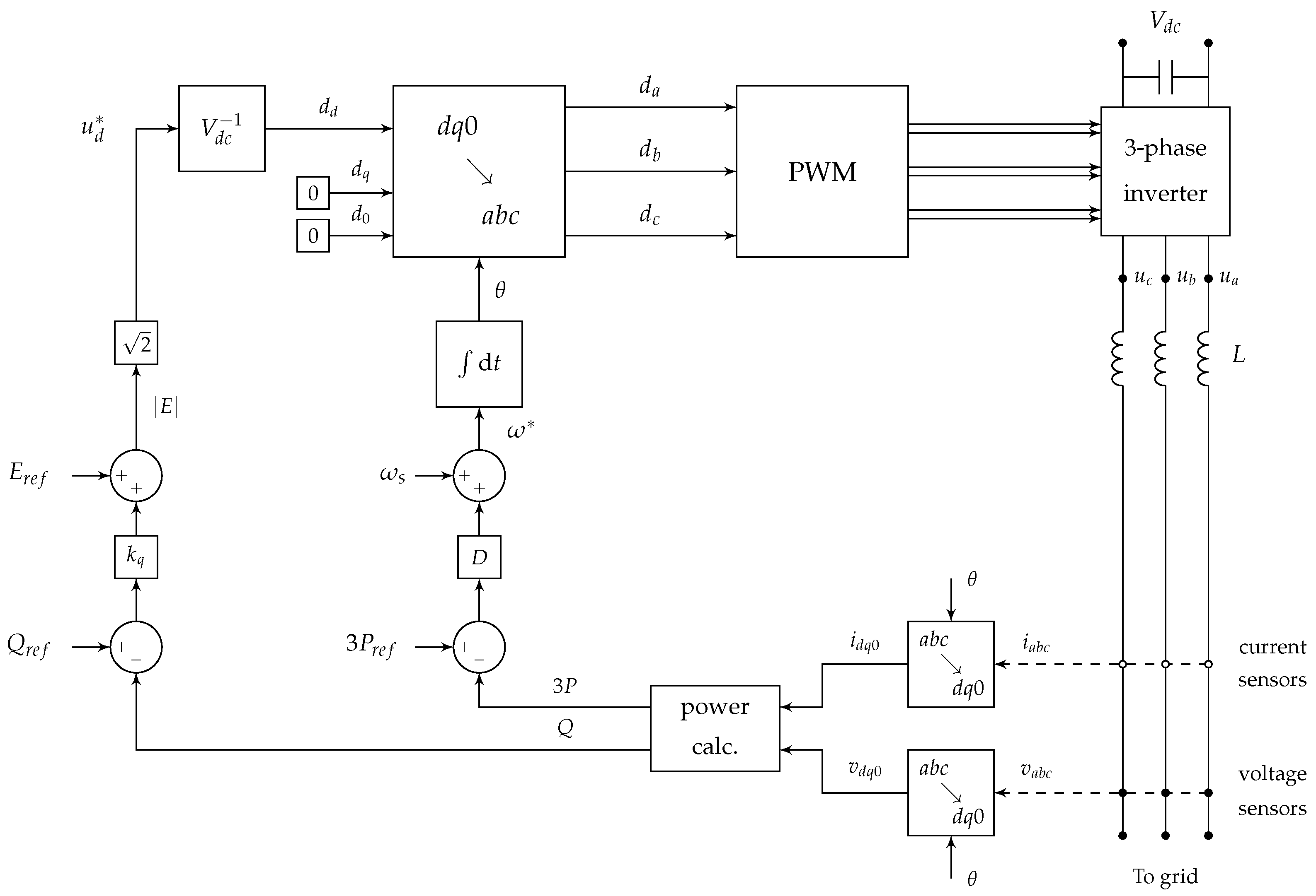
4.6. Grid Supporting Inverters
- If , then the frequency is constant , as in grid forming inverters.
- If , then the active power is constant , as in grid feeding inverters.
- If , then the voltage amplitude is constant , as in grid forming inverters.
- If , then the reactive power is constant , as in grid feeding inverters.
- Middle values: the inverter supports the grid by regulating the active power, reactive power, frequency and voltage.
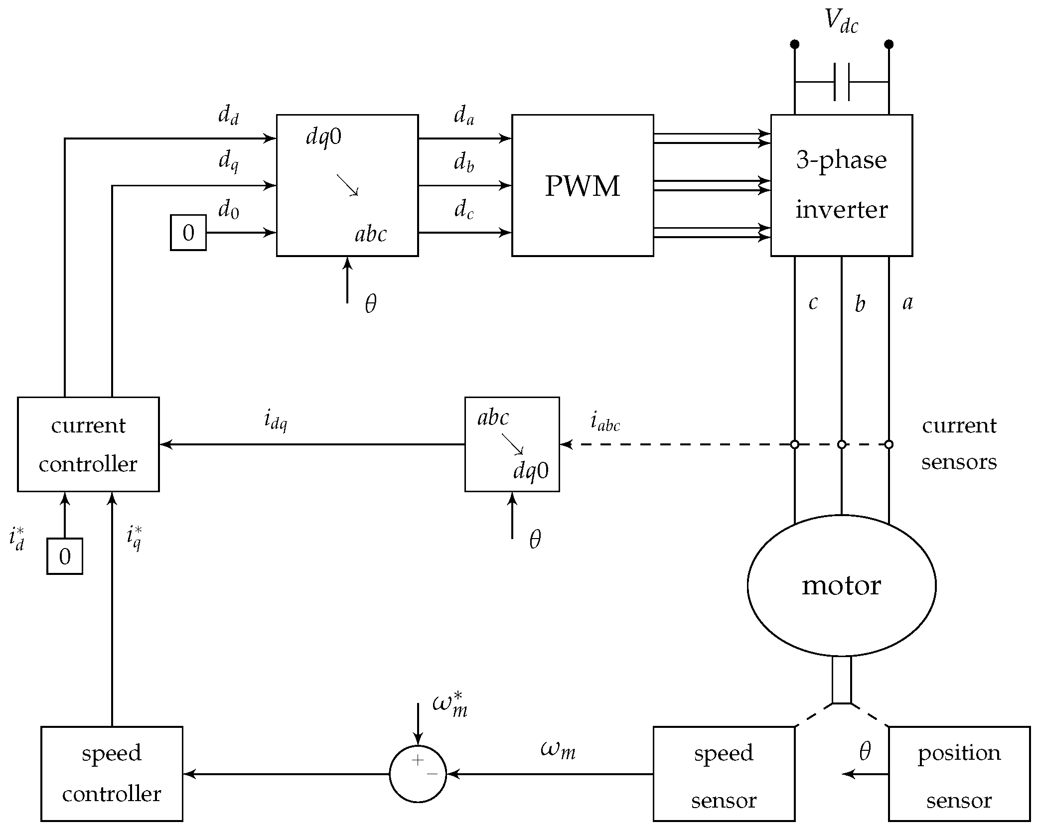
4.7. Control of PMSM
- The stator currents are defined positive when flowing into the machine.
- The term is replaced with , which is the amplitude of the flux induced in the stator phases by the permanent magnets on the rotor.
- The electromagnetic torque accelerates the rotor, and the mechanical torque decelerates the rotor. The angular acceleration is defined as .
- is the rotor electrical angle, measured with respect to a fixed point on the stator;
- is the number of pole pairs;
- , , are the direct-axis, quadrature-axis, and zero-sequence inductances;
- R is the resistance of the stator windings;
- , , are the stator currents (positive when flowing into the machine);
- , , are the stator voltages;
- is the angular velocity of the rotor;
- is the amplitude of the flux induced in the stator phases by the permanent magnets on the rotor;
- J is the rotor moment of inertia;
- , are the mechanical and electromagnetic torques;
- , are the mechanical and electromagnetic powers.
5. Conclusions
Author Contributions
Funding
Acknowledgments
Conflicts of Interest
Appendix A. Useful DQ0 Identities
Appendix B. The Synchronous Machine
Appendix B.1. Summary of Symbols and Definitions

| “poles”–number of magnetic poles on the rotor (must be even) | –rotor electrical angle, with respect to a fixed point on the stator | –induced EMF at steady state and at nominal frequency, peak value |
| J–rotor moment of inertia | –rotor electrical frequency [rad/s] | – induced EMF at steady state and at the rotor frequency, RMS value |
| D–damping factor | –rotor mechanical frequency [rad/s] | , , –stator currents (generator output currents) |
| , –direct axis and quadrature axis synchronous inductances | –nominal grid frequency [rad/s]. For instance, or rad/s | , , –stator currents (generator output voltages) |
| –zero sequence inductance | –mechanical torque (accelerating the rotor for generator) | –swing equation constant |
| synchronous inductance | –electric torque (decelerating the rotor for generator) | , , –induced EMF in the simplified machine model |
| –stator to rotor mutual inductance (maximum value) | –reference power for droop control. This is the single phase output power at steady state and at nominal frequency (losses neglected) | –field winding voltage |
| –field winding self-inductance | –mechanical power (total for 3-phase) | –field winding current |
| –armature resistance | –electrical power (total for 3-phase) | , , –stator flux linkages |
| –field winding resistance | –machine output power (total for the 3 phases) | –field winding flux linkage |
Appendix B.2. Default Values
- or [rad/s] is the nominal grid frequency.
- “poles” is the number of magnetic poles on the rotor (default is poles = 2).
- [W] is the machine rated power (maximum power for a single phase).
- [W] is the reference power for the droop control. This is the single-phase output power of the machine at steady state, and at nominal frequency (losses neglected). This parameter usually equals to a fraction of , for instance . This value may change during normal operation.
- [Vrms] is the machine rated voltage, RMS value (induced EMF at nominal frequency).
| Inertia constant | s | |
| rotor moment of inertia | ||
| droop-control damping factor | ||
| direct axis synchronous inductance | H | |
| quadrature axis synchronous inductance | H | |
| synchronous inductance | H | |
| zero sequence inductance | H | |
| armature resistance | ||
| stator to rotor mutual inductance (maximum value) | H | |
| field winding self-inductance | H | |
| field winding resistance | ||
| field winding current (default DC value) | A | |
| field winding voltage (default DC value) | V | |
| constant used in the detailed model | H2 | |
| swing equation constant |
References
- Moeini, A.; Kamwa, I.; Brunelle, P.; Sybille, G. Open data IEEE test systems implemented in SimPowerSystems for education and research in power grid dynamics and control. In Proceedings of the 50th International Universities Power Engineering Conference, Stoke on Trent, UK, 1–4 September 2015; pp. 1–6. [Google Scholar]
- Anderson, P.M.; Fouad, A.A. Power System Control and Stability; John Wiley & Sons: Hoboken, NJ, USA, 2008. [Google Scholar]
- Kundur, P. Power System Stability and Control; McGraw-Hill: New York, NY, USA, 1994. [Google Scholar]
- Kundur, P.; Paserba, J.; Ajjarapu, V.; Andersson, G.; Bose, A.; Canizares, C.; Hatziargyriou, N.; Hill, D.; Stankovic, A.; Taylor, C.; et al. Definition and classification of power system stability IEEE/CIGRE joint task force on stability terms and definitions. IEEE Trans. Power Syst. 2004, 19, 1387–1401. [Google Scholar]
- Miller, L.; Cibulka, L.; Brown, M.; von Meier, A. Electric Distribution System Models for Renewable Integration: Status and Research Gaps Analysis; Technical Report CEC-500-10-055; California Energy Commission: Sacramento, CA, USA, 2013.
- Grainger, J.J.; Stevenson, W.D. Power System Analysis; McGraw-Hill: New York, NY, USA, 1994. [Google Scholar]
- Ilić, M.; Zaborszky, J. Dynamics and Control of Large Electric Power Systems; Chapter Quasistationary Phasor Concepts; Wiley: New York, NY, USA, 2000; pp. 9–60. [Google Scholar]
- Sauer, P.W.; Pai, M.A. Power System Dynamics and Stability; Prentice Hall: Upper Saddle River, NJ, USA, 1998. [Google Scholar]
- Ilić, M.; Jaddivada, R.; Miao, X. Modeling and analysis methods for assessing stability of microgrids. IFAC-PapersOnLine 2017, 50, 5448–5455. [Google Scholar] [CrossRef]
- Demiray, T.H. Simulation of Power System Dynamics Using Dynamic Phasor Models. Ph.D. Thesis, TU Wien, Wien, Austria, June 2008. [Google Scholar]
- Belikov, J.; Levron, Y. Comparison of time-varying phasor and dq0 dynamic models for large transmission networks. Int. J. Electr. Power 2017, 93, 65–74. [Google Scholar] [CrossRef]
- Belikov, J.; Levron, Y. Uses and misuses of quasi-static models in modern power systems. IEEE Trans. Power Deliv. 2018. Available online: https://ieeexplore.ieee.org/document/8403297/ (accessed on 14 September 2018). [CrossRef]
- Krause, P.C.; Wasynczuk, O.; Sudhoff, S.D.; Pekarek, S. Analysis of Electric Machinery and Drive Systems, 3rd ed.; Wiley-IEEE Press: Piscataway, NJ, US, 2013. [Google Scholar]
- Machowski, J.; Bialek, J.; Bumby, J. Power Dystem Dynamics: Stability and Control; John Wiley & Sons: Hoboken, NJ, USA, 2011. [Google Scholar]
- Fasil, M.; Antaloae, C.; Mijatovic, N.; Jensen, B.B.; Holboll, J. Improved dq-axes model of PMSM considering airgap flux harmonics and saturation. IEEE Trans. Appl. Supercond. 2016, 26, 1–5. [Google Scholar] [CrossRef]
- Adhikari, S.; Li, F.; Li, H. P-Q and P-V control of photovoltaic generators in distribution systems. IEEE Trans. Smart Grids 2015, 6, 2929–2941. [Google Scholar] [CrossRef]
- Buccella, C.; Cecati, C.; Latafat, H.; Razi, K. Multi string grid-connected PV system with LLC resonant DC/DC converter. Int. Ind. Syst. 2015, 1, 37–49. [Google Scholar] [CrossRef]
- Jafari, A.; Shahgholian, G. Analysis and simulation of a sliding mode controller for mechanical part of a doubly-fed induction generator based wind turbine. IET Gener. Transm. Dis. 2017, 11, 2677–2688. [Google Scholar] [CrossRef]
- Njiri, J.G.; Söffker, D. State-of-the-art in wind turbine control: Trends and challenges. Renew. Sustain. Energy Rev. 2016, 60, 377–393. [Google Scholar] [CrossRef]
- Schiffer, J.; Zonetti, D.; Ortega, R.; Stanković, A.M.; Sezi, T.; Raisch, J. A survey on modeling of microgrids—From fundamental physics to phasors and voltage sources. Automatica 2016, 74, 135–150. [Google Scholar] [CrossRef]
- Mahmoud, M.S.; Hussainr, S.A.; Abido, M.A. Modeling and control of microgrid: An overview. J. Frankl. Inst. 2014, 351, 2822–2859. [Google Scholar] [CrossRef]
- Ojo, Y.; Schiffer, J. Towards a time-domain modeling framework for small-signal analysis of unbalanced microgrids. In Proceedings of the 12th IEEE PES PowerTech Conference, Manchester, UK, 18–22 June 2017; pp. 1–6. [Google Scholar]
- Belikov, J.; Levron, Y. A sparse minimal-order dynamic model of power networks based on dq0 signals. IEEE Trans. Power Syst. 2018, 33, 1059–1067. [Google Scholar] [CrossRef]
- Levron, Y.; Belikov, J. Modeling power networks using dynamic phasors in the dq0 reference frame. Electr. Power Syst. Res. 2017, 144, 233–242. [Google Scholar] [CrossRef]
- Baimel, D.; Belikov, J.; Guerrero, J.M.; Levron, Y. Dynamic modeling of networks, microgrids, and renewable sources in the dq0 reference frame: A survey. IEEE Access 2017, 5, 21323–21335. [Google Scholar] [CrossRef]
- Demiray, T.; Andersson, G. Comparison of the efficiency of dynamic phasor models derived from ABC and DQ0 reference frame in power system dynamic simulations. In Proceedings of the 7th IET International Conference on Advances in Power System Control, Operation and Management, Hong Kong, China, 30 October–2 November 2006; pp. 1–8. [Google Scholar]
- Stefanov, P.C.; Stanković, A.M. Modeling of UPFC operation under unbalanced conditions with dynamic phasors. IEEE Trans. Power Syst. 2002, 17, 395–403. [Google Scholar] [CrossRef]
- Fitzgerald, A.E.; Kingsley, C.; Umans, S.D. Electric Machinery, 6th ed.; McGraw-Hill: New York, NY, USA, 2003. [Google Scholar]
- Teodorescu, R.; Liserre, M.; Rodriguez, P. Grid Converters for Photovoltaic and Wind Power Systems; John Wiley & Sons: Hoboken, NJ, USA, 2011. [Google Scholar]
- Belikov, J.; Levron, Y. Integration of long transmission lines in large-scale dq0 dynamic models. Electr. Eng. 2018, 100, 1219–1228. [Google Scholar] [CrossRef]
- Kwon, W.H.; Cho, G.H. Analyses of static and dynamic characteristics of practical step-up nine-switch matrix convertor. IEE Proc. B Electr. Power Appl. 1993, 140, 139–146. [Google Scholar] [CrossRef]
- Szcześniak, P.; Fedyczak, Z.; Klytta, M. Modelling and analysis of a matrix-reactance frequency converter based on buck-boost topology by DQ0 transformation. In Proceedings of the 13th International Power Electronics and Motion Control Conference, Poznan, Poland, 1–3 September 2008; pp. 165–172. [Google Scholar]
- Fahima, A.; Ofir, R.; Belikov, J.; Levron, Y. Minimal energy storage required for stability of low inertia distributed sources. In Proceedings of the 2018 IEEE International Energy Conference (ENERGYCON), Limassol, Cyprus, 3–7 June 2018; pp. 1–5. [Google Scholar]
- Rocabert, J.; Luna, A.; Blaabjerg, F.; Rodríguez, P. Control of power converters in AC microgrids. IEEE Trans. Power Electron. 2012, 27, 4734–4749. [Google Scholar] [CrossRef]
- Wang, X.; Guerrero, J.M.; Blaabjerg, F.; Chen, Z. A review of power electronics based microgrids. J. Power Electron. 2012, 12, 181–192. [Google Scholar] [CrossRef]
- Dou, X.; Yang, K.; Quan, X.; Hu, Q.; Wu, Z.; Zhao, B.; Li, P.; Zhang, S.; Jiao, Y. An optimal PR control strategy with load current observer for a three-phase voltage source inverter. Energies 2015, 8, 7542–7562. [Google Scholar] [CrossRef]
- Loh, P.C.; Holmes, D.G. Analysis of multiloop control strategies for LC/CL/LCL-filtered voltage-source and current-source inverters. IEEE Trans. Ind. Appl. 2005, 41, 644–654. [Google Scholar] [CrossRef]
- Mohamed, Y.A.R.I.; El-Saadany, E.F. A control method of grid-connected PWM voltage source inverters to mitigate fast voltage disturbances. IEEE Trans. Power Syst. 2009, 24, 489–491. [Google Scholar] [CrossRef]
- Pogaku, N.; Prodanovic, M.; Green, T.C. Modeling, analysis and testing of autonomous operation of an inverter-based microgrid. IEEE Trans. Power Electron. 2007, 22, 613–625. [Google Scholar] [CrossRef]
- Serban, I.; Ion, C.P. Microgrid control based on a grid-forming inverter operating as virtual synchronous generator with enhanced dynamic response capability. Int. J. Electr. Power 2017, 89, 94–105. [Google Scholar] [CrossRef]
- Teodorescu, R.; Blaabjerg, F.; Liserre, M.; Loh, P.C. Proportional-resonant controllers and filters for grid-connected voltage-source converters. IEE P.-Electr. Power Appl. 2006, 153, 750–762. [Google Scholar] [CrossRef]
- Zhang, T.; Yue, D.; O’Grady, M.J.; O’Hare, G.M.P. Transient oscillations analysis and modified control strategy for seamless mode transfer in micro-grids: A wind-PV-ES hybrid system case study. Energies 2015, 8, 13758–13777. [Google Scholar] [CrossRef]
- Zhong, Q.C.; Hornik, T. Control of Power Inverters in Renewable Energy and Smart Grid Integration; John Wiley & Sons: New York, NY, USA, 2013. [Google Scholar]
- Bolognani, S.; Zampieri, S. A distributed control strategy for reactive power compensation in smart microgrids. IEEE Trans. Autom. Control 2013, 58, 2818–2833. [Google Scholar] [CrossRef]
- Cao, H.; Zhang, H.; Jiang, W.; Wei, S. Research on PQ control strategy for PV inverter in the unbalanced grid. In Proceedings of the Asia-Pacific Power and Energy Engineering Conference, Shanghai, China, 27–29 March 2012; pp. 1–3. [Google Scholar]
- Hans, C.A.; Nenchev, V.; Raisch, J.; Reincke-Collon, C. Minimax model predictive operation control of microgrids. IFAC Proc. Vol. 2014, 47, 10287–10292. [Google Scholar] [CrossRef]
- Katiraei, F.; Iravani, R.; Hatziargyriou, N.; Dimeas, A. Microgrids management. IEEE Power Energy Mag. 2008, 6, 54–65. [Google Scholar] [CrossRef]
- Peças Lopes, J.A.; Moreira, C.L.; Madureira, A.G. Defining control strategies for microgrids islanded operation. IEEE Trans. Power Syst. 2006, 21, 916–924. [Google Scholar] [CrossRef]
- Piegari, L.; Tricoli, P. A control algorithm of power converters in smart-grids for providing uninterruptible ancillary services. In Proceedings of the 14th International Conference on Harmonics and Quality of Power, Bergamo, Italy, 26–29 September 2010; pp. 1–7. [Google Scholar]
- Schonardie, M.F.; Coelho, R.F.; Schweitzer, R.; Martins, D.C. Control of the active and reactive power using dq0 transformation in a three-phase grid-connected PV system. In Proceedings of the IEEE International Symposium on Industrial Electronics, Hangzhou, China, 28–31 May 2012; pp. 264–269. [Google Scholar]
- Bouzid, A.M.; Guerrero, J.M.; Cheriti, A.; Bouhamida, M.; Sicard, P.; Benghanem, M. A survey on control of electric power distributed generation systems for microgrid applications. Renew. Sustain. Energy Rev. 2015, 44, 751–766. [Google Scholar] [CrossRef]
- Rodriguez, P.; Candela, I.; Citro, C.; Rocabert, J.; Luna, A. Control of grid-connected power converters based on a virtual admittance control loop. In Proceedings of the 15th European Conference on Power Electronics and Applications, Lille, France, 2–6 September 2013; pp. 1–10. [Google Scholar]


| Model | Operating Point | Small-Signal | High Frequencies | Non-Symmetric Networks |
|---|---|---|---|---|
| time-varying phasors | √ | √ | X | X |
| X | X | √ | √ | |
| √ | √ | √ | X |
| Grid Forming |
|
| Grid Feeding |
|
| Grid Supporting |
|
© 2018 by the authors. Licensee MDPI, Basel, Switzerland. This article is an open access article distributed under the terms and conditions of the Creative Commons Attribution (CC BY) license (http://creativecommons.org/licenses/by/4.0/).
Share and Cite
Levron, Y.; Belikov, J.; Baimel, D. A Tutorial on Dynamics and Control of Power Systems with Distributed and Renewable Energy Sources Based on the DQ0 Transformation. Appl. Sci. 2018, 8, 1661. https://doi.org/10.3390/app8091661
Levron Y, Belikov J, Baimel D. A Tutorial on Dynamics and Control of Power Systems with Distributed and Renewable Energy Sources Based on the DQ0 Transformation. Applied Sciences. 2018; 8(9):1661. https://doi.org/10.3390/app8091661
Chicago/Turabian StyleLevron, Yoash, Juri Belikov, and Dmitry Baimel. 2018. "A Tutorial on Dynamics and Control of Power Systems with Distributed and Renewable Energy Sources Based on the DQ0 Transformation" Applied Sciences 8, no. 9: 1661. https://doi.org/10.3390/app8091661
APA StyleLevron, Y., Belikov, J., & Baimel, D. (2018). A Tutorial on Dynamics and Control of Power Systems with Distributed and Renewable Energy Sources Based on the DQ0 Transformation. Applied Sciences, 8(9), 1661. https://doi.org/10.3390/app8091661