Article

A New Method to Retrieve the Three-Dimensional Refractive Index and Specimen Size Using the Transport Intensity Equation, Taking Diffraction into Account

by
Marcel A. Agnero
1,2,*,
Kouakou Konan
1,
Alvarez T. Kossonou
1,
Olivier K. Bagui
1 and
Jérémie T. Zoueu
1
1
Laboratoire d’Instrumentation d’Image et Spectroscopie, Institut National Polytechnique Félix Houphouët-Boigny (INPH-B), BP 1093 Yamoussoukro, Cote D’Ivoire
2
Laboratoire de Physique de la Matière Condensée et Technologie, UFR SSMT, Université Félix Houphouët-Boigny, 22 BP 582 Abidjan 22, Cote D’Ivoire
*
Author to whom correspondence should be addressed.
Appl. Sci. 2018, 8(9), 1649; https://doi.org/10.3390/app8091649
Submission received: 3 September 2018 / Revised: 12 September 2018 / Accepted: 12 September 2018 / Published: 13 September 2018
(This article belongs to the Section Optics and Lasers)

Abstract

:
Refractive index retrieval is possible using the transport intensity equation (TIE), which presents advantages over interferometric techniques. The TIE method is valid only for paraxial ray assumptions. However, diffraction can nullify these TIE model assumptions. Therefore, the refractive index is problematic for reconstruction in three-dimensions (3D) using a set of defocused images, as diffraction effects become prominent. We propose a method to recover the 3D refractive index by combining TIE and deconvolution. A brightfield (BF) microscope was then constructed to apply the proposed technique. A microsphere was used as a sample with well-known properties. The deconvolution of the BF-images of the sample using the microscope’s 3D point spread function led to significantly reduced diffraction effects. TIE was then applied for each set of three images. Applying TIE without taking into account diffraction failed to reconstruct the 3D refractive index. Taking diffraction into account, the refractive index of the sample was clearly recovered, and the sectioning effect of the microsphere was highlighted, leading to a determination of its size. This work is of great significance in improving the 3D reconstruction of the refractive index using the TIE method.

1. Introduction

Spectroscopic analysis of microscopic specimens sometimes requires knowledge of their refractive indices. The refractive index is an important biophysical parameter, which is used in many studies. In mineralogy and crystallography [1], the refractive index is taken into account in the characterization of precious stones. In medicine, it can be used as a marker of disease. Zhuo et al. [2] showed that it is possible to diagnose tissue cancers via the refractive index distribution, which contains information about the molecular scale organization of tissue. The refractive index maps of red blood cells are used as an indicator of the morphological alterations of host cells infected by Plasmodium falciparum [3].
Standard devices for the refractive index measurement lead to mean values of this important parameter. Progress is being made in the development of new devices and methods that enable the determination of the refractive index in three-dimensions (3D). These methods should help to raise the accuracy of specimen analysis. The most well-established methods for recovering the quantitative phase and the optical parameters are the interferometric method, such as digital holography. Using this method, Florian et al. [4] performed a 3D reconstruction of refractive index of pollen grain, with a precision of 0.01. The interferometric method needs coherent illumination. Therefore, it induces speckle noise in the measurements, which prevent high quality results [5]. Phase or refractive index retrieval is possible by using the Transport Intensity Equation (TIE) which is a non-interferometric method [6]. TIE has been increasingly investigated over recent years due to its unique advantages over interferometric techniques. It uses partially coherent illumination; it is computationally simple with the need of (at least) three brightfield (BF) defocused images, and it does not require a complicated optical system. However, the TIE method is valid only for paraxial ray approximations [7], and diffraction can nullify these TIE model assumptions. This phenomenon drastically affects the quality of the 3D reconstruction of the refractive index [8] as the diffraction effects become prominent.
In this work, we introduce a method to clearly recover the 3D refractive index of a sample with well-known properties by using TIE and taking the diffraction into account.

2. Materials and Methods

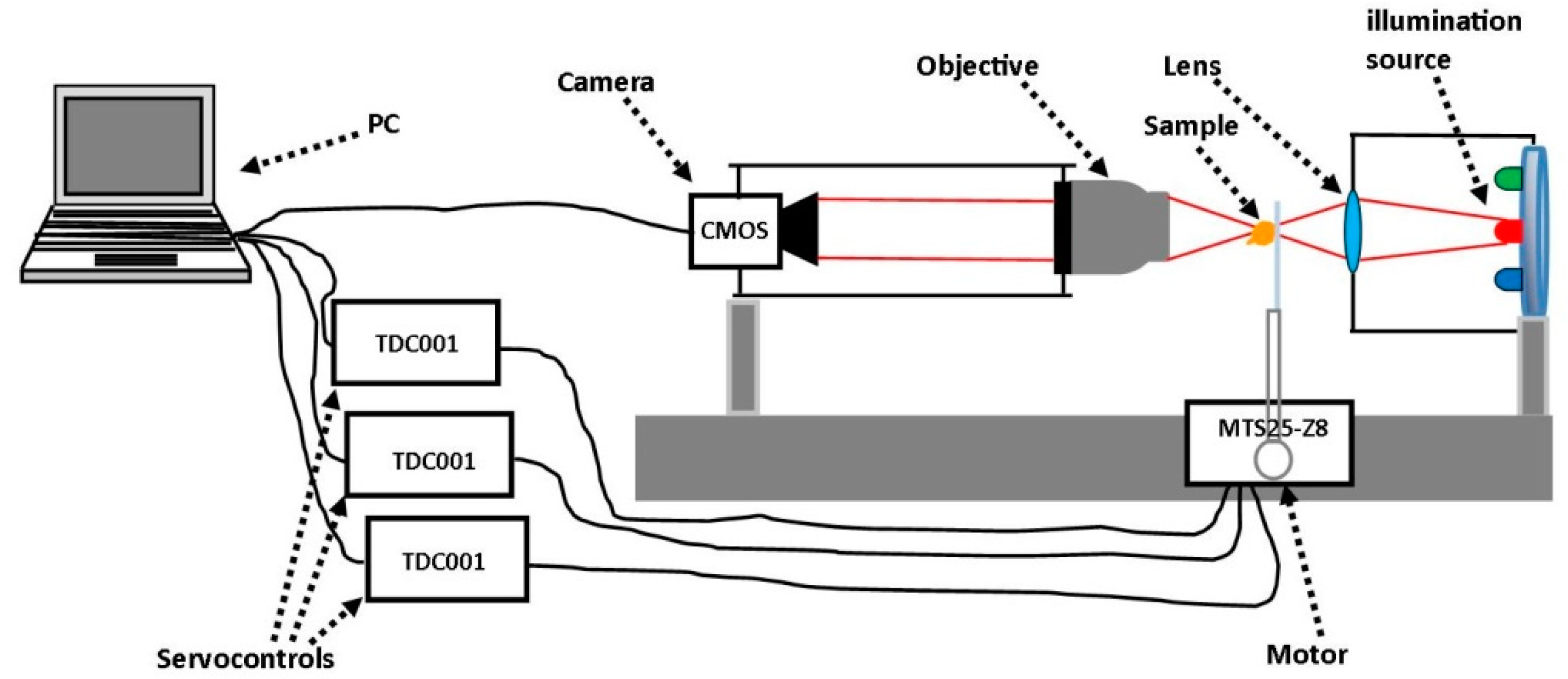
2.1. Experimental Set-Up

In Figure 1, we can see the set-up of the experimental device. This consisted of a BF horizontal microscope with a 16 bit monochrome Complementary Metal-Oxide-Semiconductor (CMOS) camera with a pixel size of 5.5 µm × 5.5 µm, and an effective image chip size of 11.264 mm × 5.984 mm, presenting 2048 × 1088 pixels. The microscope enabled automated sequential acquisition of the BF images. The images were recorded by defocusing the sample slightly in the z-direction (optical axis) through a stepper motor MTS25-Z8. The motor was monitored in three directions (X, Y, Z) by three servocontrols. Therefore, we were able to scan the region of interest in the sample. The servocontrols were connected to the PC, which enables the control of the defocus distance Δz and the image acquisition protocol by using a MatLab operation code.

2.2. Sample Preparation

In this work, the sample was made up of 1 µm polystyrene microspheres beads (refractive index n = 1.586 at wavelength λ   =   640   nm [9]) at the temperature T = 17 °C. The solution of microspheres was diluted with distilled water ( n = 1.33 at the temperature T = 17 °C). A small drop of the diluted solution was placed and spread on a slide made of the highest purity corrosion-resistant glass with dimensions 75 mm × 25 mm × 1 mm. After drying the sample for 30 minutes, it was used for microscopic examination under partially coherent illumination at a wavelength λ   =   640   nm .

2.3. Measurement Procedure

We performed the measurements in transmission mode. Three sets of images were recorded in the same conditions:
-
image Td, the contribution of the background and the dark current in the detector; it was achieved with nothing in the microscope and with the source illumination turned off;
-
image Tb, the bright reference; it was achieved with an empty slide in the microscope;
-
image Ts, the raw image of the sample, it was achieved with the sample in the microscope.
Each set of images was recorded for each plane of the sample by moving it along the optical axis. The corrected image T of the sample is defined by Equation (1) (flat-field correction), as is commonly described by Tadrous [10], Brydegaard et al. [11], and Agnero et al. [12]:
T = T s T d T b T d
This operation cancels out the different emissive yields of the light emitting diode (LED) source, electronic gains, and exposures for each illumination, and also the variation in the illumination intensity over the field of view [11].
In practice, one major disadvantage of TIE method is the sequential capture of images. It requires the precise motion of the sample, which can be shifted from a plane to another due to a little vibration in the measurement environment. This induces artefacts in some of the recorded images [13]. Therefore, care was taken to avoid any movement that was able to produce vibration as the image acquisition was running.

2.4. Analysis Methods

Optical systems generally are not free of aberrations or imperfections that affect the quality of the recorded images. Consequently, the image of a point object is an extended distribution of intensity called point spread function (PSF). During data analysis, we firstly sought to remove from the corrected images the distortions of observation due to the optical acquisition system and the contributions from out-of-focus planes for the sample. In this approach, we introduced the model of an appropriate PSF required for a deconvolution, which should remove any artefact. At the second time, we used the TIE method to extract the refractive index and the size of the specimen.
Deconvolution requires a realistic model of the phenomena that induce distortions in the image formation process. The term “deconvolution microscopy” generally assumes fluorescence microscopy [14,15], and PSF deconvolution imaging theory has traditionally been linked to fluorescence. A main reason behind this association is that for the case of self-luminous objects, one needs only to consider signal intensity, leading to a unique PSF and making deconvolution a linear process. In general, this is not the case in BF microscopy, where two point spread functions are needed to describe image formation [16]. In fluorescence microscopy, the 3D image i ( x ,   y ,   z ) of an object corresponds to the convolution of the object o ( x ,   y ,   z )   with the PSF(x, y, z) [17]:
i = o P S F + B
where B models noise, and the symbol ⊗ denotes the convolution operation. BF microscopy is presented as an alternative to fluorescence in deconvolution image processing, because of the possibility for observing unstained objects. However, its corresponding PSF consists of two separate components, one for phase ( P S F p ) and one for absorption ( P S F a ). Therefore, the BF-3D image i ( x ,   y ,   z ) is generally described as the sum of the convolutions of the real (P) and imaginary (A) parts of the object scattering potential with the corresponding PSFs [18]:
i = P P S F p + A P S F a + B
This excludes the application of linear deconvolution processing to remove distortion. However, in the presence of the pure phase object as it is the case in this work, BF imaging essentially reduces to Equation (2), making it possible to perform linear deconvolution [16]. Therefore, knowing the PSF leads to the determination of the object through deconvolution. The PSF can be:
-
computed from the optical properties of the microscope system,
-
estimated from the measurements of the microspheres.
The experimental PSF takes into account all of the aberrations introduced by the whole image acquisition system [19]. It is determined by recording images of a specimen (assumed to be a point object) in different planes of defocus above and below the focal plane. A point object does not exist in practical applications; the object necessarily has a particular size. Therefore, for the measured data to correspond to the microscope’s PSF, it is very important that the object size is smaller than the diffraction limit. If this is not the case, the measured data will instead correspond to the convolution of the PSF with the object shape, according to Equation (2) [20]. Unfortunately, using a very small object introduces the problem of signal detection, due to a very low signal-to-noise ratio. This requires detectors of high sensitivity. The signal to noise ratio is so low that often a bead is used whose size is not smaller than diffraction limit, but of the order of the microscope’s resolution [21]. This leads to an overestimated PSF. The experimental PSF is noisy and needs to be devoid of noise, which is a limitation in a deconvolution algorithm. The method of denoising sometimes distorts the real PSF of the microscope. Lai et al. [22] used a denoising method based on singular value decomposition to get a denoised PSF, but it produced small visible artificial ripples to the denoised PSF [19].
The computed PSF, in particular the model of Gibson and Lanni [23], also takes into account the conditions in which the experiment is carried out, and it has an advantage of being estimated for all of the object space. It is free of noise, flexible, and suitable to any specific condition of the experimentation, unlike experimental PSF, which is not modifiable because it is measured to represent a specific condition in which the images of biological sample must be recorded. The BF-PSF model was reported previously by Hernandez and Gutierrez [16]. However, they do not assume a real point object in their model. The model of Gibson and Lanni [23] is more an accurate model for PSF generation that is suitable for the brightfield setting [10], and this was discussed and publicly made available as an ImageJ plug-in by Besson et al. [24]. According to the model, the image of a point object located at X p = ( x p ,   y p ,   z p ) is defined by Equation (4) [23]:
P S F ( X , X p ) = | A 0 1 e i   w ( ρ ,   X ,   X p )   J 0 ( 2 π λ   r   N A   ρ ) ρ   d ρ | 2  
where X = ( x ,   y ,   z ) is a point on the image plane, N A is the numeric aperture of the objective, A is an amplitude constant, ρ is the radius of the microscope’s limiting aperture in the microscope’s back focal plane, J 0 denotes the Bessel function of the first kind of order zero, and w ( ρ ,   X ,   X p ) is the phase which enables aberrations to be taken into account in the model, r = ( x x p ) 2 + ( y y p ) 2 . The phase w ( ρ ,   X ,   X p ) is defined by Equation (5), as there are two layers (immersion medium of refractive index n c and the specimen layer of refractive index n m ) [25]:
w ( ρ ,   X ,   X p ) = k [ z p n m 2 N A 2 ρ 2 W D n c 2 N A 2 ρ 2 + ( z p z n + n c ( W D n c z p n m ) ) n c 2 N A 2 ρ 2 ]
The parameters n c and W D are the design refractive index of the immersion medium and working distance of the objective, respectively, and k is the wave number. The model of Gibson and Lanni [23] allowed for the restoration of our BF images.
Defining the wave field traversing the specimen by E z _ ( x , y ) = I z ( x , y ) e j ϕ z ( x , y ) , where I z ( x , y ) is the intensity, ϕ z ( x , y ) the phase, z denotes the position along the optical axis, and ( x , y ) are the two-dimensional coordinates in the plane orthogonal to the optical axis. Therefore, the denotation I z ( x , y ) indicates the intensity I ( x , y , z ) . The TIE is obtained by substituting E z _ ( x , y ) into the paraxial wave equation and taking the imaginary part of the resulting expression; the TIE is defined by [6]:
I z ( x , y ) z = λ 2 π · ( I z ( x , y ) ϕ z ( x , y ) )
where λ is the wavelength of the illumination source and denotes the gradient operator in the lateral dimensions ( x , y ) . Due to its non-interferometric nature, the illumination can be quasi-monochromatic and partially-coherent [26]. The numerical solution for the TIE in the case of a pure phase object (transparent object), is defined by Equation (7) [7], resulting from the standard equation of Poisson [27,28]:
ϕ z ( x , y ) = T F 1 [ T F [ 2 π λ   1 I z ( x , y )   I z ( x , y ) z ] 4 π 2 ( u 2 + ν 2 ) ]
where T F 1 and T F denote the inverse Fourier Transform and Fourier Transform respectively, and ( u , ν ) denotes the spatial frequency variables corresponding to the coordinates ( x , y ). Equation (7) is valid only for paraxial ray assumptions. The phase of the wave field is related to the variation of the image intensity along the optical axis through Equation (7). In practice, the intensity derivative I z ( x , y ) / z in the observation plane z cannot be measured directly; we adopted the following approximation (Equation (8)) using two defocused images, one above the observation plane ( I ( x , y , z + Δ z ) ) and one below ( I ( x , y , z Δ z ) ):
I z ( x , y ) z I ( x , y , z + Δ z ) I ( x , y , z Δ z ) 2 · Δ z
where Δ z is the defocus distance. Phase distortions induced in the wave field as the wave propagates from point r z 0 ( x , y ) to r z ( x , y ) can be related to the refractive index of the specimen through solutions to the eikonal equation [8,29] for the phase:
ϕ z ( x , y ) ϕ z 0 ( x , y ) = 2 π λ z 0 z Δ n z ( x ,   y ) d z
Δ n z ( x ,   y ) is the refractive index difference between the specimen and its surrounding medium (specimen layer). Taking the specimen to be located directly above the origin r z 0 ( x , y ) , hence ϕ z 0 ( x , y ) = 0 , and for points inside the specimen, it is found that [8]:
ϕ z ( x , y ) = 2 π λ 0 z Δ n z ( x ,   y ) d z
Therefore, if ϕ z ( x , y ) is known in multiples planes (with small value of defocus distance Δ z ) inside the specimen, its 3D refractive index distribution can be recovered via Equation (11) [30] through sequential method (using finite differences) applied to pairs of consecutive planes (one pair after one sequentially) with the same value of defocus distance:
n z ( x , y ) = n m + λ 2 π   ϕ z ( x , y ) z
where n m is the refractive index of the specimen layer. To retrieve the 2D phase ϕ z ( x , y ) corresponding to the observation plane z , we used Equation (7) and three recorded images of the sample were needed, one in the observation plane, and the both of the others below and above the observation plane with a defocus distance Δ z . This procedure was repeated to obtain ϕ z ( x , y ) in multiples planes by changing the observation plane with the same value of Δ z until the whole specimen was scanned along the optical axis. The defocus distance is an important factor in the quality of the reconstruction. When Δ z was large, the hypothesis of linearity that enables the above approximation (Equation (8)) of the intensity derivative I z ( x , y ) / z was not valid, and this nonlinearity affected the accuracy of the reconstruction. For small values of Δ z where the linearity was preserved, there was a reduction of signal to noise ratio due to the term I ( x , y , z + Δ z ) I ( x , y , z Δ z ) , which becomes smaller. This required a compromise between the defocusing, accuracy, and signal to noise ratio. Therefore, when we are in the presence of multiple plane images and we would like to retrieve the 2D phase ϕ ( x , y ) corresponding to the focal plane, we cannot simply use pairs of plane images to recover the phase from average of them [13]. In this work, we used the method proposed by Zhong et al. [31], which performs fitting (through Gaussian process regression) on each pixel’s intensity in the frequency domain along the optical axis, taking into account all the images in different planes. This method allowed an estimation of the derivative I z ( x , y ) / z , which led us to retrieve the phase in the focal plane. Consequently, the specimen’s size t ( x , y ) was obtained by using Equation (12) [32]:
t ( x , y ) = λ   ϕ ( x , y ) 2 π   ( n f n m )
where n f is the refractive index of the specimen in the focal plane.

3. Results and Discussion

During the computation of the PSF for our experimental device, two parameters were not directly accessible: the depth z p of the point object in the specimen layer, and the refractive index n c of the immersion medium (air) during the experimentation [25]. Our sample of microspheres of diameter 1 µm was allowed to dry during experimentation. This enabled us to assume that the point object was on the interface of air and specimen layer, so z p = 0. The measured pressure and temperature in the measurement environment ( P = 992   hPa , T = 17 °C) enabled the determination of the refractive index, n c , of the immersion medium (air) during experimentation; n c = 1.00024 by using Equation (13) [33,34]:
n c = 1 + ( 6.4328 · 10 5 + 2.94981 · 10 2 146 λ 2 + 2.554 · 10 4 41 λ 2 ) 15 · P T
where P , T , and λ are in bar, in degrees Celsius and in μ m respectively. Figure 2 presents the PSF of our device. The images of the sample in different planes were affected by the contribution of out-of-focus planes (Figure 3a–c). Restoration of these images was achieved by using the Richardson–Lucy algorithm [35,36] implemented in MatLab, taking into account the 3D-PSF. The number of iterations used was 25. This led to a reduction not only in the effects of diffraction but also in the noise and pixel intensity, due to the contribution of the adjacent planes (Figure 3d–f).
Applying the TIE method sequentially on the corrected images led to an extracted refractive index of the specimen (Figure 4a–g). We can observe in Figure 4a–g that the outlines of the microsphere became smaller as we moved away from the focal plane ( z = 0   μ m ). This was due to effect of sectioning. In a plane of the microsphere, the spatial distribution of its refractive index was not homogeneous. The homogeneity of refractive index distribution was drastically damaged as we moved away from the focal plane. This was due to diffraction effects [37] that became prominent. In this case, the paraxial ray assumptions, which were required to apply TIE, were nullified [8]. This induced artefacts in the refractive index reconstruction (Figure 4a–c). TIE method drastically failed to recover the 3D refractive index distribution of the sample for an optical system with a high numeric aperture, as was the case for our device ( N A o b = 0.75 ) [37].
A reconstruction of the refractive index after the deconvolution of the corrected images by the use of the 3D-PSF is presented in Figure 4h–n. The sectioning effect was more greatly appreciated through the spatial distribution of refractive index. The circular outlines of the microsphere were well highlighted. The artefacts that were observed in the planes z = 0.4   μ m , z = 0.3   μ m , z = 0.2   μ m were removed. In each plane of the microsphere, the homogeneity of refractive index distribution was greatly improved and tended to cover all of the circular outline of the microsphere, mostly in the focal plane. Table 1 presented a comparison between the mean values of the microsphere’s refractive index in the presence of the diffraction, and in the absence of diffraction. A mean value of the refractive index for the microsphere was an average over all the points inside the microsphere that corresponded to a plane. Before the deconvolution (presence of diffraction), the mean value of the refractive index seemed to be a function of the z-position. We mainly observed a decrease of refractive index values while we moved away from the focal plane. This was due to the diffraction dependence along the optical axis, which becomes more significant as we moved away from the focal plane. From z = 0.1   μ m to z = 0.2   μ m , an increase occurred. This could explain an effect of the vibration which occurred during the measurement. This induced the sample to be shifted from a plane to another during the measurement. This was a drawback for the TIE method, which required the precise motion of the sample. After the deconvolution (taking into account 3D-PSF), the mean value of the refractive index was quasi-constant. The value in the focal plane where diffraction effects are greatly reduced was also in agreement with the refractive index of 1.586 , which is the reference value [9] at 640   nm . In Figure 5, we can see the size’s map t ( x , y ) of the specimen. It was obtained by using Equation (12), taking n f = 1.587 as the mean value of microsphere’s refractive index in the focal plane and n m = 1.33 as the refractive index of the distilled water used in the sample preparation. The microsphere’s diameter as deduced from the map was d = 0.943   μ m . This value represents the intensity of the pixel in the middle of the microsphere (Figure 5). The graph for the mean values of the refractive index as a function of z-position also led to the recovery of the diameter of the microsphere. The diameter was defined by the full width at half maximum (FWHM) indicated in the graph by the double arrow (Figure 6). The diameter, which was deduced from the graph, is 1.1   μ m . These two diameter values were close to 1   μ m (the reference diameter of the microsphere used for the microscopic examination in this work), and they were in relative variation, between 6 % and 10 % .

4. Conclusions

In this work, we introduced a method to reconstruct the 3D refractive index distribution by combining TIE and deconvolution. A BF microscope using a camera was constructed, and the proposed technique was applied for a technical sample with well-known properties. The microscope’s 3D-PSF, which takes into account optical aberrations, was computed. Its influence on the 3D refractive index recovery, using the TIE method, was demonstrated. Experimental results show that taking the diffraction into account while performing TIE on BF-images can significantly improve the accuracy of the 3D refractive index reconstruction. It was demonstrated that the method is able to infer the size of the sample accurately. Therefore, this approach was used in our laboratory to extract the optical parameters. The proposed technique can be applied, not only to homogeneous specimens, but also to specimens presenting heterogeneous compositions in their structures, such as biological cells. However, they must be pure phase objects, where it is possible to perform linear deconvolution according to Equation (2); otherwise the proposed method cannot be used.

Author Contributions

M.A.A., K.K., and J.T.Z. conceived the technique presented in this work, and wrote the manuscript. A.T.K. and O.K.B. participated in the imaging acquisitions set-up for the experiment. The authors have all read and approved the submitted version of the manuscript.

Funding

This work was financially supported by the International Science Programme (ISP) and The World Academy of Sciences (TWAS).

Conflicts of Interest

The authors declare no conflict of interest.

References

  1. Barer, R.; Joseph, S. Refractometry of Living Cells Part I. Basic Principles. Q. J. Microsc. Sci. 1954, 95, 399–423. [Google Scholar]
  2. Zhuo, W.; Krishnara, T.; Balla, A.; Popescu, G. Tissue refractive index as marker of disease. J. Biomed. Opt. 2011, 16, 116017. [Google Scholar]
  3. YongKeun, P.; Monica, D.S.; Popescu, G.; Lykotrafitis, G.; Wonshik, C.; Feld, S.M.; Subra, S. Refractive index maps and membrane dynamics of human red blood cells parasitized by Plasmodium falciparum. Proc. Natl. Acad. Sci. USA 2008, 105, 13730–13735. [Google Scholar] [Green Version]
  4. Florian, C.; Anca, M.; Frédéric, M.; Jonas, K.; Tristan, C.; Etienne, C.; Pierre, M.; Christian, D. Cell refractive index tomography by digital holographic microscopy. Opt. Lett. 2006, 31, 178–180. [Google Scholar]
  5. Chao, Z.; Qian, C.; Anand, A. Transport of intensity equation: A new approach to phase and light field. Proc. SPIE 2014, 9271, 92710H. [Google Scholar]
  6. Teague, M.R. Deterministic phase retrieval: A Green’s function solution. J. Opt. Soc. Am. 1983, 73, 1434–1441. [Google Scholar] [CrossRef]
  7. Laura, W.; Lei, T.; Barbastathis, G. Transport of Intensity phase-amplitude imaging with higher order intensity derivatives. Opt. Express 2010, 18, 12552–12561. [Google Scholar]
  8. Kevin, G.P.; Steven, L.J.; Owen, J.T.M. Measurement of Single Cell Refractive Index, Dry Mass, Volume, and Density Using a Transillumination Microscope. Phys. Rev. Lett. 2012, 109, 118105. [Google Scholar]
  9. Ivan, D.N.; Christo, D.I. Optical plastic refractive measurements in the visible and the near-infrared regions. Appl. Opt. 2000, 39, 2067–2070. [Google Scholar]
  10. Tadrous, P.J. A method of PSF generation for 3D brightfield deconvolution. J. Microsc. 2009, 237, 192–199. [Google Scholar] [CrossRef] [PubMed]
  11. Brydegaard, M.; Merdasa, A.; Jayaweera, H.; Ålebring, J.; Svanberg, S. Versatile multispectral microscope based on light emitting diodes. Rev. Sci. Instrum. 2011, 82, 123106. [Google Scholar] [CrossRef] [PubMed] [Green Version]
  12. Agnero, M.A.; Zoueu, J.T.; Konan, K. Characterization of a Multimodal and Multispectral Led Imager: Application to Organic Polymer’s Microspheres with Diameter Φ=10.2μm. Opt. Photonics J. 2016, 6, 171–183. [Google Scholar] [CrossRef]
  13. Laura, W. Computational Phase Imaging Based on Intensity Transport. Ph.D. Thesis, Massachusetts Institute of Technology, Cambridge, MA, USA, 2010. [Google Scholar]
  14. McNally, J.G.; Karpova, T.; Cooper, J.; Conchello, J.A. Three-dimensional imaging by deconvolution microscopy. Methods 1999, 19, 373–385. [Google Scholar] [CrossRef] [PubMed]
  15. Swedlow, J.R. Quantitative fluorescence microscopy and image deconvolution. Methods Cell Biol. 2007, 81, 447–465. [Google Scholar] [PubMed]
  16. Hernandez, C.N.; Gutierrez-Medina, B. Direct Imaging of Phase Objects Enables Conventional Deconvolution in Bright Field Light Microscopy. PLoS ONE 2014, 9, e89106. [Google Scholar] [CrossRef] [PubMed]
  17. Chrysanthe, P.; Michael, I.M.; Lewis, J.T.; James, G.M. Regularized linear method for reconstruction of three-dimensional microscopic objects from optical sections. J. Opt. Soc. Am. 1992, 9, 209–228. [Google Scholar]
  18. Streibl, N. Three-dimensional imaging by a microscope. J. Opt. Soc. Am. A 1985, 2, 121–127. [Google Scholar] [CrossRef]
  19. Laasmaa, M.; Vendelin, M.; Peterson, P. Application of regularized Richardson-Lucy algorithm for deconvolution of confocal microscopy images. J. Microsc. 2011, 243, 124–140. [Google Scholar] [CrossRef] [PubMed]
  20. Yasushi, H.; John, W.S.; Agard, D.A. Determination of three-dimensional imaging properties of a light microscope system Partial confocal behavior in epifluorescence microscopy. Biophys. Soc. 1990, 57, 325–333. [Google Scholar]
  21. Haeberlé, O.; Bcha, F.; Simler, C.; Dieterlen, A.; Xu, C.; Colicchio, B.; Jacquey, S.; Gramain, M.P. Identification of acquisition parameters from the point spread function of a fluorescence microscope. Opt. Commun. 2001, 196, 109–117. [Google Scholar] [CrossRef]
  22. Lai, X.; Lin, Z.; Ward, E.S.; Ober, R.J. Noise suppression of point spread functions and its influence on deconvolution of three-dimensional fluorescence microscopy image sets. J. Microsc. 2005, 217, 93–108. [Google Scholar] [CrossRef] [PubMed] [Green Version]
  23. Gibson, S.F.; Lanni, F. Experimental test of an analytical model of aberration in an oil-immersion objective lens used in three-dimensional light microscopy. J. Opt. Soc. Am. 1991, 8, 1601–1613. [Google Scholar] [CrossRef]
  24. Besson, P.; Vonesch, C.; Aguet, F. PSF Gibson generator plug-in for Image-J. v.1.0. 2005. Available online: http://bigwww.epfl.ch/demo/deconvolution3D/ (accessed on May 2009).
  25. Aguet, F.; Dimitri, D.V.; Unser, M. An accurate PSF model with few parameters for axially shift-variant déconvolution. In Proceedings of the 2008 5th IEEE International Symposium on Biomedical Imaging: From Nano to Macro, Paris, France, 14–17 May 2008; pp. 157–160. [Google Scholar]
  26. Chao, Z.; Qian, C.; Anand, A. Comparison of Digital Holography and Transport of Intensity for Quantitative Phase Contrast Imaging. In Fringe; Osten, W., Ed.; Springer: Berlin/Heidelberg, Germany, 2013. [Google Scholar] [CrossRef]
  27. Gureyev, T.; Nugent, K. Rapid quantitative phase imaging using the transport of intensity equation. Opt. Commun. 1997, 133, 339–346. [Google Scholar] [CrossRef]
  28. Allen, L.J.; Oxley, M.P. Phase retrieval from series of images obtained by defocus variation. Opt. Commun. 2001, 199, 65–75. [Google Scholar] [CrossRef]
  29. Ishimaru, A. Wave Propagation and Scattering in Random Media, Part II; Academic: New York, NY, USA, 1978; Chapter 7. [Google Scholar]
  30. Liu, P.Y.; Chin, L.K.; Ser, W.; Chen, H.F.; Hsieh, C.M.; Lee, C.H.; Sung, K.B.; Ayi, T.C.; Yap, P.H.; Liedberg, B.; et al. Cell refractive index for cell biology and disease diagnosis: past, present and future. R. Soc. Chem. 2016, 16, 634–644. [Google Scholar] [CrossRef] [PubMed]
  31. Zhong, J.; Claus, A.R.; Dauwels, J.; Lei, T.; Laura, W. Transport of Intensity phase imaging by intensity spectrum fitting of exponentially spaced defocus planes. Opt. Express 2014, 22, 10662–10674. [Google Scholar]
  32. Rodrigo, J.A.; Alieva, T. Rapid quantitative phase imaging for partially coherent light microscopy. Opt. Express 2014, 22, 13472–13483. [Google Scholar] [CrossRef] [PubMed]
  33. James, C.O. Optical Refractive Index of Air: Dependence on Pressure, Temperature and Composition. Appl. Opt. 1967, 6, 51–59. [Google Scholar]
  34. Garrel, V. Réalisation d’un instrument d’imagerie visible à la limite de diffraction pour un grand télescope. Ph.D. Thesis, École doctorale d’Astronomie et d’Astrophysique, Ile de France, Meudon, France, 2012; pp. 1–11. [Google Scholar]
  35. Richardson, W.H. Bayesian-Based Iterative Method of Image Restoration. J. Opt. Soc. Am. 1970, 62, 55–59. [Google Scholar] [CrossRef]
  36. Lucy, L.B. An iterative technique for the rectification of observed distributions. Astron. J. 1974, 79, 745–749. [Google Scholar] [CrossRef]
  37. Wonshik, C.; Fang-Yen, C.; Badizadegan, K.; Dasari, R.R.; Feld, M.S. Extended depth of focus in tomographic phase microscopy using a propagation algorithm. Opt. Lett. 2008, 33, 171–173. [Google Scholar]
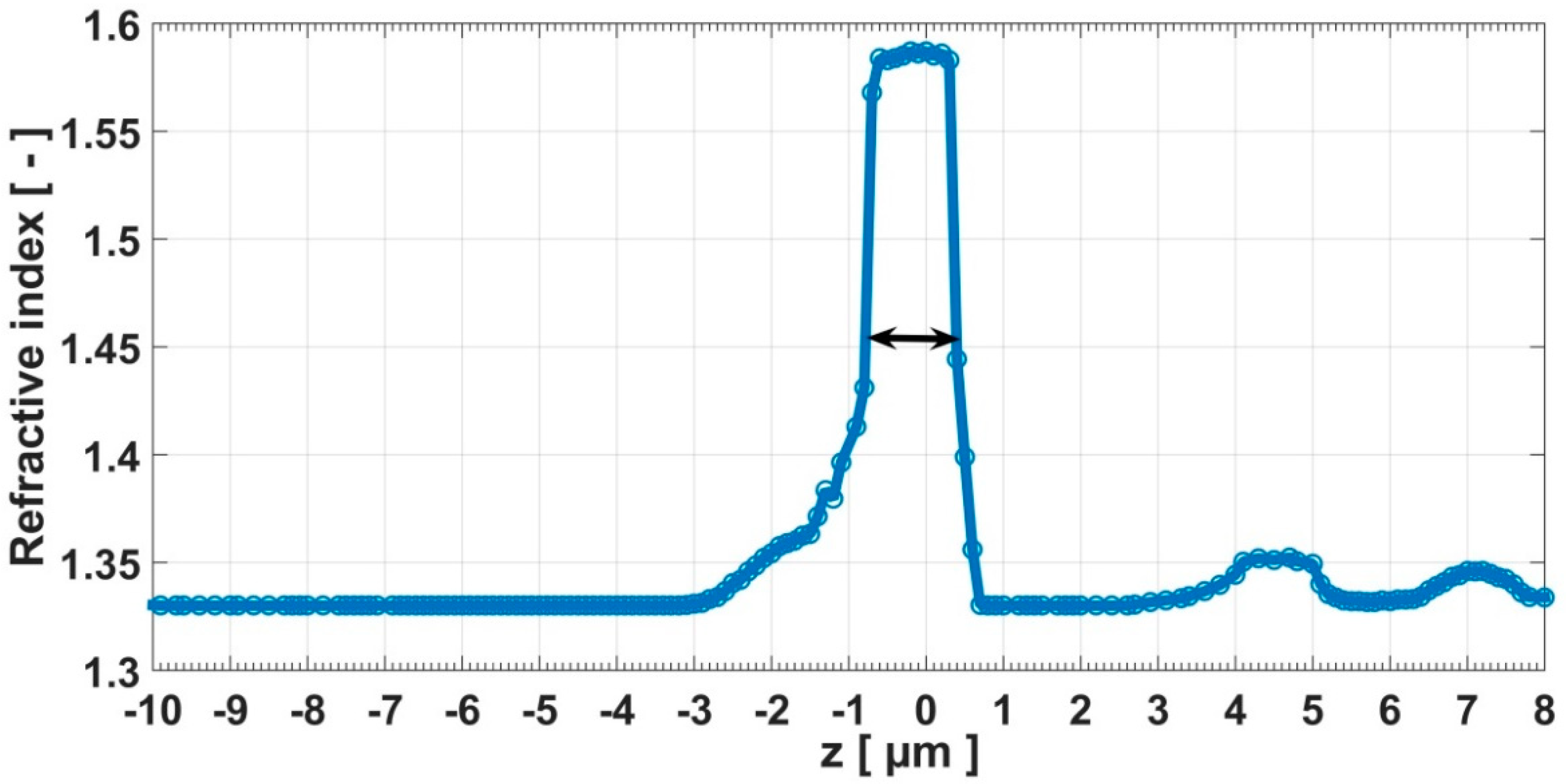
Figure 1. Set-up of the microscope constructed for automated image acquisition. The red lines illustrate the beam path interacting with the sample.
Applsci 08 01649 g001
Figure 2. X–Z cross section of the computed point spread function (PSF) with the acquisition parameters of the experimental device: the numeric aperture of the dry objective N A o b = 0.75 with working W D = 0.71   mm ; the refractive index of specimen layer n m = 1.33 ; the standard value of refractive index of the air n c = 1 ; the refractive index of the air during the experimentation n c = 1.00024 , z p = 0 ; the pixel size in the object space is 0.1 µm.
Applsci 08 01649 g002
Figure 3. Recorded images in the different planes of a polystyrene microsphere of diameter 1   μ m at the wavelength λ = 640   nm (ac), and the corresponding restored images (df).
Applsci 08 01649 g003
Figure 4. 3D refractive index reconstruction at 640   nm for a polystyrene microsphere with a diameter of 1   μ m , without PSF consideration (ag), and with PSF consideration (hn).
Applsci 08 01649 g004
Figure 5. Size’s map for the sample. The intensity of each pixel at a point of the microsphere indicates in μm the thickness (at this point) of the microsphere. The intensity of the pixel in the middle of the microsphere represents its diameter, as indicated by the arrow.
Applsci 08 01649 g005
Figure 6. Mean values of the refractive index of the microsphere as a function of the z-position along the optical axis. The full width at half maximum (FWHM) indicated by the double arrow corresponds to the diameter of the microsphere.
Applsci 08 01649 g006
Table 1. Mean values of the refractive index of the microsphere at the wavelength 640 nm for each plane Z (μm).
Z = −0.4Z = −0.3Z = −0.2Z = −0.1Z = 0Z = 0.1Z = 0.2
Refractive index before deconvolution1.4441.4601.5261.5121.5561.5581.515
Refractive index after deconvolution1.5841.5851.5871.5861.5871.5851.586

