Article

Event-Driven Sensor Deployment in an Underwater Environment Using a Distributed Hybrid Fish Swarm Optimization Algorithm

1
Department of Electrical Engineering and Computer Science, Ningbo University, Ningbo 315211, China
2
Department of Computer Science Engineering, Ningde Normal University, Ningde 352000, China
*
Author to whom correspondence should be addressed.
Appl. Sci. 2018, 8(9), 1638; https://doi.org/10.3390/app8091638
Submission received: 4 August 2018 / Revised: 6 September 2018 / Accepted: 10 September 2018 / Published: 13 September 2018
(This article belongs to the Special Issue Swarm Robotics)

Abstract

:
In open and complex underwater environments, targets to be monitored are highly dynamic and exhibit great uncertainty. To optimize monitoring target coverage, the development of a method for adjusting sensor positions based on environments and targets is of crucial importance. In this paper, we propose a distributed hybrid fish swarm optimization algorithm (DHFSOA) based on the influence of water flow and the operation of an artificial fish swarm system to improve the coverage efficacy of the event set and to avoid blind movements of sensor nodes. First, by simulating the behavior of foraging fish, sensor nodes autonomously tend to cover events, with congestion control being used to match node distribution density to event distribution density. Second, the construction of an information pool is used to achieve information-sharing between nodes within the network connection range, to increase the nodes’ field of vision, and to enhance their global search abilities. Finally, we conduct extensive simulation experiments to evaluate network performance in different deployment environments. The results show that the proposed DHFSOA performs well in terms of coverage efficacy, energy efficiency, and convergence rate of the event set.

1. Introduction

Underwater acoustic sensor networks (UASNs) are new network systems developed for underwater monitoring. UASNs are composed of numerous sensor nodes with capabilities that include information perception, data storage, data processing, underwater acoustic communication, and more. UASNs have been drawing increasing attention from both governments and research centers due to their extensive use in marine resources surveys, pollution monitoring, aided-navigation, and tactical surveillance. They are a hot topic in the study of sensor networks [1,2].
Recent studies of UASNs have mainly focused on node deployment, location tracking, routing algorithms, energy efficiency strategies, water safety, and other practical aspects. However, the research on node deployment of UASNs (also called coverage control) actually has its shortcomings [3,4,5]. Node deployment in UASNs has unique challenges which are not found in the deployment of land sensor networks. These include the influence of ocean currents and other factors, the fact that the underwater environments and monitoring targets are more dynamic than their land counterparts, and the challenge that underwater sensor nodes cannot be static and fixed in the monitoring space; instead, network topology must evolve gradually with network operation [6,7,8]. Therefore, developing a method for adjusting the position of sensor nodes autonomously in response to a changing environment, as well as achieving an effective monitoring system for target waters, are two of the problems researchers face when employing underwater wireless sensor networks.
In recent years, UASN deployment algorithms have mainly included graph-based classes [9], body-centered cubes [10], virtual force classes [11], and group-based intelligent optimization classes [12]. The first three types of redeployment algorithms are relatively complex and thus are not suitable for solving large-scale underwater environment problems. The group-based intelligence optimization algorithm [13], however, can generally determine the optimal solution of a complex optimization problem faster than traditional optimization algorithms [14]. This algorithm is simple to calculate, is neither a centralized nor a global model, and is highly versatile since it utilizes the advantages of group distributed searching. The artificial fish swarm algorithm is an emerging metaheuristic, bionic cluster, intelligent optimization algorithm. Inspired by the operation of the fish swarm system, this paper proposes a distributed hybrid fish swarm optimization algorithm (DHFSOA). The proposed DHFSOA is implemented and its performance is evaluated by simulation.
The following is the general framework of this paper: Section 2 introduces related works; Section 3 defines the underwater sensor deployment problem and its performance metrics; Section 4 presents a detailed introduction to the DHFSOA algorithm; Section 5 consists of a comprehensive evaluation; Section 6 contains our summary and conclusions.

2. Related Works

Swarm Intelligence (SI) is a feature of subjects without intelligence or with simple intelligence exhibiting intelligent behavior through any form of aggregation and collaboration. It is an important branch of artificial intelligence (AI) [15]. Without centralized control and without providing a global model, swarm intelligence provides the basis for finding solutions to complex distributed problems. At present, many research achievements have been made in the field of underwater sensor network coverage control. This section will summarize the coverage control algorithm based on group intelligence optimization.
Iyer [16] proposed an underwater sensor network positioning and deployment scheme based on the genetic algorithm of optimization technology, which determined the fewest number of nodes required to cover an area of interest (AOI). However, this kind of algorithm is obviously easy to fall into local optimum when the network connectivity is not high, and the influence of water flow is not considered. Yiyue [17] proposed an optimal deployment algorithm based on an artificial fish swarm algorithm. This deployment algorithm simulates the preying and following behaviors of artificial fish in order to determine the maximum coverage value. The proposed artificial fish deployment algorithm improves the coverage performance of the common artificial fish algorithm. The inadequacy is that it does not take into account the self-adaptability of the search step size and the information sharing of all nodes in the network, so it is easy to fall into local optimum in the later stage. Dhillon [18] proposed the max average coverage deployment (MACD) algorithm, which uses the grid model to simulate the monitoring area and completes node deployment by utilizing the greedy iterative strategy. The MACD can achieve higher network coverage and connectivity rates, even achieving full network coverage and connectivity. However, since high node density is needed for its successful deployment, this algorithm cannot be applied in situations with sparse underwater sensor network deployment.
In response to the aforementioned shortcomings, Du [19] proposed a particle swarm-inspired underwater sensor self-deployment (PSSD) algorithm that fully utilizes the behavioral characteristics of particle swarms and effectively solves the network coverage problem. However, there exist two obvious disadvantages in this algorithm, one is that it only considers the network coverage of events, and it is difficult to obtain higher network connectivity rates. In addition, since nodes may move blindly when using this algorithm, given their limited energy and the large energy consumption in an underwater environment, underwater nodes will die due to the rapid exhaustion of energy. The other is that the PSSD algorithm was inspired by the classic group intelligence optimization algorithm-particle swarm optimization (PSO). For the traditional optimization algorithm, PSSD is a simple and effective optimization problem, with one obvious drawback, which is the tendency to fall into local extremes [20].
Taking into consideration both the effectiveness and the limitations of the above PSSD algorithm, as well as the non-uniform deployment of underwater monitoring nodes, a distributed hybrid fish swarm optimization algorithm (DHFSOA) is proposed. The DHFSOA provides sensor nodes with an autonomous tendency to cover events by simulating fish foraging behavior and congestion control. Additionally, the concept of an “information pool” is introduced in order to expand the visual range of nodes and avoid blind movements, thus reducing node energy consumption during deployment.

3. Preliminaries

3.1. Description of the Problem

Assume that n underwater sensor nodes are deployed in the monitoring area A and s i represents the ith node in the network, so that the corresponding sensor node set is S = s 1 , s 2 , , s n . The dynamic point e, which users are interested in, is referred to as an event; thus, in monitoring area A, the event set E = e i e i A , i = 1 , 2 , , m . Assuming that any underwater node has the ability to sense, communicate, and move, B j = r j s , r j c , l j , P j , where r j s , r j c , l j , P j respectively represent the radius of perception, the radius of communication, the maximum moving step length of node s j , and the current position of the node s j , and r j s 0 , r j c 0 , and l j 0 0 j n . In a homogeneous network, all nodes have the same attributes, which are r j s = r s , r j c = r c , and l j = l 0 j n . A sensor node can sense an event and communicate with its neighbor nodes to obtain status information (number of events covered) of neighbor nodes. The task of a node is to cover an event, collect information about the event, and maintain connectivity between nodes.

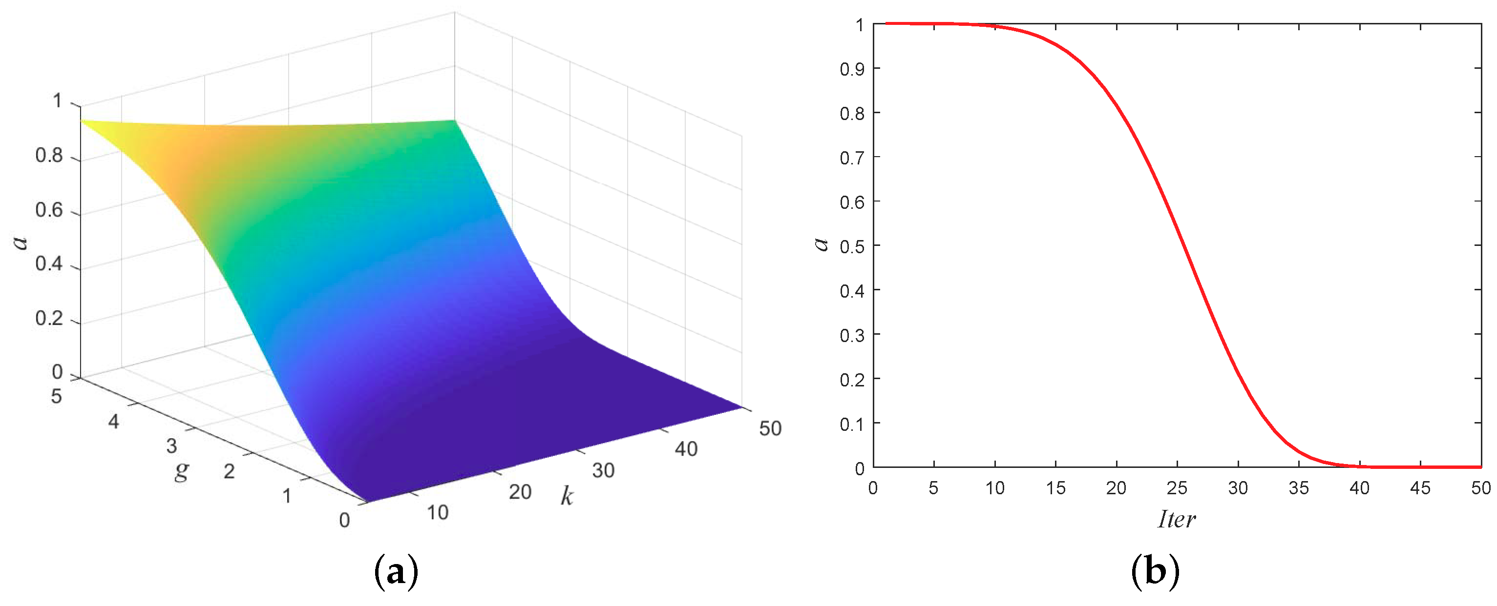
3.2. Coverage Perception Model

It is assumed that in the monitoring area A, the coverage model of each underwater sensor node is a sphere with the sphere’s center as the node’s coordinates and r j s as its radius of perception. The communication range is also a sphere, with radius r j c . To ensure the connectivity of the network, the radius of communication is set to be greater than or equal to twice the radius of perception; that is, r j c 2 r j s [21]. Assume the Euclidean distance d e i , s j between event e i and sensor node s j is
d e i , s j = x j x i 2 + y j y i 2 + z j z i 2 ,
where coordinate x j , y j , z j is the coordinate of node s j and coordinate x j , y j , z j is the coordinate of event e i . The probability that the defined event e i is covered by the sensor node s j is p e i , s j . A Boolean sensor coverage model is used to simplify the computation, and the probability is a binary function [22]:
p e i , s j = 1 , d e i , s j r s , 0 , o t h e r w i s e .
If d e i , s j r s , node s j covers event e i . In this case P e i , s j equals 1; otherwise, it is equal to 0. Similar to the calculation process for a two-dimensional sensor coverage area, the probability that the underwater three-dimensional space event e i is covered by node set S is P e i , S , where
p e i , S = p e i , s 1 p e i , s 2 p e i , s N = 1 i = 1 N 1 p e i , s i .
Definition 1.
According to the preceding analysis, the relative effective coverage degree of event e i can be described as [19]:
D A e i = s j S p e i , s j 1 + e i E I d e i , s j r s ,
where I ( · ) is an indicator function, that is, when the condition d e i , s j r s is satisfied, I d e i , s j r s is equal to 1; otherwise, it is 0. e i E I ( d ( e i , s j ) r s ) indicates the number of adjacent events e i for node s j .

3.3. Evaluation Standards

In this section, we introduce the coverage efficiency of the event set as well as the network coverage in order to measure the performance of the proposed method.
Definition 2.
Coverage entropy of the event set [19]. This measures the degree of coverage uniformity, and can be calculated as
H A E = e i E D A e i lg 1 D A e i ,
where the normalized coverage degree D A e i is
D A e i = D A e i e j E D A e j .
It is well known that the coverage entropy of event set H A E reaches its maximum value lg m only when D A e i = 1 m (for i = 1 , , m ) has equal probability.
Definition 3.
Network coverage C v is
C v = t e ˜ t e ,
where t e ˜ is the number of the events covered by nodes and t e is the total number of the events.
Definition 4.
The coverage efficiency of the event set is [19]
η E = α H A E lg m + β n ˜ n ,
where α , β [0, 1], α + β = 1 and n ˜ is the number of events covered by nodes.
From Definition 4, we can see that when all nodes cover events, that is, n = n ˜ , and simultaneously the coverage entropy H A E reaches a maximum value of lg m , η E will reach its maximum value of 1. Putting it simply, the main goal of underwater node deployment is to place nodes so as to achieve the maximum value of η E .

4. Node Deployment Scheme for UASNs Based on the DHFSOA
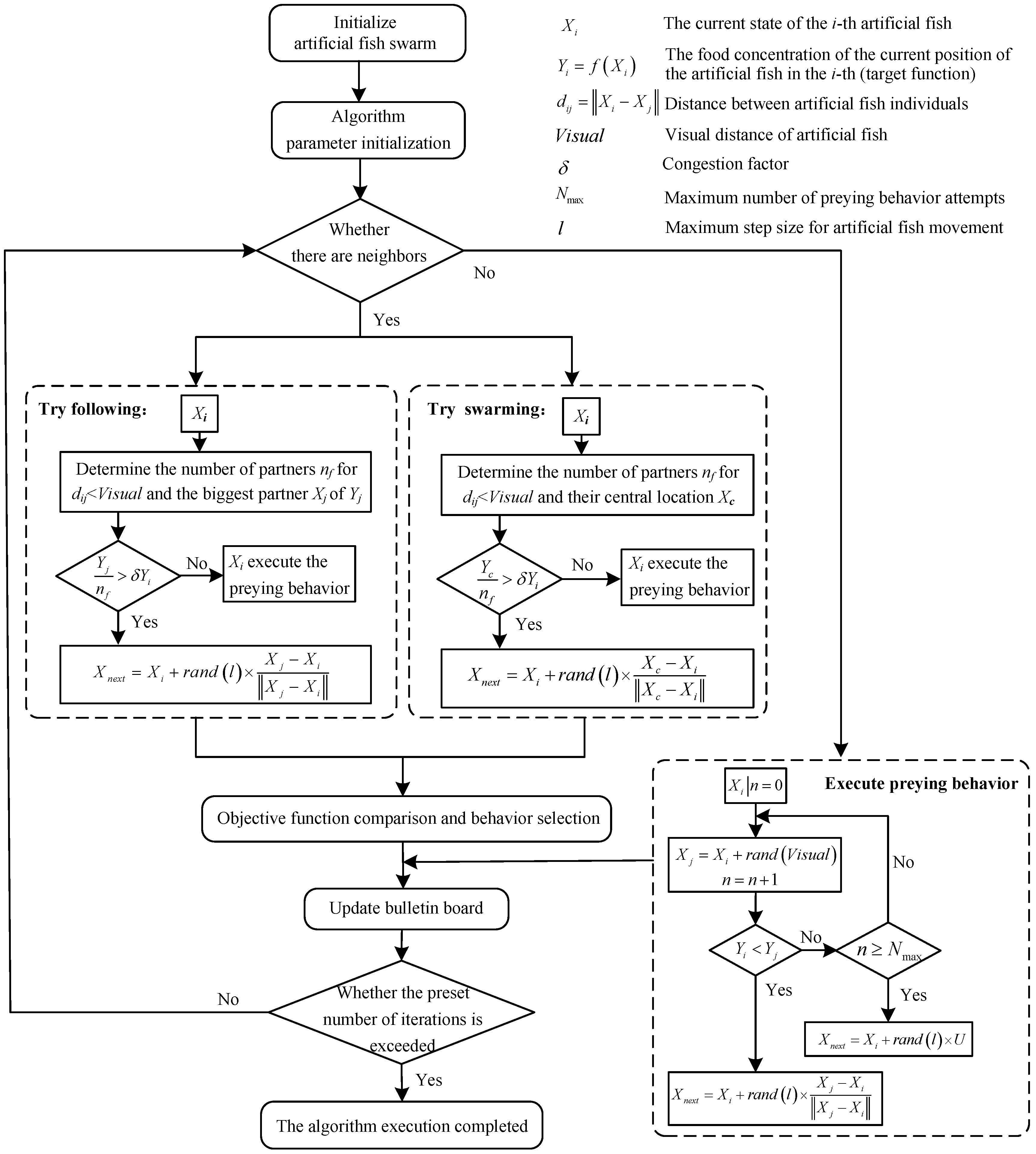
The artificial fish swarm algorithm (AFSA) is a heuristic intelligent search algorithm for global optimization. By simulating the preying and survival activities of fish, the AFSA can solve combination optimization problems such as optimal ordering, grouping, or screening of discrete events with a faster convergence speed than previous methods. The fish swarm algorithm and the underwater mobile sensor network are intrinsically related. The sensor node in the sensor network is equivalent to the artificial fish in the AFSA, events are equivalent to food, and the process of the node sensing the event is equivalent to the process of artificial fish searching for food. Therefore, the AFSA has been widely used in underwater mobile sensor networks.
In this study, we propose a DHFSOA and apply it to UASNs. Inspired by the operation of the fish swarm system, the DHFSOA gives the sensor nodes an autonomous tendency to cover events by simulating fish foraging and adjusts the distribution of nodes based on the degree of congestion. Additionally, the concept of an “information pool” is proposed, which expands the node’s visual range and accelerates the algorithm’s global search capability. Figure 1 is the flow chart of the artificial fish swarm algorithm. Behaviors such as preying, following, and swarming, which occur when fish forage, are the basis for the overall optimization.
(1)
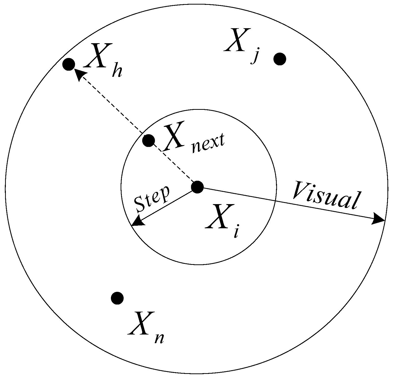
Preying behavior: preying behavior consists of fish randomly swimming in search of food; let the current state of the artificial fish be X i , randomly select a state X j within its visual range. When the maximal value problem is obtained, if Y i < Y j , then go further in the direction, that is X n e x t ; otherwise, re-randomly select the state X j , judging whether the forward condition is satisfied; after repeatedly trying N m a x times, if the forward condition is still not satisfied, the step is randomly moved.
(2)
Following behavior: following behavior occurs when a fish finds a location with abundant food and other fish quickly follow; suppose the current state of the artificial fish is X i , the number of partners in the current neighborhood ( d i j < V i s u a l ) is n f , and the partner with the highest food concentration among the ( n f ) partners is X j (food concentration is Y j ), if Y j n f > δ Y i , indicating that the state of partner X j has a higher food concentration and it is not too crowded around, then goes further in the direction of X j ; otherwise, the preying behavior is performed.
(3)
Swarming behavior: swarming behavior is the tendency for fish to naturally gather in groups while swimming. Set the number of partners in the current neighborhood ( d i j < V i s u a l ) to be n f , and the central position status to be X c . if Y c n f > δ Y i , indicating that the partner center has more food and the surrounding area is less crowded, moving further toward the partner center position X c ; otherwise, the preying behavior is performed.
Of course, the proposed DSFSOA mainly includes two kinds of behaviors: preying and following. In the following sections, the DHFSOA will be described in detail.

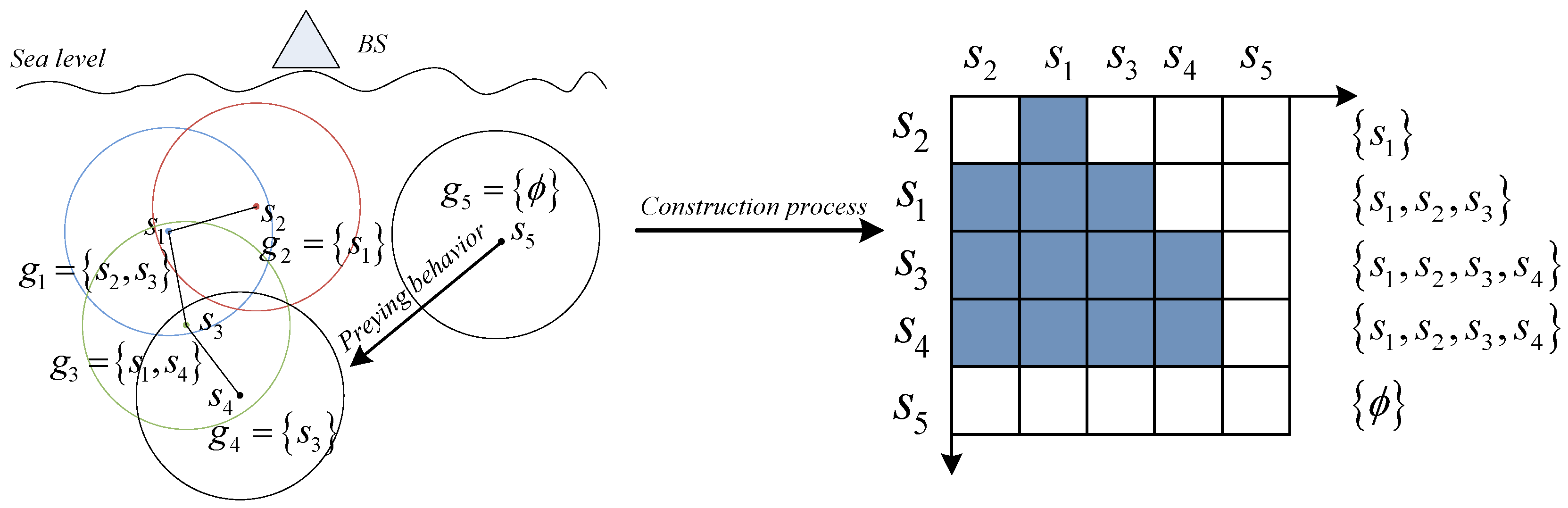
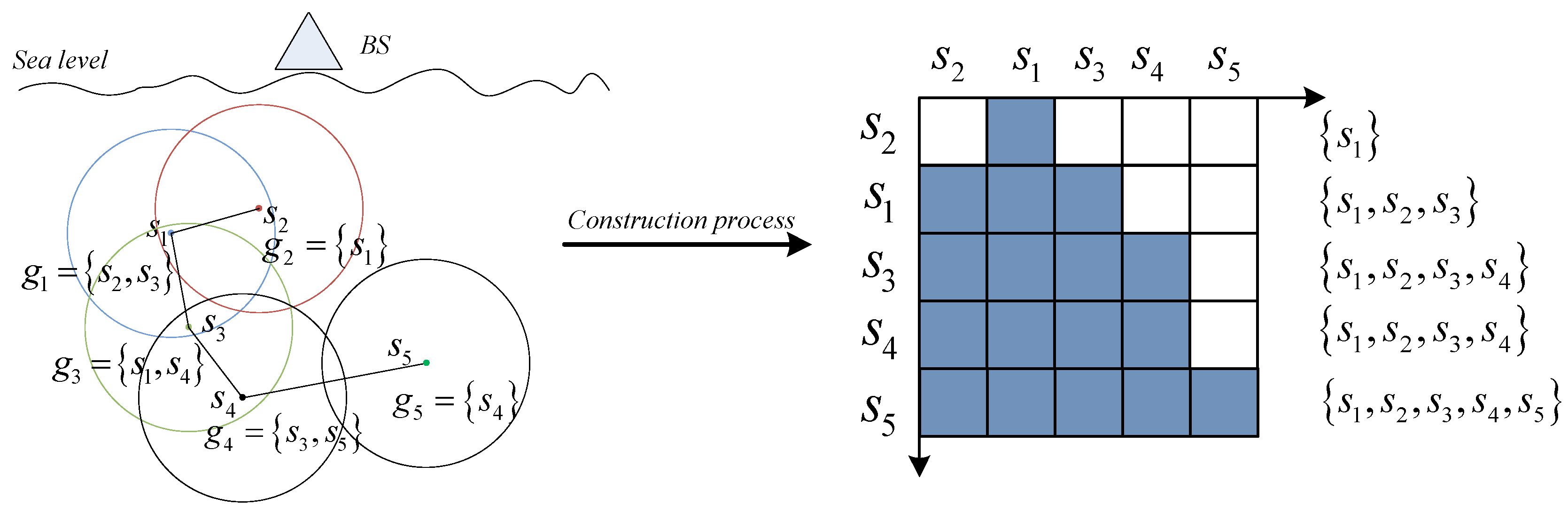
4.1. Construction of the Information Pool

Fish, whether real or artificial, rely on their vision to perceive external conditions, as shown in Figure 2. Here, X i is the current position of the artificial fish, V i s u a l is its visual range, and X h is the visual position at a particular time. If the concentration of food at the visual position is greater than that of the current position, it is assumed that the fish will proceed towards the visual position, thus arriving at the next position, X n e x t . Otherwise, the artificial fish continues to swim within its visual range. The more the fish swims within its visual range, the more comprehensive the understanding of the state within its visual range will become. This results in a full-scale, stereoscopic perception of the surrounding environment, which aids with corresponding judgments and decisions.
The sensor node in the DHFSOA is equivalent to the artificial fish in the AFSA, the radius of the communication r c is equivalent to the visual range of the artificial fish, and the event is equivalent to the food. The process of the mobile node exploring the larger network coverage in the sensor network is similar to the preying and following behaviors of individual artificial fish, and the network coverage of the sensor nodes is analogous to the food concentration in the environment of the artificial fish. However, the traditional artificial fish swarm algorithm cannot be directly applied to the underwater sensor network, mainly due to the fact that sensor nodes have limited amounts of energy. Given this limitation, excessive exploration by sensor nodes within their visual range will lead to their premature death. To enhance the global optimization and neighborhood search capabilities of the artificial fish swarm algorithm, while at the same time avoiding falling into a local optimum, an information pool is introduced here. As shown in Figure 3, it is assumed that there are five nodes in the underwater sensor network S = s 1 , , s 5 , and that each node can sense the surrounding events, here the event coverage is defined as the concentration F = f 1 , , f 5 . If all other nodes within the radius of communication of a node are referred to as neighbor nodes, then the neighbor nodes of the five nodes s i ( i = 1 , 2 , , 5 ) are represented as g 1 = s 2 , s 3 , g 2 = s 1 , g 3 = s 1 , s 4 , g 4 = s 3 , and g 5 = ϕ .
The information pool (which can also be thought of as a set) is constructed as follows: each node s i transmits data (the data mainly consist of the neighbor nodes and the number of coverage events) to each of its neighbor nodes through the network, and each neighbor node then transmits data to neighbor nodes other than the node that sent the data. Continue in this fashion until the data have traversed all the nodes in the connected state. Thus, the information pool in Figure 3 consists of node s 1 , s 2 , s 3 , and s 4 , that is, C s u m = s 1 , s 2 , s 3 , s 4 , and node s 5 is an isolated point. The benefits of the information pool in DSFSOA do not just include an increase in the global search speed of nodes (analogous to fish), but also consist of improvements in network connectivity through collaboration between nodes. As shown in Figure 4, the isolated node s 5 improves its isolated state through the preying behavior, establishes the connectivity between the node s 5 and the network, and expands the amount of information in the information pool, that is, C s u m = s 1 , s 2 , s 3 , s 4 , s 5 , The next step will be to focus on the self-organizing deployment process of nodes. The pseudo-code of the information pool construction algorithm is in Algorithm 1.
Algorithm 1: Construction of the Information Pool (Output Set C s u m ).
1:
s i a node in monitoring area A;
2:
Compute the set formed by node s j , neighbor of node s i , C i = { s j | d ( s i , s j ) r c } ;
3:
C s u m = C i { s i } ;
4:
C t m p = C i ;
5:
while C t m p 0 do
6:
   C k = j = 1 C t m p s k d s k , s j r c ;  
7:
   C t m p = C k C s u m ;
8:
   C s u m = C k C s u m ;
9:
end while
10:
Output C s u m ;

4.2. Description of Artificial Fish Behaviors

The artificial fish swarm optimization algorithm is a centralized, group intelligence search method. Inspired by the operation of the artificial fish swarm system, this paper proposes a distributed and achievable underwater sensor node deployment algorithm, the DHFSOA. The process in which nodes in the sensor network tend to increase network coverage is similar to the preying and following behaviors of artificial fish. Prior to introducing the two behaviors, the following definitions are provided:
Definition 5.
Congestion. The allowed congestion of node s i in monitoring area A is
σ s i = ψ · N e s i ,
where the constant ψ represents the expected coverage of a single event and N e s i represents the number of events covered by node s i , expressed as
N e s i = e j E p e j , s i .
Definition 6.
The number of nodes N n e s s i within the communication range and the number of nodes N c o s s i within the perceived range of the node s i can be expressed as
N n e s ( s i ) = c a r d ( λ ( s j ) ) ,
where c a r d ( λ ( s j ) ) indicates the number of nodes in the collection λ ( s j ) , λ s j = s j d s i , s j r c , 1 i , j n , i j represents the set of nodes s j within the communication radius of the node s i , and d s i , s j represents the Euclidean distance between node s i and s j :
N c o s ( s i ) = c a r d ( γ ( s j ) ) ,
where γ s j = s j d s i , s j r s , 1 i , j n , i j represents the set of nodes s j within the perceived range of the node s i
Next, the behavioral description of the artificial fish will be specifically described. n sensor nodes are randomly scattered in the underwater monitoring area A. Node s i may perform the following operations based on its own status as well as that of its neighbor nodes:
(1)
Following behavior: Set the number of partners in the visible domain (radius of communication being r c ) of node s i as N n e s s i , N n e s s i > 0 and information pool built with the partners as C s u m , and determine the optimal node s o p t in C s u m ,
s o p t = arg max s k C s u m N n e s s k .
If node s i finds more events covered at s o p t and s o p t is less crowded, i.e., N e s o p t N e s i and N c o s s o p t < σ s o p t , then move one step toward the position of partner s o p t :
X n e x t = X i + r a n d l × X o p t X i X o p t X i ,
where X i and X o p t represent position vectors of s i and s o p t respectively, and l is the value of the moving step.
(2)
Preying behavior: Set the number of partners in the visible domain (radius of communication being r c ) of node s i as N n e s s i , N n e s s i = 0 , which indicates that node s i is in an isolated state. l is the maximum value of the moving step. Set the current position of node s i as x i , and randomly move to the new position x j within its maximum moving step l:
X n e x t = X i + r a n d l × X i X j X i X j ,
where r a n d ( l ) represents the random value between 0 to l. If N e s i increases, the preying behavior is successful; if the preying fails, then it randomly reselects a new position. After repeating this process N m a x times (In general, the value of N m a x is small, mainly based on our practical experience and repeated experiments [23].), if N e s i still cannot be increased, then randomly move forward one step:
X n e x t = X i + r a n d l , l × U ,
where U is an arbitrary unit vector, and r a n d ( l , l ) represents a random number between l and l.

4.3. Description of the DHFSOA

The preceding section describes the process of the sensor nodes simulating the preying and following behaviors of artificial fish. The following analogous behavior can help the sensor node move to an improved state, thus accelerating the convergence of the algorithm. Preying behavior is characterized by the searching activity of the sensor node within the radius of communication r c , which ensures that the sensor node continues moving towards the optimal state. In addition, in the early stages of algorithm implementation, a larger step size should be adopted. This allows the sensor node to perform a coarse search within a larger range and helps to enhance the global search ability and convergence speed of the algorithm. As the search progresses, the step size is gradually reduced, and the algorithm slowly evolves into a local search. The sensor node eventually locates the area near the optimal position for a precise search, thereby improving the local search capability of the algorithm and the accuracy of the optimization result. Therefore, the step size l of the node is adjusted as follows:
l I t e r = l I t e r 1 × a + l min ,
a = exp g × I t e r I t e r N u m g ,
where l is the maximum value of the moving step, l m i n is the minimum value of the moving step, I t e r is the current number of iterations, and I t e r N u m is the maximum number of iterations. It is known from Equation (17) that the moving step depends on the value of a, and the value of a is determined by k and g. Figure 5a depicts the relationship between parameter k, g and a when I t e r is 20 and I t e r N u m is 50. It is easy to see that the value of a increases as g increases, but decreases as k increases. When k and g are fixed, it is apparent that function a = f ( I t e r ) in Equation (18) is a subtraction function in the interval [ 1 , I t e r N u m ] . Therefore, the choice of k should be as large as possible, while the choice of g should be as small as possible. k = 20 and g = 5 are based on our practical experience and repeated experiments. Figure 5b shows the relationship between a and I t e r when k = 20 and g = 5. The DHFSOA algorithm uses the maximum value at the beginning of the search, then gradually reduces it, eventually reaching and maintaining the minimum, which is in line with the original intention of the design. Based on the above description, a complete underwater sensor node placement algorithm inspired by fish swarms is presented in Algorithm 2.
Algorithm 2: DHFSOA Description
1:
Input: B i = r i s , r i c , l i , P i , I t e r N u m ;
2:
Output: P i k + 1 ;
3:
S = s 1 , s 2 , , s n Randomly deploy sensors in UWSNs;
4:
for k = 1 , 2 ,⋯, I t e r N u m do
5:
N e s i , i [ 1 , n ] Detect events covered by node s i ;
6:
N c o s s i , i [ 1 , n ] Number of nodes within the node’s perceived range;
7:
if N n e s ( s i ) > 0 then
8:
  Use Algorithm 1 to get Set C s u m ;
9:
  Sort the nodes in Set C s u m according to the number of events covered, find Set , and satisfy N e s o p t N e s i and N c o s s o p t < σ s o p t ;
10:
   s o p t = arg max s k N e s i ;
11:
  Perform following behavior and move closer to node s o p t ;
12:
else
13:
  for N p r e y = 1 , 2 , , N max do
14:
    Perform preying behavior and randomly move;
15:
    if N e s i > N e s i do
16: 
       break;
17: 
    endif
18: 
  endfor
19:
end if
20:
end for

5. Performance Analysis

To fully verify the performance of the DHFSOA algorithm proposed in this paper, multiple Monte Carlo simulation experiments were implemented in the ocean (3D) node deployment on the Matlab platform(2016b, MathWorks, Natick, MA, USA). The PSSD algorithm is a typical non-uniform deployment algorithm for underwater wireless sensor network nodes. To evaluate the performance of the DHFSOA algorithm, the PSSD algorithm was selected for comparison. Evaluation included simulation, comparison, and analysis of network coverage, coverage efficacy of the event set, and total moving distance of the node. In addition, to eliminate any random effects of individual experiments, the final result was the average of 30 experiments. The parameter settings and experimental parameters of the algorithm are shown in Table 1.

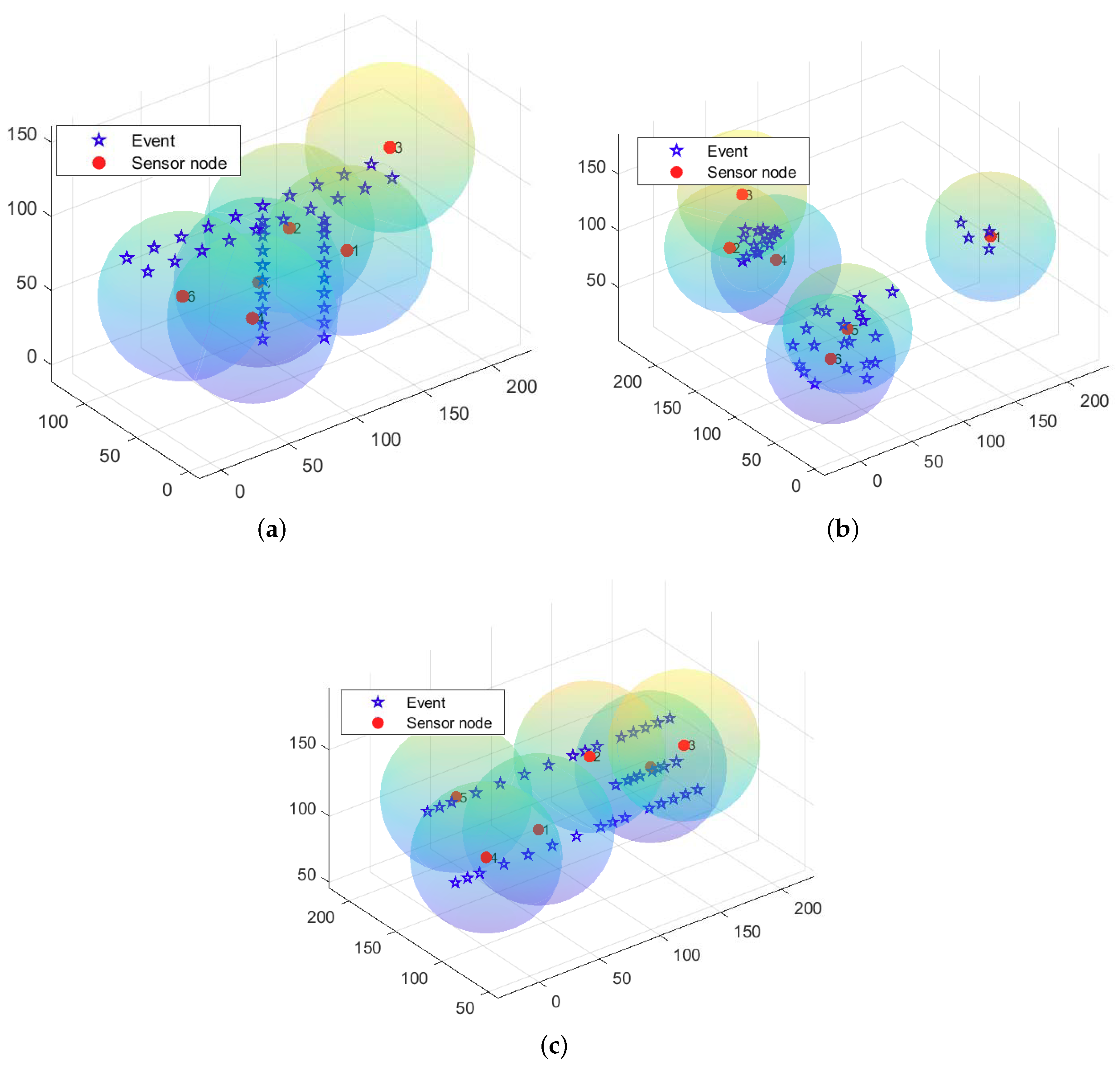
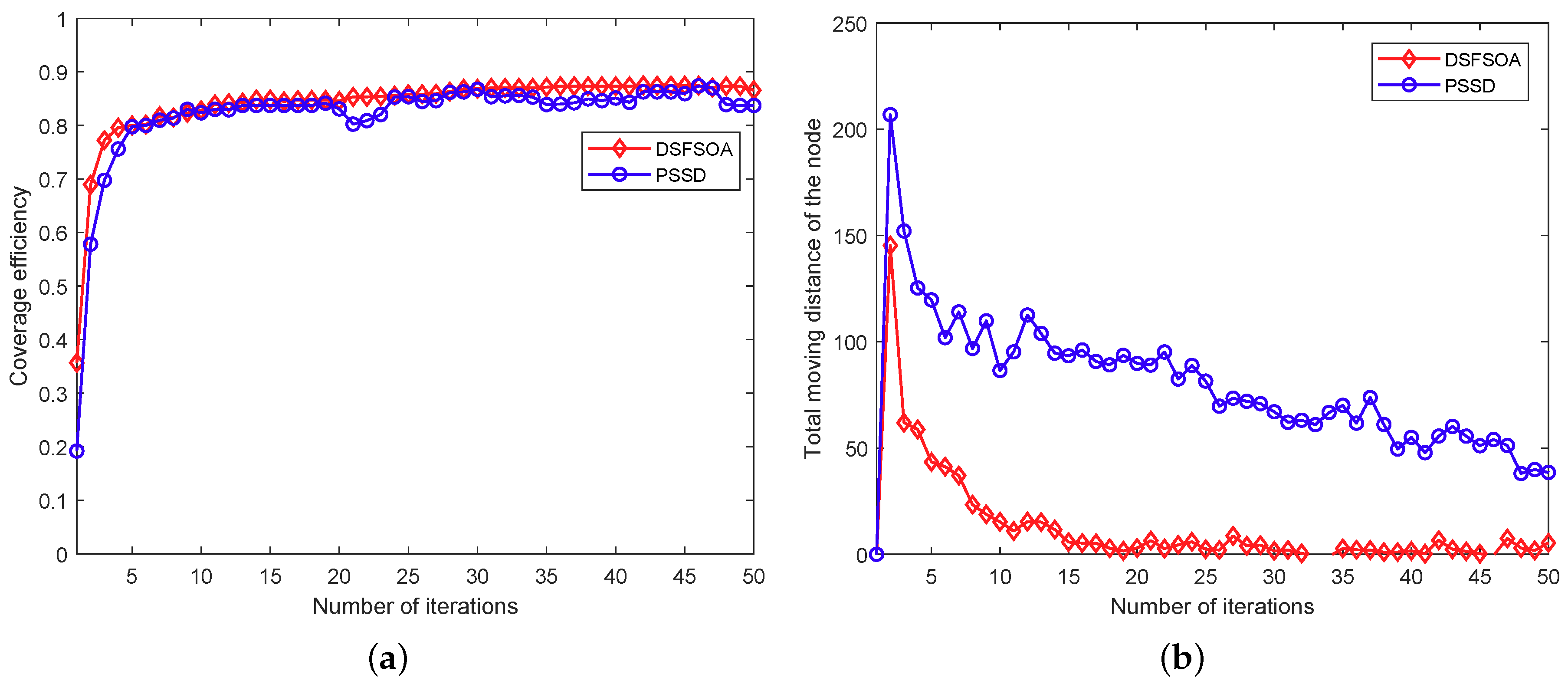
5.1. Static Environment Sensor Deployment

Three sets of experiments were implemented in a three-dimensional monitoring area of 200 m × 200 m × 200 m: (1) six sensor nodes and 40 events were unevenly distributed in a T shape; (2) six sensor nodes and 40 events were randomly distributed; and (3) six sensor nodes and 40 events were unevenly distributed in a line.
Figure 6 shows the results of the DSFSOA algorithm for self-organizing deployment of nodes. The light blue sphere represents the three-dimensional sensing range of the sensor node (the red center of the sphere is the position of the node), and the blue star represents the event. It can be seen that the DHFSOA algorithm is capable of achieving a final state in which all events covered by nodes and there is a good match between node distribution density and event distribution density.
The PSSD algorithm and the DHFSOA were used to deploy the sensor nodes. Figure 7 shows the evolution of the total moving distance and event coverage for the two algorithms in the three experiments. It should be noted that the final result for each set of experiments here is the average of 30 experiments. It can be seen in Figure 7a,c,e that the DHFSOA algorithm not only achieved high coverage of the event, but indeed achieved optimal coverage after just a few moves of the node, demonstrating faster convergence speed than the PSSD. More critically, the DHFSOA algorithm overcame the node blindness found in the traditional heuristic random search algorithm, while the PSSD algorithm exhibited significant instability and a poor final result. Figure 7b,d,f, is a comparison of the trend of the total moving distance of the node with the change of the number of iterations of the DSFSOA algorithm and the PSSD. It is clear that the DHFSOA algorithm greatly decreases the total moving distance of nodes during deployment compared with the PSSD algorithm. This is mainly due to the fact that the nodes in the PSSD algorithm make blind movements. The DHFSOA algorithm utilizes information sharing between the nodes based on the information pool. This improves the global sensing ability of the distributed fish swarm algorithm and thus avoids the blind movement of nodes, thereby reducing the total moving distance of nodes during deployment.

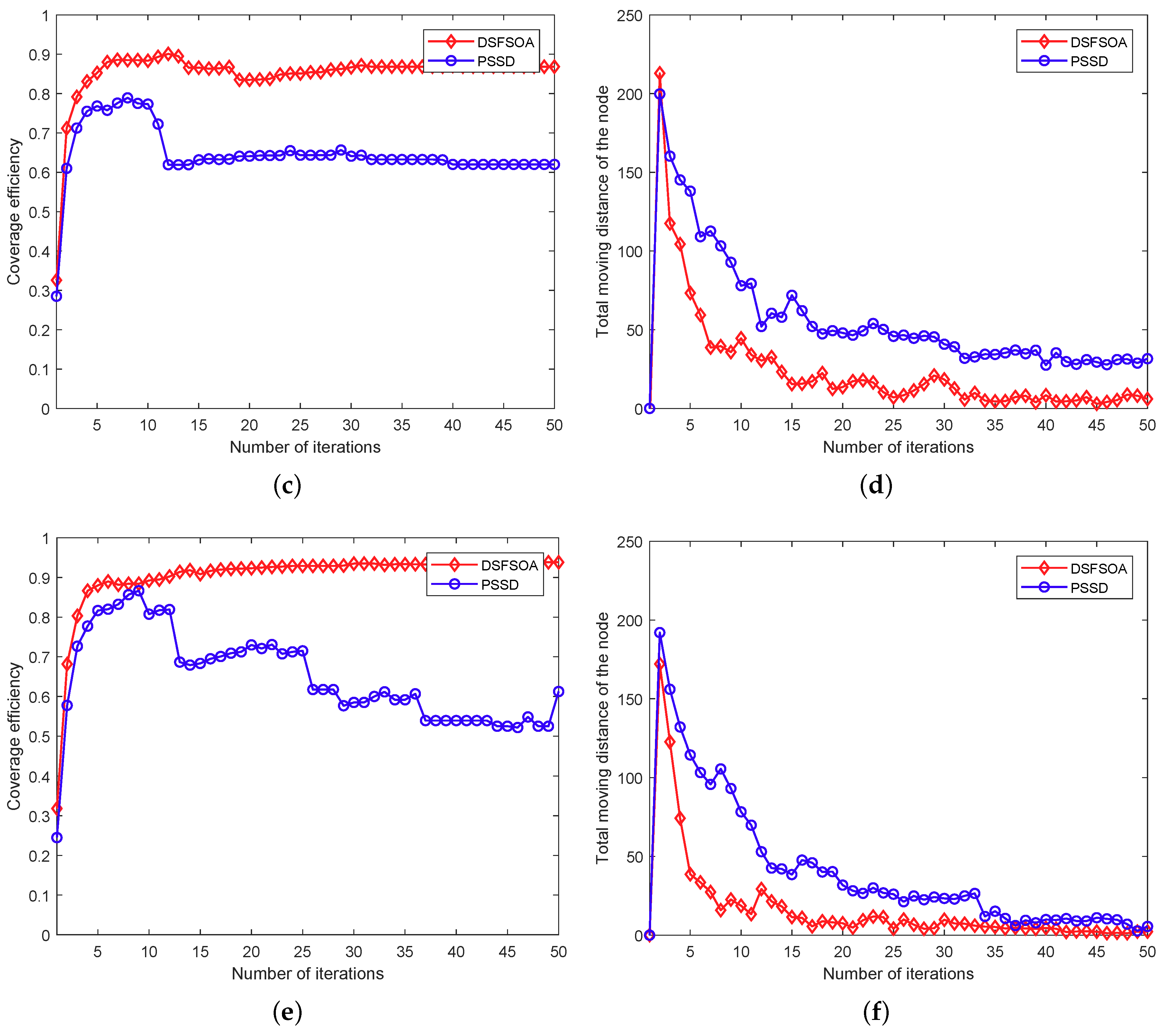
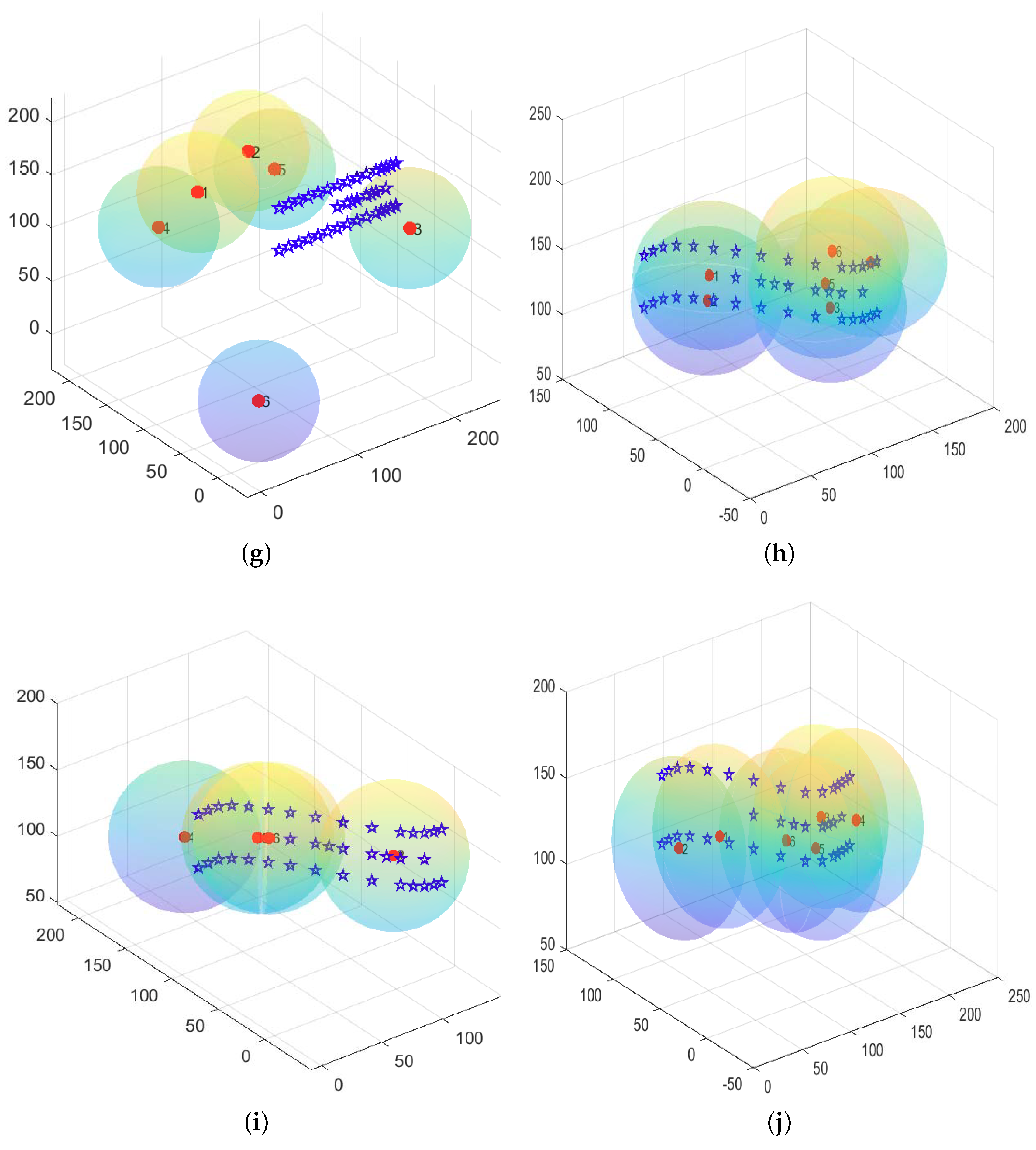
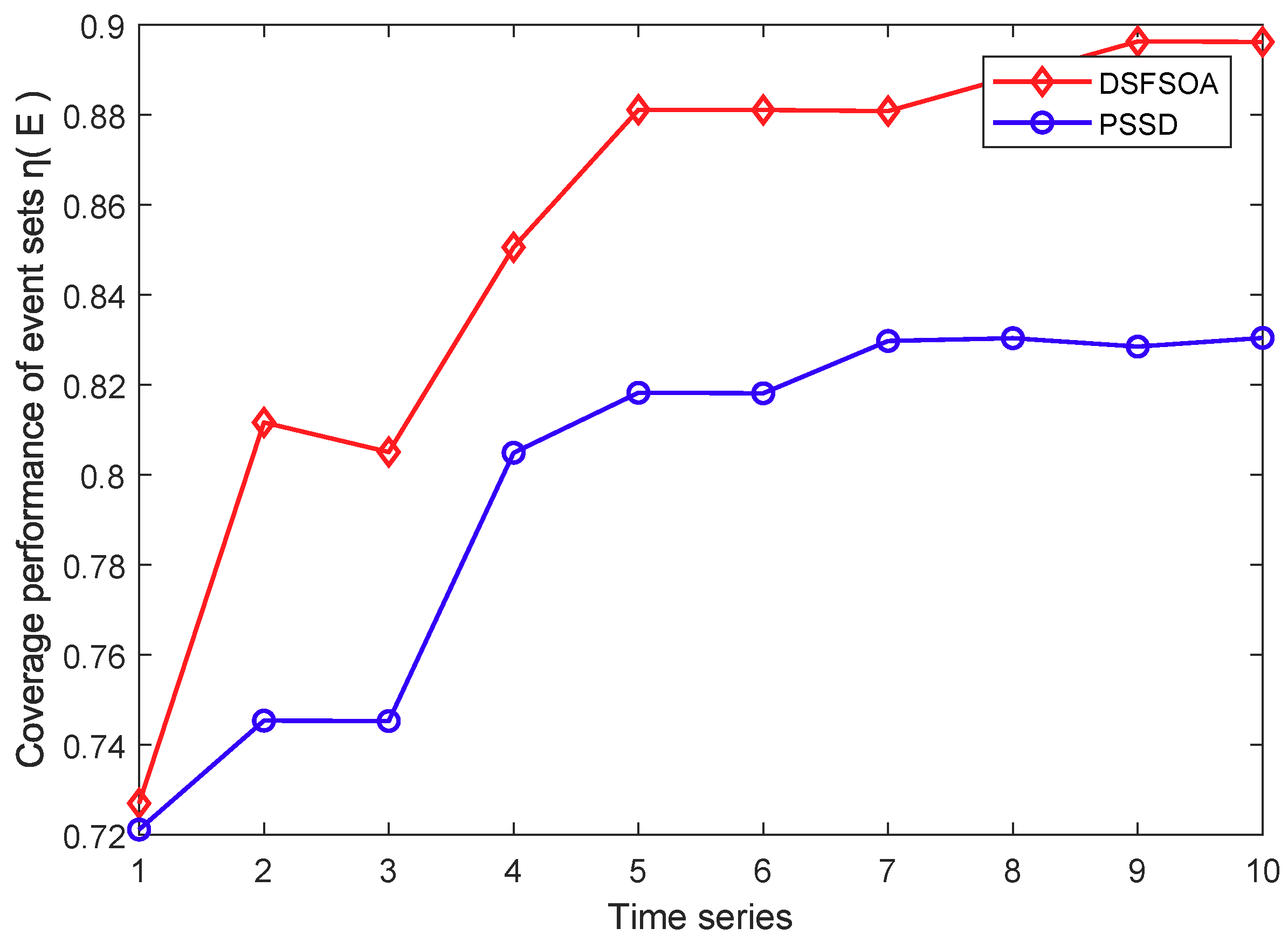
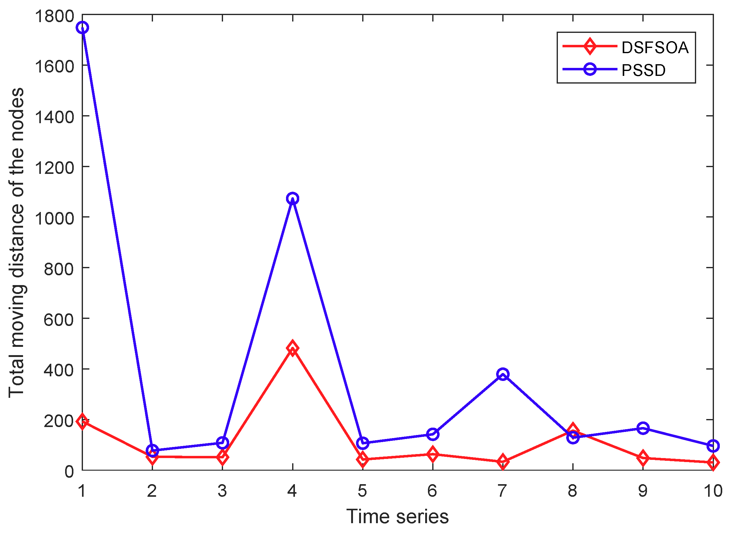
5.2. Sensor Deployment in a Dynamic Environment

To analyze the reliability and adaptability of the DHFSOA algorithm, this section explores the results of sensor deployment in a non-uniformly covered, dynamic ocean environment. Water flow velocity was generated based on a model presented in a previous study [19,24]; model parameters are listed in Table 2. The update period T for sensors in the DHFSOA was 0.5 s.
For the case in which events take place in a dynamic ocean environment, flowing water will cause their positions to change. The simulation results at four different times are shown in Figure 8a–d. As can be seen in the figures, when events present a linear distribution, underwater nodes also exhibit a linear distribution, and regions with high event densities have more underwater nodes. It can be seen that underwater nodes move with events and always present the same distribution shape. The node covers the events well, and achieves the matching of underwater node density and event density.
Next, the network operation time was divided into 10 segments. Figure 9 and Figure 10 respectively compare the coverage efficacy of the event set and the evolution of the total moving distance of the nodes during each monitoring period. It can be seen in Figure 8 that the coverage efficacy of the event set is constantly changing with time, and both the DHFSOA and PSSD algorithms maintain good states. The DHFSOA, however, dynamically adjusts quickly and is slightly better than the PSSD algorithm. Figure 9 is a comparison diagram between the PSSD algorithm and the DHFSOA for the changes in total node moving distance during the network running time. It can be seen that, compared with the PSSD, the DHFSOA algorithm greatly reduces the total moving distance of the nodes during the network operation, thus reducing total energy consumption. This allows the nodes to retain more energy, which can be used to participate in other tasks, effectively extending the network life cycle.
We can see from the preceding figures that, compared to the PSSD algorithm, the DHFSOA has obvious advantages in terms of network coverage, coverage efficacy of event sets, and total moving distance of nodes. This is due to that fact that, during network operation, the DHFSOA constructs an information pool, expands the nodes’ field of vision, enhances information sharing between nodes in the network connectivity state, avoids blind movement of nodes, and retains the global search ability of the traditional fish swarm heuristic algorithm.

6. Conclusions

This paper has proposed a distributed hybrid fish swarm optimization algorithm (DHFSOA) in order to optimize the deployment of underwater acoustic sensor nodes. The proposed DHFSOA was inspired by the artificial fish swarm operation system designed to simulate the preying, following, and swarming behaviors of fish. Applying these sorts of behaviors to sensor nodes gives them the autonomous tendency and ability to cover events within a monitoring area. Congestion distribution control was used to match node and event distribution densities. In addition, by constructing an information pool, the DHFSOA not only overcame the blindness of the traditional artificial fish swarm heuristic algorithm random search, but also retained the global search ability of the traditional fish swarm heuristic algorithm.
The proposed algorithm was evaluated by running a large number of comparative simulation experiments. Once the static and dynamic environments of the underwater acoustic sensor networks (UASNs) were established, the proposed DHFSOA was used for actual testing. The simulation results showed that the DHFSOA has the following three advantages over the PSSD algorithm: (1) the DHFSOA can maintain higher event coverage and coverage efficacy of event sets; (2) the DHFSOA can avoid blind movement of nodes, thus reducing total node moving distance and thereby reducing total energy consumption during node deployment; and (3) DHFSOA is a distributed algorithm, which shows strong extensibility during node deployment. In our next study, we will improve the proof of DHFSOA convergence and begin experimenting in actual underwater environments.

Author Contributions

H.W. and Y.L. conceived and designed the whole procedure of this paper. T.C. contributed to the introduction and system model sections. S.C. and Y.F. performed and analyzed the computer simulation results.

Funding

This research was supported by the National Natural Science Foundation of China (61571250), the Zhejiang Natural Science Foundation (LY18F010010), the Key Laboratory of Mobile Network Application Technology of Zhejiang Province, the K. C. Wong Magna Fund of Ningbo University, the Youth Project of Ningde Normal University (2017Q105,018Q103), the Teaching Reform Project of the Ningde Normal University (JG20180122), the project of the Education Department of Fujian Province (JT180596) and the project of the Fujian Provincial Natural Science Fund (2017I0016, 2017J01775).

Conflicts of Interest

The authors declare no conflict of interest.

References

  1. Akyildiz, I.F.; Pompili, D.; Melodia, T. Underwater acoustic sensor networks: Research challenges. Ad Hoc Netw. 2005, 3, 257–279. [Google Scholar] [CrossRef]
  2. Chen, K.; Ma, M.; Cheng, E.; Yuan, F.; Su, W. A survey on MAC protocols for underwater wireless sensor networks. IEEE Commun. Surv. Tutor. 2014, 16, 1433–1447. [Google Scholar] [CrossRef]
  3. Davis, A.; Chang, H. Underwater wireless sensor networks. In Proceedings of the IEEE Oceans 2012, Hampton Road, VA, USA, 14–19 October 2012; pp. 1–5. [Google Scholar]
  4. Berger, C.R.; Zhou, S.L.; Willett, P.; Liu, L.B. Stratification Effect Compensation for Improved Underwater Acoustic Ranging. IEEE Trans. Signal Process. 2008, 56, 3779–3783. [Google Scholar] [CrossRef] [Green Version]
  5. Wang, C.; Lin, H.; Jiang, H. CANS: A Congestion-Adaptive WSN-Assisted Emergency Navigation Algorithm with Small Stretch. IEEE Trans. Mob. Comput. 2016, 15, 1077–1089. [Google Scholar] [CrossRef]
  6. Wang, H.; Li, Y.; Chang, T.; Chang, S. An Effective Scheduling Algorithm for Coverage Control in Underwater Acoustic Sensor Network. Sensors 2018, 18, 2512. [Google Scholar] [CrossRef] [PubMed]
  7. Ian, F. Wireless sensor networks in challenged environments such as underwater and underground. In Proceedings of the 17th ACM International Conference on Modeling, Analysis and Simulation of Wireless and Mobile Systems, New York, NY, USA, 21–26 September 2014; pp. 1–2. [Google Scholar]
  8. Yang, X.; Miao, P.; Gibson, J.; Xie, G.G.; Du, D.Z.; Vasilakos, A.V. Tight performance bounds of multihop fair access for MAC protocols in wireless sensor networks and underwater sensor networks. IEEE Mob. Comput. 2011, 11, 1538–1554. [Google Scholar]
  9. Luo, X.; Feng, L.; Yan, J.; Guan, X. Dynamic Coverage with Wireless Sensor and Actor Networks in Underwater Environment. IEEE/CAA J. Autom. Sin. 2015, 2, 274–281. [Google Scholar]
  10. Liu, L.F. A deployment algorithm for underwater sensor networks in ocean environment. J. Circuits Syst. Comput. 2011, 20, 1051–1066. [Google Scholar] [CrossRef]
  11. Abo-Zahhad, M.; Ahmed, S.M.; Sabor, N.; Sasaki, S. Rearrangement of mobile wireless sensor nodes for coverage maximization based on immune node deployment algorithm. Comput. Electr. Eng. 2015, 43, 76–89. [Google Scholar] [CrossRef]
  12. Hua, C.B.; Wei, Z.; Nan, C.Z. Underwater Acoustic Sensor Networks Deployment Using Improved Self-Organize Map Algorithm. Cybern. Inf. Technol. 2014, 14, 63–77. [Google Scholar] [CrossRef] [Green Version]
  13. Bonabeau, E.; Dorigo, M.; Theraulaz, G. Swarm Intelligence: From Natural to Artificial Systems; Oxford University Press, Inc.: New York, NY, USA, 1999. [Google Scholar]
  14. Liu, X. Sensor deployment of wireless sensor networks based on ant colony optimization with three classes of ant transitions. IEEE Trans. Commun. Lett. 2012, 16, 1604–1607. [Google Scholar] [CrossRef]
  15. Wang, H.B.; Fan, C.C.; Tu, X.Y. AFSAOCP: A novel artificial fish swarm optimization algorithm aided by ocean current power. Appl. Intell. 2016, 45, 1–16. [Google Scholar] [CrossRef]
  16. Iyer, S.; Rao, D.V. Genetic algorithm based optimization technique for underwater sensor network positioning and deployment. In Proceedings of the 2015 IEEE Underwater Technology (UT), Chennai, India, 23–25 February 2015; pp. 1–6. [Google Scholar]
  17. Wang, Y.; Liao, H.; Hu, H. Wireless Sensor Network Deployment Using an Optimized Artificial Fish Swarm Algorithm. In Proceedings of the International Conference on Computer Science and Electronics Engineering, Hangzhou, China, 23–25 March 2012; pp. 90–94. [Google Scholar]
  18. Dhillon, S.S.; Chakrabarty, K. Sensor placement for effective coverage and surveillance in distributed sensor networks. In Proceedings of the Wireless Communications and Networking, New Orleans, LA, USA, 16–20 March 2003; pp. 1609–1614. [Google Scholar]
  19. Du, H.; Na, X.; Rong, Z. Particle Swarm Inspired Underwater Sensor Self-Deployment. Sensors 2014, 14, 15262–15281. [Google Scholar] [CrossRef] [PubMed] [Green Version]
  20. Das, S.; Liu, H.; Nayak, A. A localized algorithm for bi-connectivity of connected mobile robots. Telecommun. Syst. 2009, 40, 129–140. [Google Scholar] [CrossRef]
  21. Zhang, H.H.; Hou, J.C. Maintaining Sensing Coverage and Connectivity in Large Sensor Networks. Ad Hoc Sens. Wirel. Netw. 2005, 1, 89–124. [Google Scholar]
  22. Ghosh, A.; Das, S.K. Coverage and connectivity issues in wireless sensor networks: A survey. Pervasive Mob. Comput. 2008, 4, 303–334. [Google Scholar] [CrossRef]
  23. Neshat, M.; Sepidnam, G.; Sargolzaei, M.; Toosi, A.N. Artificial fish swarm algorithm: A survey of the state-of-the-art, hybridization, combinatorial and indicative applications. Artif. Intell. Rev. 2014, 42, 965–997. [Google Scholar] [CrossRef]
  24. Caruso, A.; Paparella, F.; Vieira, L.F.M.; Erol, M.; Gerla, M. The Meandering Current Mobility Model and its Impact on Underwater Mobile Sensor Networks. In Proceedings of the IEEE INFOCOM 2008, Phoenix, AZ, USA, 13–18 April 2008; pp. 771–775. [Google Scholar]
Figure 1. Flow chart of the artificial fish swarm algorithm.
Applsci 08 01638 g001
Figure 2. Concept of artificial fish vision.
Applsci 08 01638 g002
Figure 3. An example of information pool construction (there is an isolated node s 5 ).
Applsci 08 01638 g003
Figure 4. An example of information pool construction (no isolated nodes).
Applsci 08 01638 g004
Figure 5. Selection of relevant parameters of the moving step in the DSFSOA(distributed hybrid fish swarm optimization algorithm) algorithm. (a) the relationship between parameter k, g and a when I t e r is 20 and I t e r N u m is 50; (b) the relationship between a and I t e r when k = 20 and g = 5.
Applsci 08 01638 g005
Figure 6. Achievement of self-organized Deployment of Nodes using the DHFSOA. (a) events unevenly distributed in a T shape; (b) 40 events randomly distributed; (c) 40 events unevenly distributed linearly.
Applsci 08 01638 g006
Figure 7. Comparison of the evolution of total moving distance and event coverage of two methods in three sets of experiments. (a) Experiment 1: average coverage; (b) Experiment 1: total moving distance of nodes; (c) Experiment 2: average coverage; (d) Experiment 2: total moving distance of nodes; (e) Experiment 3: average coverage; (f) Experiment 3: total moving distance of nodes.
Applsci 08 01638 g007aApplsci 08 01638 g007b
Figure 8. The distribution of sensor nodes and events at times t 1 to t 4 . (a) initial time node t 1 and event distribution; (b) initial time node t 2 and event distribution; (c) initial time node t 3 and event distribution; (d) initial time node t 4 and event distribution.
Applsci 08 01638 g008
Figure 9. Comparison of the evolution of coverage efficacy at different times.
Applsci 08 01638 g009
Figure 10. Comparison of the evolution of the total moving distance of nodes at different times.
Applsci 08 01638 g010
Table 1. Simulation parameters.
ParameterValueParameterValue
Node’s radius of perception r s 50 mMaximum number of iterations T m a x 50
Node’s radius of communication r c 100 mConstant N m a x 5
Length of moving step l15 mConstant ψ 0.1
Table 2. Parameters of the dynamic ocean environment.
ParameterThe Water Flow FieldTarget Number
kc av ε ω SensorsEvents
Value 2 π 7 . 5 0.121.20.30.4640

