Research on Reliability Assessment of Mechanical Equipment Based on the Performance–Feature Model

Abstract

There is a growing body of literature which recognizes the importance of mechanical equipment reliability during processing, and reliability assessment is important in guaranteeing the precision, function, and use life span of mechanical equipment. For products with a long lifetime and high reliability, it is difficult to assess lifetime and reliability using traditional statistical inference based on a large sample of data from the lifetime test. Therefore, this study contributed to this growing area of research, through a reliability evaluation method based on degradation path distribution related to signal characteristics. In this research, an effective method for reliability assessment was constructed, in which the signal features of the machining process were used to replace traditional time data and fit equipment degradation model. The pseudo failure characteristic (PFC) was obtained according to the failure threshold and the reliability curve was plotted by a PFC distribution model. Experimental investigation on tool reliability assessment was used to verify the effectiveness of this method, in which the trend that tool wear changes with the features was fitted by a Gaussian distribution function and Logarithmic distribution function, to obtain a better tool degradation model. The results illustrated the model could evaluate reliability of mechanical equipment effectively.

1. Introduction

Reliability assessment for mechanical equipment is important in condition-based maintenance to lower cost and improve equipment reliability, thus, it emerges repeatedly and has become an important research area for mechanical equipment reliability analysis and life prediction [1,2,3]. Z.M. Wang [4] proved that the bounded intensity process was suitable for reliability assessment of deterioration in machine tools with frequent maintenance actions. How to assess reliability is also helpful for predictive life [5] and maintenance time [6]. Performance degradation is one of the most important elements during machining, which has a close relationship with product precision, by influencing the total manufacturing effectiveness and stability of machine tools. In most circumstances, performance degradation is the main failure for mechanical equipment and leads to the waste of product and time. In addition, equipment condition is closely related to a machine’s efficiency and productivity, therefore, research on reliability assessment of mechanical equipment is important, based on performance degradation analysis [7].

As an important concern during processing, several studies are being conducted by many researchers for reliability assessment. The traditional reliability evaluation method is usually based on the failure life data [8], and the failure life time is obtained through the life test and accelerated life test. The main function of the reliability life test is to process indiscriminate failure life data and realize the reliability evaluation of the product through the test, which cannot effectively understand product failure process and failure mechanism and cannot contribute to product reliability growth. Traditional reliability analysis is based on the probability statistics method for the failure data from a large sample, so failure data with a small sample is difficult to effectively analyze. For high reliability and long-life products, it is difficult to get failure life time through the life test and accelerated life test. Therefore, there are many new reliability evaluation methods. F. Kuang [9,10] proposed a new reliability evaluation model based on quality loss and quality characteristics evolution. H.K. Li [11] studied the tool reliability evaluation based on acoustic emission signals. Meanwhile, this equipment performance degradation data can provide important information for reliability evaluation, thus, two reliability evaluation methods based on performance degradation data were presented, i.e., reliability evaluation method based on degradation path and reliability evaluation method based on performance degradation distribution [12,13]. The reliability estimation approaches of mechanical equipment are based on the historical performance degradation data, amongst which statistical distribution models [14] have been used in this area, such as the regression model [15], exponential distribution, and Weibull distribution [8,16,17,18]. In this research, a novel method for reliability assessment of mechanical equipment based on process signals and degenerate data was developed. Performance degradation data and process signals for mechanical equipment were used fit the degradation path for reliability assessment. This kind of method depended on sizable historical data and sensor signals from related equipment, and an experiment data set of tool wear was used to verify the effectiveness of the method. The results showed that this method could benefit reliability assessment. This paper was structured as follows. Section 2 introduced some basic theories of this method and the flow path in detail. Section 3 provided a general process of reliability assessment based on degradation paths. Section 4 used experimental data to verify the method. In this section, the feasibility and practicability of this method were proved. Concluding remarks were given in Section 5.

2. Theory

2.1. Method Flowchart

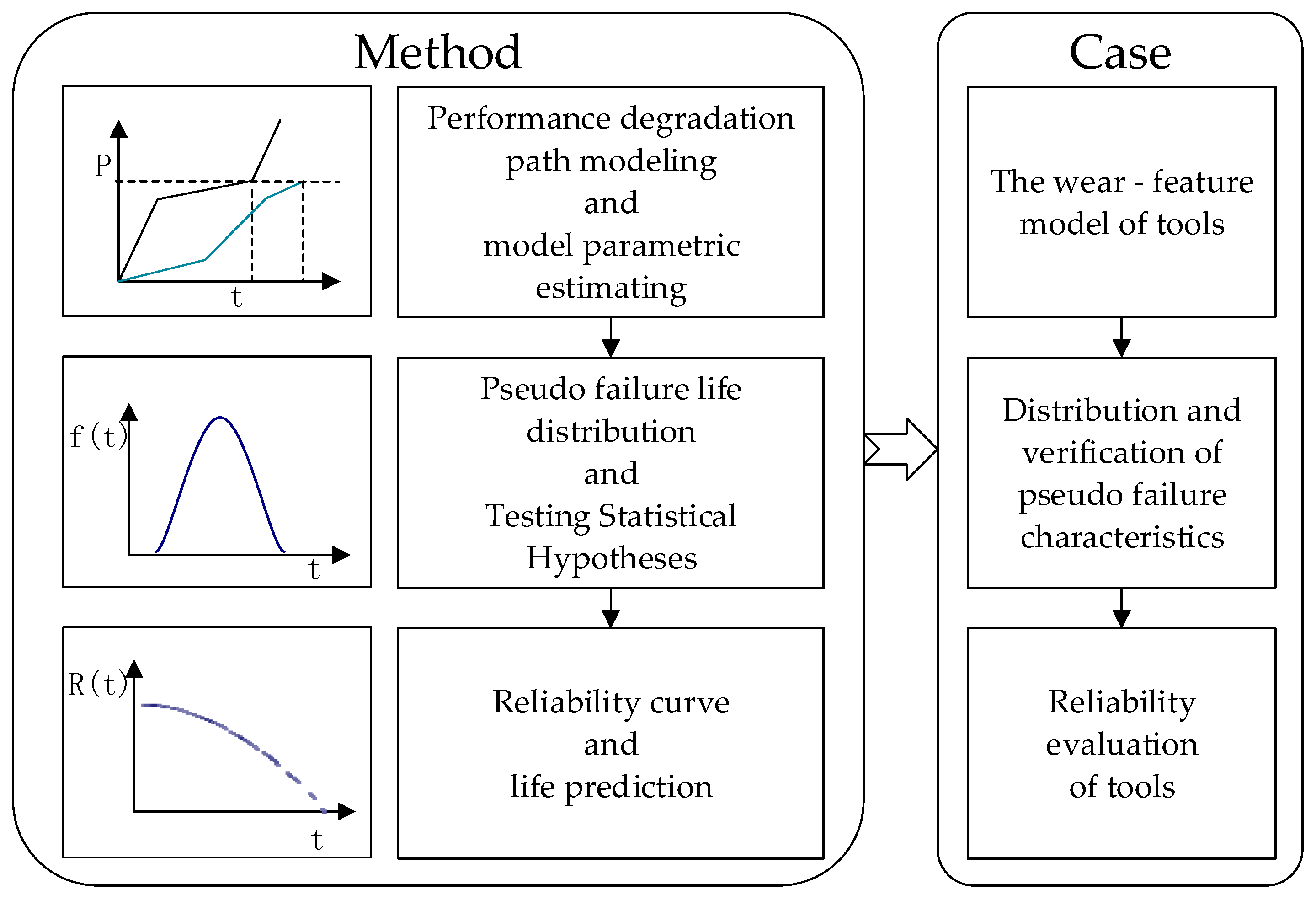
In this paper, the features of monitored vibration signals were extracted and the performance degradation data was applied to reliability assessment for mechanical equipment. The process of method is shown in Figure 1.

There are three main parts, i.e., performance degradation path modeling and model parametric estimating, pseudo failure life distribution and Testing Statistical Hypotheses, and reliability curve and life prediction. The first part is the performance degradation path modeling and model parametric estimating, where the performance degradation data of samples are known to fit the degradation path using the features extracted from processing signals, and the model parameters that reflect the degradation paths of different samples are calculated. The second part is pseudo failure life distribution and Testing Statistical Hypotheses. Pseudo failure characteristics (PFCs) are collected based on threshold values and the performance degradation model, and the distribution of the feature is extracted and verified by Testing Statistical Hypotheses. The third part is reliability curve and life prediction, i.e., the reliability curve is plotted, and the characteristics of different reliability can be obtained. In the end, an example for tool analysis is investigated in this research to verify the effectiveness of the method.

2.2. Basic Concepts of Performance Degradation

In the reliability degradation test, it is difficult to continuously monitor the degradation process of product performance, so the performance characteristics of the product can be tested regularly in the test process. The amount of performance degradation recorded, contains a lot of useful information about product performance degradation and reliability [19,20].

For some products with obvious performance degradation characteristics, the degradation mechanism is easy to understand, so product reliability can be directly derived by using the relationship between degradation characteristics and time [21]. For products with performance degradation characteristics that are not obvious, the quantitative relationship of the degradation model cannot be directly expressed, and analysis methods and techniques such as regression analysis are needed. In many cases, the degradation model of products is often a nonlinear function of the parameters, and the calculation of the parameters of such models is often very large.

Assuming that the regression paths of the samples satisfy the model, the times at which the different samples reach the failure threshold can be deduced. Since these times are not the actual failure times of the samples, using them to evaluate product reliability is needed, so it is called pseudo failure life time. The life time of each sample can be predicted, that is, the life distribution of the product.

Relative to the failure time data, the reliability of the product performance degradation data contains more information. In addition, through the product performance degradation information, reliability analysis can be time and cost effective. Reliability analysis based on performance degradation data will be one of the methods used to evaluate the reliability of high reliability and long-life products.

The use of degradation data, instead of failure time data, for product reliability life assessment has the following advantages:

(1) For many products, degradation is a natural attribute and its performance data can be monitored to obtain degradation data regardless of failure;

(2) Degraded data can be applied in cases where there are only a few or zero failures, which can provide more information than failure time data;

(3) The degraded data can provide more accurate life estimation, than the accelerated life test with little or no failure. In other words, for products with zero failure, useful reliability inferences can be obtained using degraded data.

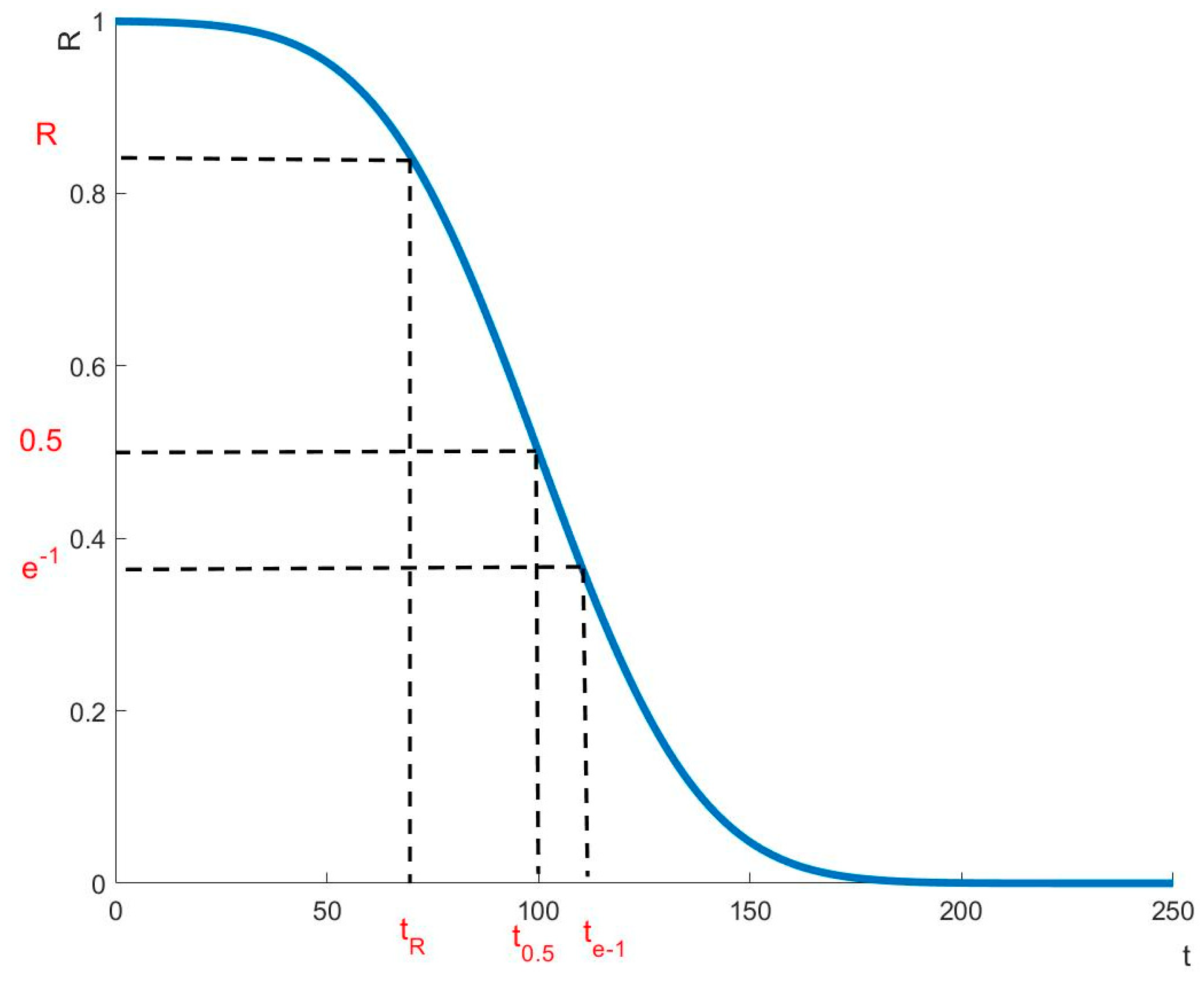
If degradation performance reaches a critical level, which can be defined as the failure threshold D_f, the failure will occur, then the product fault time T can be defined as the time that actual degradation path D(t) reached the critical degradation level D_f. The degradation paths of different products are random, and the time of the degradation critical level will be also different from one product to another product, so the random distribution can be used to describe the degradation and to establish the model. Then this model can reflect the model parameters. Therefore, the product failure time distribution can be derived by the degenerate data model, describing the relationship between D(t) and D_f.

3. Method

3.1. Performance Degradation Path Modeling and Model Parametric Estimating

For some obvious traits of performance degradation products, degradation mechanisms are easy to understand, one can use the relationship between the degradation characteristics and time to calculate the reliability of the product. For products with performance degradation characteristics are not obvious, the quantitative relationship of the degradation model cannot be directly expressed, and analysis methods and techniques such as regression analysis are needed. Therefore, the reliability evaluation method based on the degraded path is proposed, as described in Reference [15].

Firstly, the performance degradation data of the products at different times are collected, which do not have to reach the failure threshold, and the features associated with performance degradation from monitored signals are extracted and used to replace time. Then, the appropriate degradation model according to the performance degradation curve trend is selected. Different distributions, as the alternatives, are chosen to match the relationship between the feature value and performance degradation value. Linear, exponential, and Gaussian distribution are usually chosen as the degradation model, as outlined in Reference [19]. Different distributions will also be discussed depending on the features extracted.

Linear distribution can be expressed by Equation (1).

$$f_{Linear}(x)=ax+b$$

(1)

Exponential distribution can be expressed by Equation (2).

$$f_{Exponent}(x)=a·e^{bx}$$

(2)

Gaussian distribution can be expressed by Equation (3).

$$f_{Guassian}(x)=a·e^{(-{(\frac{x-b}{c})}^2)}$$

(3)

where a, b, and c are estimators of the distribution parameters and are different in different sample modeling. So, the parameters of each performance degradation model are estimated according to the recorded performance degradation data.

3.2. Pseudo Failure Characteristics Distribution and Testing Statistical Hypotheses

Assuming the failure threshold is D_f and according to the obtained sample degradation model f(x), in which x is defined as an independent variable that records performance degradation data and can be time, signal characteristics, etc., the characteristic of each sample arriving at the threshold is deduced, which is called the PFC. PFC data will follow the distribution of the failure characteristic. The failure life of high reliability and long-life products generally follows Weibull distribution, logarithmic normal distribution, or Gaussian distribution.

Primarily, we suppose that PFCs follow a distribution $F(x)$, and $F_0(x)$ is a completely determined continuous distribution function. Consider the hypothesis testing problem,

$${\mathrm{H}}_0:F(x)=F_0(x)$$

(4)

For example, the PFCs follow an exponential distribution $F_0(x)=1-e^{-{(x/\theta )}^2}$, and the parameter θ can be obtained by maximum likelihood estimation, which is equal to the average of the samples. Namely, the PFC values of the products need to be proven to follow one-parameter exponential distribution parameter of θ.

Samples $X_1,X_2,\cdots ,X_n$ are taken and the sample size is n, and their sequential statistics are $X_1\le X_2\le \cdots \le X_n$. Arrange the samples to get their empirical distribution function $F_n(x_i)$ and calculate ${\delta }_i$,

$$F_n(x_i)=\{\begin{array}{cc}0,& x\le X_i\\ i/n,\hspace{0.17em}\hspace{0.17em}& X_i\le x<X_{i+1}\\ 1,& x\ge X_n\end{array}$$

(5)

${\delta }_i$ is calculated by Equation (6).

$${\delta }_i=max\left\{\left|F_0(x_i)-(i-1)/n\right|,\left|F_0(x_i)-i/n\right|\right\},\hspace{0.17em}i=1,2,\cdots ,n$$

(6)

Kolmogorov-Smirnov (KS) test parameters are listed in

Table 1. Kolmogorov-Smirnov (KS) test table.

$\mathit{i}$	${\mathit{x}}_{\mathit{i}}$	${\mathit{F}}_{\mathbf{0}}\mathbf{\left(}{\mathit{x}}_{\mathit{i}}\mathbf{\right)}$	$\mathbf{\left(}\mathit{i}\mathbf{-}\mathbf{1}\mathbf{\right)}\mathbf{/}\mathit{n}$	$\mathit{i}\mathbf{/}\mathit{n}$	${\mathit{\delta }}_{\mathit{i}}$
1
2
3
⋮ ⋮
n

:

In this table, $x_i$ is the PFC of number i. The biggest ${\delta }_i$ is $D_n$, and that is,

$$D_n=\underset{i}{\max }\left\{{\delta }_i\right\}$$

(7)

Giving the significance level α, the critical value $d_{n,\alpha }$ can be obtained by looking up the critical value table of the Kolmogorov test, if $D_n<d_{n,\alpha }$, it follows the hypothesis ${\mathrm{H}}_0$. Otherwise, the hypothesis is rejected.

3.3. Reliability Curve and Life Prediction

The PFC data obtained above are regarded as the complete life data, and the product is evaluated according to the reliability evaluation method of the selected characteristic distribution.

Reliability [22] is the probability that the product will complete the specified function within the specified time and under the specified conditions, which is denoted as R. The reliability that a function of time, R(t), is called the reliability function. In this paper, reliability can be expressed as a function R(c) that changes with the extracted characteristics. If the failure time of the device is represented by the random variable T, the reliability function R(t) of the device will be

$$R(t)=P(T>t)={\int }_t^{+\infty }f(t)dt$$

(8)

where $f(t)$ is the probability density function, because the cumulative failure probability function $F(t)$ is

$$F(t)=P(T\le t)$$

(9)

From Equations (8) and (9), it is easy to get:

$$R(t)=1-F(t)$$

(10)

It can be seen from the expression of the reliability function R(t), that the reliability R of the device decreases with the increase in service time. This is because with the increase in service time, wear phenomenon appears in the equipment. Thus, the failure rate of the equipment increases, resulting in the decrease of reliability.

There is a one-to-one correspondence between reliability function and working time. When the reliability of the device is reduced to the given value R ($0\le \mathrm{R}\le 1$), the working time is called the reliability life of the reliability degree R, denoted as $t_R$, and the mathematical relationship is:

$$R(t_R)=\mathrm{R}$$

(11)

When the reliability is equal to 0.5, the corresponding eigenvalue is defined as the median eigenvalue, and when the reliability is equal to e⁻¹, the corresponding eigenvalue is defined as the reliable eigenvalue. The reliability curve is shown in Figure 2.

The reliability curve can be obtained according to the hypothesis. According to the reliability parameter formula of the product, the instantaneous loss efficiency, average loss efficiency, reliable life, median life, reliability, and average life of the product can be obtained.

4. Case Study

4.1. The Wear-Feature Model of Tools

Milling experimental data came from Li’s team at the Singapore Institute of Manufacturing Technology [23]. The data set contained tool wear and vibration signals of 315 cutting tests. Three piezo accelerometers were used to measure the machine tool vibrations of the cutting process in different directions, respectively. The machining tests were carried out with cutting speeds of 4.7 m/min and spindle speed 23,600 rpm. In this experiment, tool life-cycle experiments were made by inspecting the tool wear. The cutter’s wear was measured after a complete cutting distance using a LEICA MZ12 microscopy system (Leica Microsystems, Wetzlar, Germany). To decrease the influence of other factors on the vibration signals, the cutting parameters were same in the experiments for three samples. The collection frequency of experimental data was 50 KHz/channel.

In many components of cutting vibration, the influence of tool wear on the vibration is obvious. However, the cutting vibration increases with cutting tool wear, despite some fluctuation. It is mainly related to factors such as material properties, built-up edge, and measurement error, which accumulate in the cutting process. However, the influence on the overall upward trend of cutting vibration is small.

To show the feature trend with the number of milling significantly, vibration signals that had better linear relationships with the tool wearing process were decomposed, then the intrinsic mode functions (IMFs), frequency spectrums of IMFs, and the features relating to amplitude changes of frequency spectrum were obtained, thus feature value Gn, as outlined in Reference [18] could be calculated using

$$Gn(j)={\displaystyle \sum }_{f=11.2\mathrm{KHZ}}^{f=11.4\mathrm{KHZ}}{A}_j(f)j=1,2,\cdots ,P$$

(12)

where j is the number of cuts, and P = 315 in Figure 3. $A_j(f)$ shows the frequency spectrum amplitude of IMF1 decomposed from vibration signals at the jth milling in f Hz.

The results obtained from preliminary calculation of Gn in the milling process, are shown in Figure 3. Despite the fluctuations in the amplitude, the amplitude of Gn is expected to continue increasing with the number of cuts in the milling process; and the results of the correlational analysis between Gn and tool wear show that there is a high correlation between the feature value and the tool wear.

4.2. Distribution and Verification of Pseudo Failure Characteristics

Gaussian and Logarithmic distribution, as the alternatives, are chosen to calculate the parameters of distribution depending on the different models between the feature value and the tool wear.

Gaussian distribution can be expressed by Equation (3) and used in model A.

Logarithmic distribution can be expressed by Equation (13) and used in model B.

$$f_{Logarithm}(x)=a{\log }_{10}x+b$$

(13)

Table 2. Estimated parameters of Gaussian distribution.

Parameters	1	2	3	4	5	6	7	8	9
a	0.1722	0.1569	0.1514	0.2009	0.2442	0.2538	0.1709	0.2426	0.2425
b	5.074	4.673	3.708	10.9	12.01	13.35	13.37	17	14.22
c	5.105	4.964	3.736	9.267	9.384	10.66	15.6	15.78	12.54
Relevancy (RE)	0.8953	0.8552	0.7844	0.8513	0.8657	0.8352	0.8719	0.909	0.9422

and

Table 3. Estimated parameters of Logarithmic distribution.

Parameters	1	2	3	4	5	6	7	8	9
a	0.1065	0.0956	0.1047	0.1425	0.1641	0.1494	0.07859	0.1193	0.1447
b	0.093	0.0923	0.0911	0.0384	0.0308	0.0386	0.0788	0.06602	0.05503
RE	0.8746	0.8656	0.8171	0.8381	0.8252	0.7927	0.8901	0.8402	0.8863

show the parameter a, b, and c calculated for these samples’ distribution, and relevancy (RE) is shown in Table 2 and Table 3. As these tables show, the distribution fitting of model A and model B are highly correlated.

Assuming that the failure threshold of the cutting tool wear was 0.16 mm, according to the degradation model, we calculated the PFC of each failure threshold value. The results are shown in

Table 4. The pseudo failure characteristics (PFCs) of each sample.

Sample Number	1	2	3	4	5	6	7	8	9
Gaussian Distribution	6.46	5.37	4.59	15.32	18.11	20.59	17.37	27.18	22.31
Logarithmic Distribution	4.26	5.11	4.55	7.14	6.13	6.49	10.79	6.14	5.31

. From the chart, it can be seen that the PFCs obtained from Gaussian distribution were larger than those obtained from Logarithmic distribution.

Failure characteristics of cutting tools are assumed to be an exponential distribution, in which maximum likelihood estimation is calculated, and the goodness of fit test is done based on the Kolmogorov-Smirnov (KS) test.

Nine groups of samples were arranged to obtain their empirical distribution function and calculated ${\delta }_i$. The results are shown in

Table 5. Kolmogorov-Smirnov (KS) test of Gaussian distribution.

$\mathit{i}$	${\mathit{x}}_{\mathit{i}}$	${\mathit{F}}_{\mathbf{0}}\mathbf{\left(}{\mathit{x}}_{\mathit{i}}\mathbf{\right)}$	$\mathbf{\left(}\mathit{i}\mathbf{-}\mathbf{1}\mathbf{\right)}\mathbf{/}\mathit{n}$	$\mathit{i}\mathbf{/}\mathit{n}$	${\mathit{\delta }}_{\mathit{i}}$
1	4.59	0.2598	0	0.111	0.2598
2	5.37	0.2967	0.111	0.222	0.1857
3	6.45	0.3448	0.222	0.333	0.1228
4	15.32	0.6337	0.333	0.444	0.3007
5	17.37	0.6798	0.444	0.556	0.2358
6	18.11	0.6949	0.556	0.667	0.1389
7	20.59	0.7407	0.667	0.778	0.0737
8	22.31	0.7684	0.778	0.889	0.1206
9	27.18	0.8317	0.889	1	0.1683

and

Table 6. KS test of Logarithmic distribution.

$\mathit{i}$	${\mathit{x}}_{\mathit{i}}$	${\mathit{F}}_{\mathbf{0}}\mathbf{\left(}{\mathit{x}}_{\mathit{i}}\mathbf{\right)}$	$\mathbf{\left(}\mathit{i}\mathbf{-}\mathbf{1}\mathbf{\right)}\mathbf{/}\mathit{n}$	$\mathit{i}\mathbf{/}\mathit{n}$	${\mathit{\delta }}_{\mathit{i}}$
1	4.26	0.4963	0	0.111	0.4963
2	4.55	0.5193	0.111	0.222	0.4083
3	5.11	0.5607	0.222	0.333	0.3387
4	5.31	0.5746	0.333	0.444	0.2416
5	6.13	0.6272	0.444	0.556	0.1832
6	6.14	0.6278	0.556	0.667	0.0718
7	6.49	0.6482	0.667	0.778	0.1298
8	7.14	0.6832	0.778	0.889	0.2058
9	10.79	0.8239	0.889	1	0.1761

.

According to the critical value table, the critical value $d_{n,\alpha }$ was equal to 0.51332 at the 0.05 significance level, and $D_n$ can be obtained in Table 5 and Table 6. Since $D_n<d_{n,\alpha }$, both model A and model B followed the hypothesis of exponential distribution.

4.3. Reliability Evaluation of Tools

The PFCs obtained are regarded as complete failure characteristic data, and the tool was evaluated according to the reliability evaluation method of the exponential distribution. The reliability function of the model A is shown below:

$$R(c)=R_G(Gn)=e^{-Gn/15.2544}$$

(14)

Figure 4 shows a reliability curve that follows an exponential distribution.

When the reliability is equal to 0.5, the corresponding eigenvalue is defined as the median eigenvalue $G{n}_{R=0.5}$, and when the reliability is equal to $e^{-1}$, the corresponding eigenvalue is defined as the reliable eigenvalue $G{n}_{R={\mathrm{e}}^{-1}}$.It can be obtained by Formula (14) that,

$$G{n}_{R=0.5}=10.5735$$

$$G{n}_{R={\mathrm{e}}^{-1}}=15.2544$$

The number of cuts of tool wear limit, marked as N_t, and the number of cuts based on the characteristic value were found, then the number of cuts based on the median eigenvalue was marked as N_0.5, and the number of cuts based on the natural eigenvalue was recorded as N_e. The relative error between actual cutting times and estimated cutting times was calculated and used to validate the model and the method. The results are shown in

Table 7. The number of cuts corresponding to the failure threshold.

Sample Number	1	2	3	4	5	6
Nt	285	274	276	285	236	230
N0.5	>315	>315	>315	274	274	274
Ne	>315	>315	>315	>315	>315	>315

.

The estimated cutting times were higher than the test times, so the error was larger.

The reliability function of the model B is shown below:

$$R(c)=R_L(\mathrm{Gn})=e^{-Gn/6.212}$$

(15)

Figure 5 shows a reliability curve that follows an exponential distribution.

It can be obtained by Formula (15) that,

$$G{n}_{R=0.5}=4.306$$

$$G{n}_{R=e^{-1}}=6.212$$

The results of relative error and the number of cuts are shown in

Table 8. The number of cuts corresponding to the failure threshold.

Sample Number	1	2	3	4	5	6
Nt	285	274	276	285	236	230
N0.5	247	247	247	193	193	193
Relative Error (%)	13.3	9.8	10.5	32.3	18.2	16.1
Ne	270	270	270	238	238	238
Relative Error (%)	5.3	1.5	2.2	16.5	0.85	3.4

.

The relative error was concentrated between one and five percent, and the verification result was good, so compared with model A, model B was superior and more suitable to evaluate tool reliability.

5. Conclusions

This paper presented the reliability assessment method of mechanical equipment based on the performance degradation path, which was developed for reliability through exploring the relationship between signal characteristics and performance degradation. The signal characteristic correlated with the degradation of performance was obtained, then the estimation method based on the feature-performance model was more practical. Performance degradation path modeling can help to find performance degradation distribution fitting, and model parameter estimation shows the difference between the samples; then the Pseudo Failure Characteristics (PFCs) can be calculated based on the threshold gained from experience. Verification of PFC distribution indicated the validity of failure features, and the function describing the failure characteristic distribution was chosen to calculate the reliability curve. In this paper, a case study of tool wear was used to verify the method. The vibration signal characteristic Gn was proved to be highly correlated with tool wear. The wear-feature model that fits tool wear distribution was used to estimate model parameters of the different tools, then the PFCs were calculated based on the tool wear threshold that was set at 0.16 mm in this paper. Verification of failure characteristics indicated that Exponential distribution could be used to describe the characteristic distribution. Then, reliability curve and failure characteristic prediction could be obtained. In further work, the method can be used to calculate real-time estimate tool life and improve processing quality. The paper contributes to our understanding of performance degradation and provides a basis for reliability evaluation of mechanical equipment by the degradation path.

References

1. Bona, G.D.; Forcina, A.; Petrillo, A.; Felice, F.D.; Silvestri, A. A-IFM reliability allocation model based on multicriteria approach. Int. J. Qual. Reliab. Manag. 2016, 33, 676–698. [Google Scholar] [CrossRef]
2. Bona, G.D.; Silvestri, A.; Forcina, A.; Falcone, D. Ahp-IFM target: An innovative method to define reliability target in an aerospace prototype based on analytic hierarchy process. Qual. Reliab. Eng. Int. 2017, 33, 1731–1751. [Google Scholar] [CrossRef]
3. Bona, G.D.; Forcina, A.; Silvestri, A. Critical flow method: A new reliability allocation approach for a thermonuclear system. Qual. Reliab. Eng. Int. 2016, 32, 1677–1691. [Google Scholar] [CrossRef]
4. Wang, Z.M.; Yang, J.G. Bounded intensity process and its applications in reliability assessment of nc machine tools. J. Shanghai Jiaotong Univ. 2012, 46, 1623–1631. [Google Scholar]
5. Zhao, M.; Lin, J. Health assessment of rotating machinery using a rotary encoder. IEEE Trans. Ind. Electron. 2017, 65, 2548–2556. [Google Scholar] [CrossRef]
6. Wang, Z.M.; Yang, J.G.; Wang, G.Q.; Zhang, G.B. Reliability assessment of multiple NC machine tools with minimal repair. J. Harbin Inst. Technol. 2011, 43, 127–130. [Google Scholar]
7. Sung, S.I.; Yum, B.J. Optimal design of step-stress accelerated degradation tests based on the wiener degradation process. Qual. Technol. Quant. Manag. 2016, 13, 367–393. [Google Scholar] [CrossRef]
8. Dai, Y.; Zhou, Y.F.; Jia, Y.Z. Distribution of time between failures of machining center based on type I censored data. Reliab. Eng. Syst. Saf. 2003, 79, 377–379. [Google Scholar] [CrossRef]
9. Kuang, F.; Dai, W.; Chen, L.; Zhao, Y. Assessment method and applications for reliability manufacturing process based on quality loss. Comput. Integr. Manuf. Syst. 2015, 21, 1571–1578. [Google Scholar]
10. Kuang, F.; Dai, W.; Wang, J.; Zhao, Y. Process reliability evaluation based on quality characteristics evolution. Comput. Integr. Manuf. Syst. 2015, 21, 2124–2131. [Google Scholar]
11. Li, H.K.; Wang, Y.H.; Yang, S.H.; Zhao, P.S. Estimation of operational reliability for milling cutter based on acoustic emission signal. J. Dalian Univ. Technol. 2014, 54, 418–423. [Google Scholar]
12. Chao, D.; Jing, M.; Chen, S.; Zhang, C. Reliability assessment of fogs used for satellite from degradation data. Infrared Laser Eng. 2011, 40, 1763–1767. [Google Scholar]
13. Ma, X.B.; Wang, J.Z.; Zhao, Y. Reliability assessment using constant-stress accelerated degradation data based on pseudo life distribution. Syst. Eng. Electron. 2011, 33, 228–232. [Google Scholar]
14. Dai, Y.; Zhou, Y.F.; Chen, X.D.; Chi, X.L.; Jia, Y.Z. Failure distribution law of a machining center and its study. Syst. Eng. Electron. 2004, 26, 413–415. [Google Scholar]
15. Li, H.; Wang, Y.; Zhao, P.; Zhang, X.; Zhou, P. Cutting tool operational reliability prediction based on acoustic emission and logistic regression model. J. Intell. Manuf. 2015, 26, 923–931. [Google Scholar] [CrossRef]
16. Wang, J.; Li, C.; Li, P.; Zhang, D. The reliability calculation of equipment impact resistance based on stress-strength interference model. In Proceedings of the 2015 First International Conference on Reliability Systems Engineering (ICRSE), Beijing, China, 21–23 October 2015; pp. 1–4. [Google Scholar]
17. Zhu, D.; Nan, C. Reliability analysis of the high-speed train bearing based on wiener process. Information 2018, 9, 15. [Google Scholar] [CrossRef]
18. Yang, Z. Time dynamic reliability modelling of machining center. J. Mech. Eng. 2012, 48, 16. [Google Scholar] [CrossRef]
19. Deng, A.M.; Xun, C.; Zhang, C.H.; Wang, Y.S. Reliability assessment based on performance degradation data. J. Astronaut. 2006, 27, 546–552. [Google Scholar]
20. Yong, S.K.; Sung, S.I. Practical lifetime estimation strategy based on partially step-stress-accelerated degradation tests. J. Risk Reliab. 2017, 231, 605–614. [Google Scholar]
21. Lim, H.; Yong, S.K.; Bae, S.J.; Sung, S.I. Partial accelerated degradation test plans for wiener degradation processes. Qual. Technol. Quant. Manag. 2017. [Google Scholar] [CrossRef]
22. Melchers, R.E. Structural Reliability Analysis and Prediction; John Wiley: Chichester, UK, 1999. [Google Scholar]
23. Li, X.; Lim, B.S.; Zhou, J.H.; Huang, S.; Phua, S.J.; Shaw, K.C.; Er, M.J. Fuzzy neural network modelling for tool wear estimation in dry milling operation. In Proceedings of the Annual Conference of the Prognostics and Health Management Society, San Diego, CA, USA, 27 September–1 October 2009; pp. 1–11. [Google Scholar]
Figure 1. The flowchart of the method.
Applsci 08 01619 g001
Figure 2. The reliability curve.
Applsci 08 01619 g002
Figure 3. Time-dependent trend chart for Gn of vibration signals in the milling process.
Applsci 08 01619 g003
Figure 4. Reliability curve of exponential distribution.
Applsci 08 01619 g004
Figure 5. Reliability curve of exponential distribution.
Applsci 08 01619 g005