Correlation between Coda Wave and Stresses in Uni-Axial Compression Concrete

Abstract

Stresses in structures are usually converted by measured strains based on corresponding constitutive relations of materials. However, it is difficult to determine the constitutive relation of the material accurately, which leads to significant uncertainty of the converted stresses. This paper proposed a method to estimate the stresses in concrete by using the coda wave interference technique and established a model to describe the relation between the deformation of microcracks and the sound velocity. Based on the experiments, the development law of the coda waves with different frequencies of sound signal propagating in concrete was verified and discussed, and the change of the coda wave velocity during the loading and unloading of the specimen was tested. Parameters involved in the established model were regressed according to the experimental data. The analysis results show that the method can be used to test concrete stress and has a desirable accuracy.

1. Introduction

Stress is a key index to reflect the condition and safety of concrete structures. However, the measurement of actual stress in existing structures has been difficult to achieve, causing issues in civil engineering [1]. In practice, stresses are mainly converted by measured strains in the structures and the accuracy of the estimated stress depends on the selected constitutive relation. At the same time, because we are unable to fully grasp the stress or strain histories of a given structure, the strains are usually incrementally measured during the test period, resulting in a stress increment but not actual stress [2,3].

Non-destructive testing (NDT) is the main method used to test and evaluate structural performances [4,5]. According to the acoustics (emitted by the internal crack or generated by a transducer) received from the structure, the internal damage of the structure can be monitored [5]. Among NDT technologies, acoustic wave velocity in concrete has been widely used in the determination of concrete elastic modulus, strength measurement, and damage detection [6,7,8,9]. However, due to the characteristics of multicomponent and inhomogeneous concrete materials, the traditional acoustic measurement technology faces great challenges in the application of concrete stress measurement [10].

Coda wave is an indirect wave formed by multiple scattering in the medium. The main sources of coda wave are diffraction and scattering caused by the inhomogeneity of the medium, and its sensitivity to change in the medium’s properties is higher than that of a direct wave. The coda wave interference (CWI) technique takes advantage of the characteristics of the coda wave to detect tiny changes in medium by comparing the waveform before and after the disturbance [11]. Keiiti Aki put forward the coda wave analysis method in 1969 [12]. In 2002, Snieder et al. used CWI to estimate the nonlinearity of the seismic wave velocity and found that CWI exhibited extreme sensitivity to variations in the medium [13]. After that, the researchers further improved the effectiveness of CWI on the measurement for velocity variation in concrete caused by temperature [14], micro damage [15,16,17], and a uniform stress field [18]. In 2014, Niederleithinger conducted an experimental study to demonstrate the effectiveness of CWI in concrete stress measurement [19].

McCann and Forde pointed out that the development of NDT should depend on a better understanding of the performance of materials and forward modeling. Moreover, it should put forward a practical method to obtain high accuracy and realistic feasibility results from NDT [4]. Therefore, the correlation between the stress and the coda wave velocity of concrete should be discussed for the better application of CWI technology in concrete stress detection. Microcracks in concrete close or expand under stresses, leading to changes in the medium’s characteristics. The tiny changes in the concrete acoustic-elasticity properties can be amplified by CWI, and its accuracy can reach up to 2 × 10⁻⁵ [6]. It is feasible to estimate stress using CWI according to the correlation between the coda wave velocity and microcracks [20].

This paper discussed the mechanism of detecting the stress of concrete using the CWI technique. A correlation model of sound velocity and stress in concrete based on the acoustic elasticity theory was proposed. An experimental study was conducted to measure the changes of wave velocity in the concrete under stress according to the CWI technique. Overall, this paper provided a new approach for stress estimation in concrete structures.

2. Correlation Model of Sound Velocity and Stress in Concrete

Sound velocity in concrete is mainly determined by the elastic parameters of concrete. The development of microcracks in concrete under stresses would change the elastic parameters of the concrete medium, resulting in sound velocity changes. In order to simulate the changes of sound velocity in concrete under uni-axial stress, two basic assumptions are made: (a) concrete is considered as a kind of two-phase material with cracks distributed randomly in the elastic matrix; (b) all cracks are in elliptical shape with the same size.

2.1. Sound Velocity in Concrete without Stress Action

Since the 1960s, research has focused on the relation between the elastic modulus of solids and ultrasonic wave velocity. For the analysis and application of a coda wave in concrete crack detection, acoustic slowness is an important concept employed to describe the mechanism of coda wave development, and it is very useful for visualizing the direction of the velocity [21]. Acoustic slowness was adopted to express the speed of the sound wave propagation in concrete. It is the reciprocal of the sound velocity V, i.e., $S=1/V$.

Using the time average formula [22], we can obtain:

$$\frac{1}{V_{p0}}=\frac{1-\varphi }{V_{pm}}+\frac{\varphi }{V_a}\mathrm{or}{S}_{p0}=(1-\varphi )S_{pm}+\varphi S_a$$

(1)

where $V_{pm}$, $V_{p0}$, and $V_a$ represent the velocity of the waves propagating in the elastic matrix, concrete, and air, respectively; $S_{pm}$, $S_{p0}$, and $S_a$ denote the acoustic slowness in the elastic matrix, concrete, and air, respectively; $\varphi$ is the porosity of the concrete.

We simplified the cracks in concrete as circular holes [22] and only considered a one-dimensional situation where the diameter of hole d can be equivalent to $\varphi$, as shown in Figure 1. When the sound wave meets the hole, it travels along the interface between the hole and the cement mortar matrix. Then, we can derive the followed relations:

$$\frac{1}{V_{\mathrm{p}0}}=\frac{1-\varphi }{V_{\mathrm{pm}}}+\frac{\pi \varphi /2}{V_{\mathrm{pm}}}$$

(2)

$$S_{\mathrm{p}0}=(1+0.57\varphi )S_{\mathrm{pm}}$$

(3)

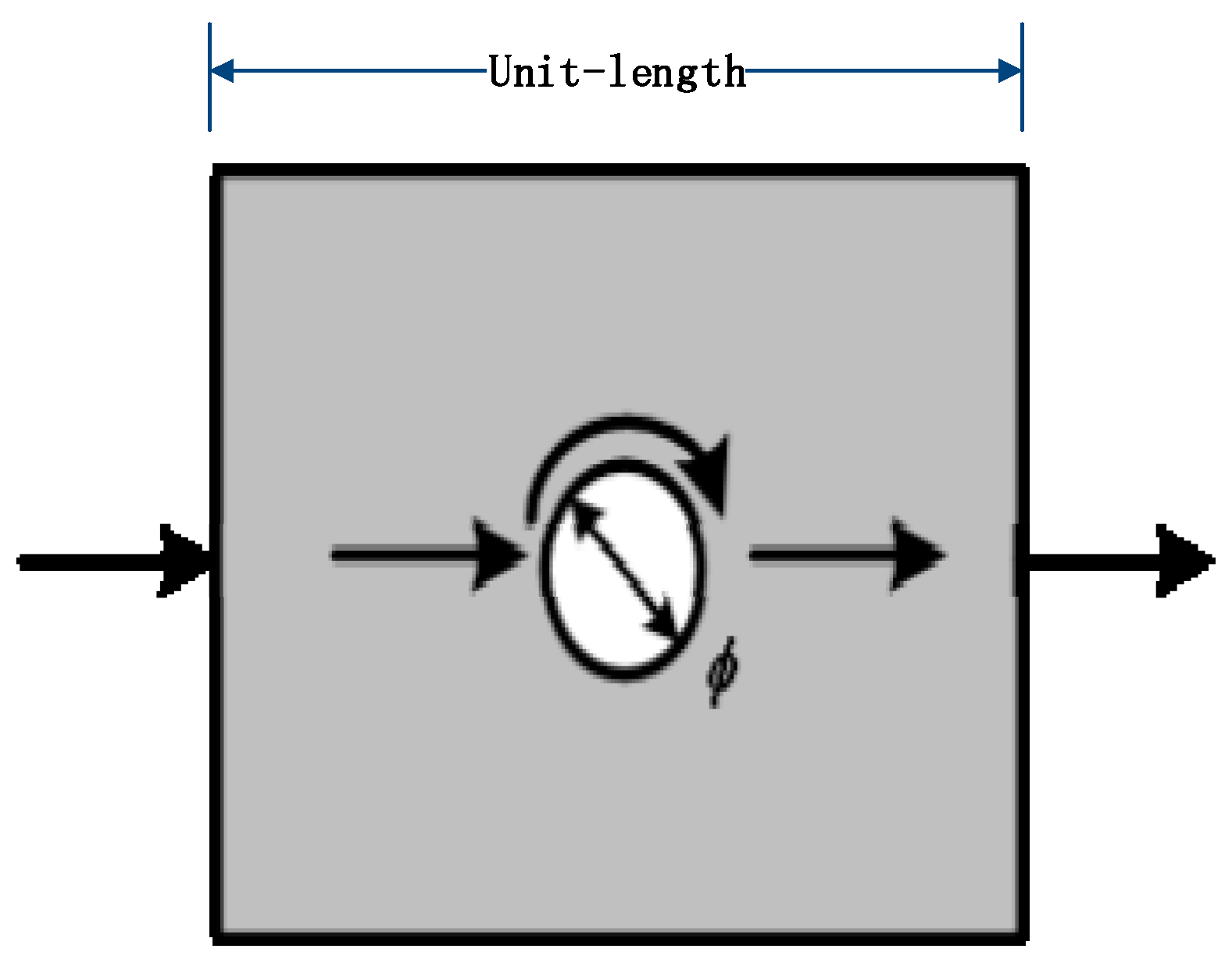
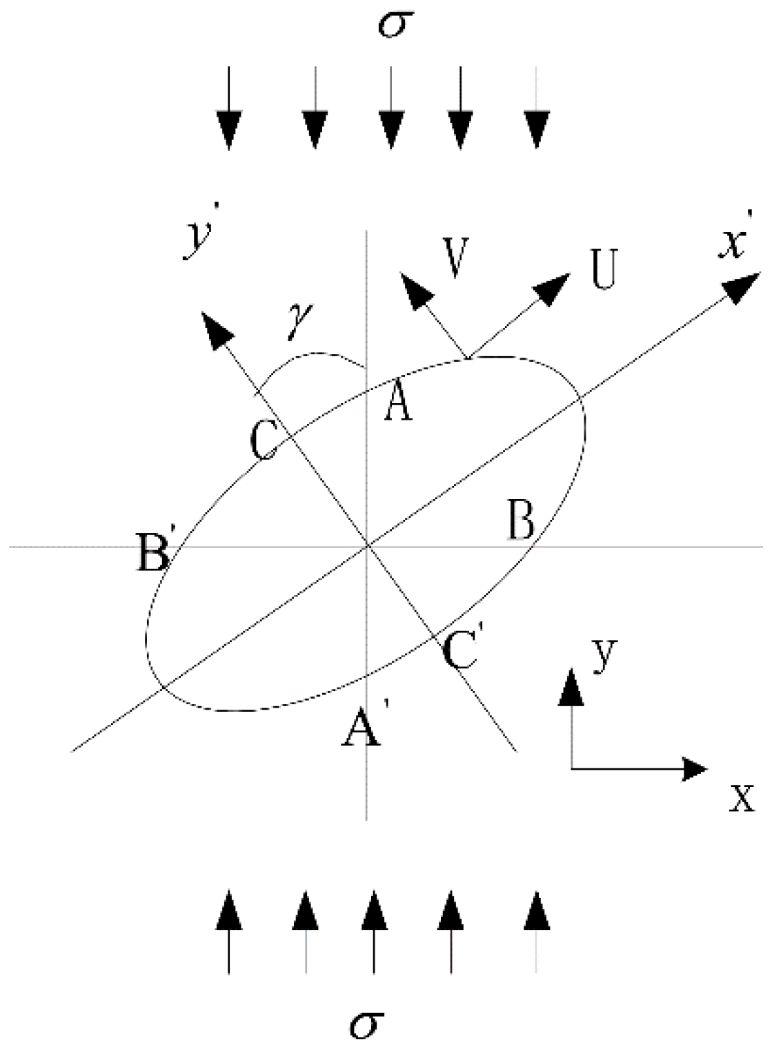
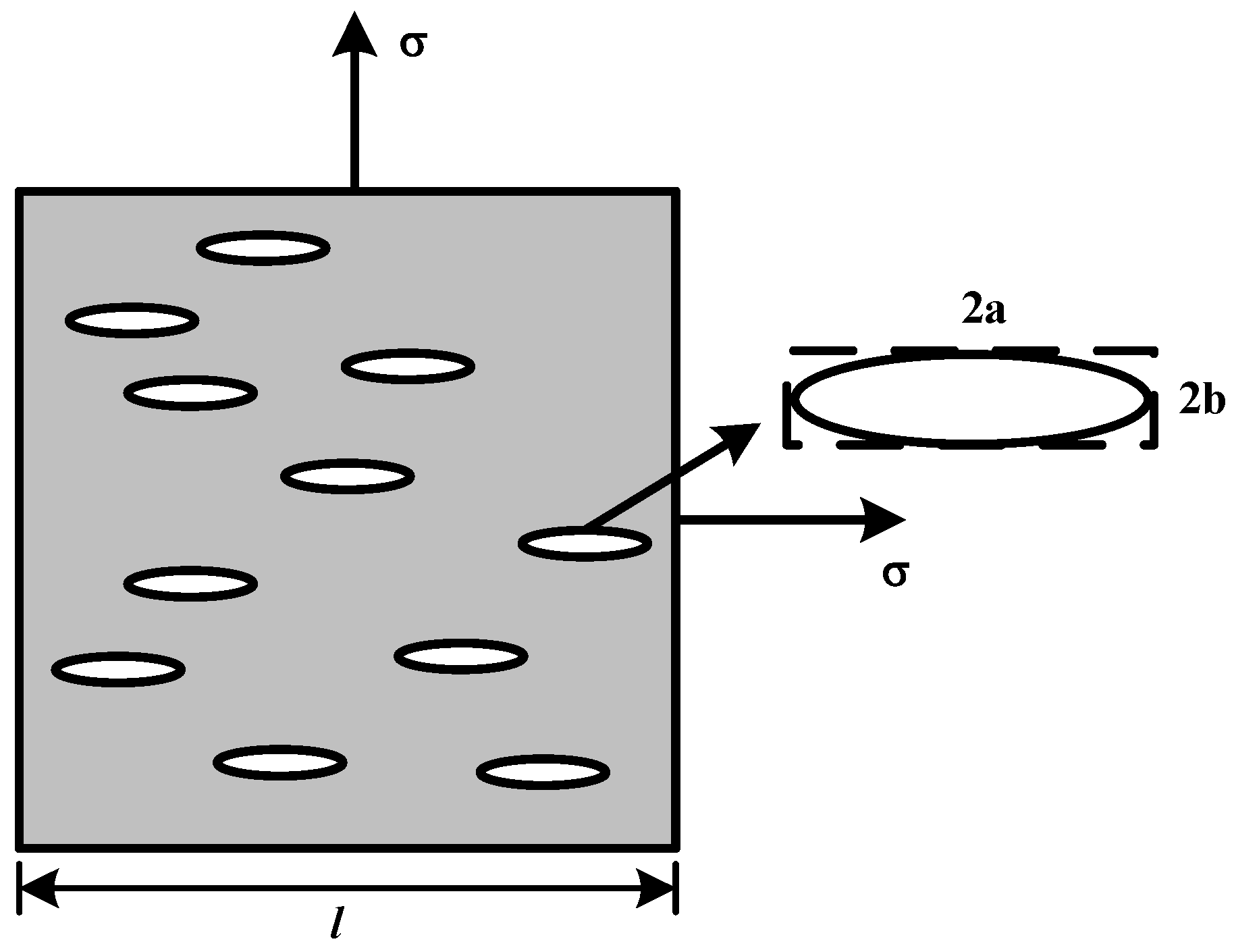
2.2. Crack Deformation under Uni-Axial Stress

The deformation of concrete under uni-axial stress is decomposed into the linear elastic deformation of the matrix, as well as the closed deformation and extended deformation of the microcracks. The axial strain and horizontal strain can be expressed as [23]:

$$\{\begin{array}{l}{\epsilon }_1\left(\sigma \right)={\epsilon }_1^{\mathrm{e}}+{\epsilon }_1^{\mathrm{c}}+{\epsilon }_1^{\mathrm{f}}\\ {\epsilon }_2\left(\sigma \right)={\epsilon }_2^{\mathrm{e}}+{\epsilon }_2^{\mathrm{c}}+{\epsilon }_2^{\mathrm{f}}\end{array}$$

(4)

where ${\epsilon }_i(\sigma )$ is the total deformation of the concrete; ${\epsilon }_i^{\mathrm{e}}$ is the deformation of the concrete matrix; ${\epsilon }_i^{\mathrm{c}}$ is the closed deformation of the microcracks; and ${\epsilon }_i^{\mathrm{f}}$ is the extended deformation of the microcracks. Here, i = 1, 2, … in which 1 and 2 represent the axial and horizontal directions, respectively.

The expressions of relative displacements of the cracks in the axial and horizontal directions can be derived based on the fracture mechanics theory. Suppose there is an elliptical crack in an infinite element loaded with a uniform compressive stress σ, as shown in Figure 2.

The displacement field around the crack can be expressed as shown in Equation (5):

$$\{\begin{array}{l}2G_{0}U=\frac{\sigma }{4}(k+1)b_0\cos \beta -\frac{\sigma }{4}(k+1)(a_0+b_0)\cos (2\gamma +\beta )\\ 2G_{0}V=\frac{\sigma }{4}(k+1)b_0\sin \beta -\frac{\sigma }{4}(k+1)(a_0+b_0)\sin (2\gamma +\beta )\end{array}$$

(5)

For the crack in Figure 1, the axial and horizontal displacements caused by the closure of the crack can be expressed by the relative displacement between points A-A’ and points B-B’. The displacement of points A and B caused by the stress σ can be expressed as shown in Equation (6).

$$\{\begin{array}{l}{U}_A^y=U_A\sin \gamma +V_A\cos \gamma =\frac{k+1}{8G_0}{a}_0(\sin \gamma \cos {\beta }_1+2\sin {\beta }_1\cos \gamma )\sigma \\ U_B^x=U_B\cos \gamma -V_B\sin \gamma =-\frac{k+1}{8G_0}{a}_0\cos {\beta }_2\cos \gamma \sigma \end{array}$$

(6)

Thus, the displacement caused by closure of the crack can be expressed as:

$$\{\begin{array}{l}{U}_1^y=\frac{k+1}{4G_0}{a}_0(\sin \gamma \cos {\beta }_1+2\sin {\beta }_1\cos \gamma )\sigma \\ U_2^x=\frac{k+1}{4G_0}{a}_0\cos {\beta }_2\cos \gamma \sigma \end{array}$$

(7)

Suppose the intensity of the crack in the element is k_N; then, the deformation of the element caused by stress σ can be calculated by Equation (8).

$$\{\begin{array}{l}{\epsilon }_1^{\mathrm{c}}=\frac{k+1}{2\pi G_0}{k}_{\mathrm{N}}{a}_0\sigma {\displaystyle {\int }_0^{\frac{\pi }{2}}(\sin \gamma \cos {\beta }_1+2\sin {\beta }_1\cos \gamma )\mathrm{d}\gamma }\\ {\epsilon }_2^{\mathrm{c}}=-\frac{k+1}{2\pi G_0}{k}_{\mathrm{N}}{a}_0\sigma {\displaystyle {\int }_0^{\frac{\pi }{2}}(\cos {\beta }_2\cos \gamma )\mathrm{d}\gamma }\end{array}$$

(8)

For the displacement caused by crack growth, the axial and horizontal displacements of a crack under stress σ can be expressed as:

$$\{\begin{array}{l}{U}_1^y=\frac{8\sqrt{2}T\tan \gamma }{\pi E_0}+\frac{32T^3}{{\pi }^2{K}_{Ic}^2{E}_0{a}_0\cos \gamma }\\ U_2^x=\frac{8\sqrt{2}T}{\pi E_0}-\frac{32T^3}{{\pi }^2{K}_{Ic}^2{E}_0{a}_0\sin \gamma }\end{array}$$

(9)

The deformation of the element induced by crack growth can be expressed as shown in Equation (10):

$$\{\begin{array}{l}{\epsilon }_1^{\mathrm{f}}=\frac{2}{\pi }{\displaystyle {\int }_0^{\frac{\pi }{2}}(\frac{8\sqrt{2}T{k}_{\mathrm{N}}\tan \gamma }{\pi E_0}+\frac{32T^3{k}_{\mathrm{N}}}{{\pi }^2{K}_{Ic}^2{E}_0{a}_0\cos \gamma })\mathrm{d}\gamma }\\ {\epsilon }_2^{\mathrm{f}}=-\frac{2}{\pi }{\displaystyle {\int }_0^{\frac{\pi }{2}}(\frac{8\sqrt{2}T{k}_{\mathrm{N}}}{\pi E_0}+\frac{32T^3{k}_{\mathrm{N}}}{{\pi }^2{K}_{\mathrm{Ic}}^2{E}_0{a}_0\sin \gamma })\mathrm{d}\gamma }\end{array}$$

(10)

where $E_0$, $k$, $G_0$ are the elastic constants of the concrete; $K_{\mathrm{IC}}$ is the fracture toughness of the concrete, $k_{\mathrm{N}}$ is the crack density parameter in unit volume concrete; $a_0$ is the semi-major axis of the concrete microcrack, which is determined by the shape of the crack; $\gamma$ and ${\beta }_1$ are the orientation parameter of the crack; and $T$ is proportional to the stress $\sigma -{\sigma }_u$, in which ${\sigma }_u$ is the critical stress of the crack closure or expansion.

Because the micro-parameters of concrete material are not easily determined in practice, Equations (8) and (10) need to be further simplified. If the elastic properties of the concrete elastic matrix are constant under stress, from Equations (8) and (10), it can be seen that the closure deformation of the crack is only proportional to the $\sigma$, and the expansion deformation depends on the ${(\sigma -{\sigma }_{\mathrm{u}})}^3$ and $(\sigma -{\sigma }_{\mathrm{u}})$.

Then, the volume strain of the crack closure can be simplified as:

$${\epsilon }_{\mathrm{V}}^{\mathrm{c}}={\epsilon }_1^{\mathrm{c}}+2{\epsilon }_2^{\mathrm{c}}=k_{\mathrm{a}}\sigma$$

(11)

Furthermore, the volume strain of the crack expansion can be simplified as:

$${\epsilon }_{\mathrm{V}}^{\mathrm{f}}={\epsilon }_1^{\mathrm{f}}+2{\epsilon }_2^{\mathrm{f}}=k_{\mathrm{b}1}(\sigma -{\sigma }_{\mathrm{u}})+k_{\mathrm{b}2}{(\sigma -{\sigma }_{\mathrm{u}})}^3$$

(12)

where k_a, k_b1, and k_b2 are undetermined coefficients.

2.3. Sound Velocity Change Induced by Uni-Axial Stress

By analyzing the deformation of a crack under uni-axial stress, it is found that the axial closure deformation of the crack is much more than the horizontal deformation. At the same time, the secondary cracks in the extended stage are along the axial direction. Then the acoustoelastic properties of concrete can be described as follows: the sound velocity change caused by the closure volume deformation of the primary microcracks is equivalent to that caused by a set of horizontal cracks, and the sound velocity change caused by the extended volume deformation of the microcracks is equivalent to that caused by a set of vertical cracks. Moreover, the equivalent cracks have the same properties as the original cracks. It should be noted that the concrete cracks described here are equivalent cracks and the deformation of concrete cracks is not analyzed from the viewpoint of the microscopic mechanism.

If the density parameter of the horizontal equivalent cracks in the concrete is $x_1$, it can be approximately expressed as follows:

$$x_1=k_{\mathrm{N}}\frac{{\epsilon }_{\mathrm{V}}^{\mathrm{c}}}{\varphi }$$

(13)

where $k_{\mathrm{N}}$ represents the crack density of the concrete without loading.

In the same way, the density parameter of the extended equivalent cracks $x_2$ can be expressed as follows:

$$x_2=k_{\mathrm{N}}\frac{{\epsilon }_{\mathrm{V}}^{\mathrm{f}}}{\varphi }$$

(14)

Set a group of horizontal opening oval cracks in the concrete element with length l. The long- and short-axes of the crack are denoted as 2a and 2b, respectively, as shown in Figure 3. Without considering the evolution of microcracks, for the convenience of modeling, we simplified the microcrack shape as a rectangular with a size of 2a × 2b.

Suppose the sound wave passes through the concrete element with equal probability density. If the sound wave encounters cracks, it will bypass the cracks and propagation along the boundary of the concrete matrix. When the sound wave passes through the element from the direction perpendicular to the long-axis direction of the crack, the probability of passing through a microcrack is $\frac{2a}{l}$. At this time, the average propagation path length of the sound wave is $l+2a$, the probability of not passing through the crack is $\frac{l-2a}{l}$, and the average propagation path length of the sound wave is $l$. Then, the increment of the acoustic slowness caused by microcracks is:

$$\Delta S_1=S_1-S_{pm}=\frac{\frac{2a}{l}\frac{l+2a}{V_{pm}}+\frac{l-2a}{l}\frac{l}{V_{pm}}}{l}-S_{pm}=\frac{4a^2}{l^2}{S}_{pm}$$

(15)

where S₁ denotes the acoustic slowness caused by the microcrack when the sound wave passes through the element in the short-axis direction of the crack.

In the same way, when the sound wave passes through the element in the direction parallel to the long-axis of that crack, the increment of the acoustic slowness caused by the microcrack can be expressed as:

$$\Delta S_2=\frac{4b^2}{l^2}{S}_{\mathrm{pm}}$$

(16)

By introducing $k_{\alpha }$ to represent the shape correction coefficient of an elliptical crack in a rectangular crack, and substituting Equations (13) and (14) into Equations (15) and (16), respectively, we can obtain increments of the acoustic slowness in the axial and the horizontal directions due to the crack closure or expansion deformation, as shown in Equation (17).

$$\{\begin{array}{l}\Delta S_{\mathrm{p},1}^{\mathrm{c}}=4k_{\mathsf{\alpha }}{x}_1{a}_0^2{S}_{\mathrm{pm}}=4k_{\mathsf{\alpha }}{k}_{\mathrm{N}}\frac{{\epsilon }_{\mathrm{V}}^{\mathrm{c}}}{\varphi }{a}_0^2{S}_{\mathrm{pm}}=4k_{\mathsf{\alpha }}{k}_{\mathrm{N}}\frac{k_{\mathrm{a}}\sigma }{\varphi }{a}_0^2{S}_{\mathrm{pm}}\\ \Delta S_{\mathrm{p},1}^{\mathrm{f}}=4k_{\mathsf{\alpha }}{x}_2{b}_0^2{S}_{\mathrm{pm}}=4k_{\mathsf{\alpha }}{k}_{\mathrm{N}}\frac{{\epsilon }_{\mathrm{V}}^{\mathrm{f}}}{\varphi }{b}_0^2{S}_{\mathrm{pm}}=4k_{\mathsf{\alpha }}{k}_{\mathrm{N}}\frac{k_{\mathrm{b}1}(\sigma -{\sigma }_{\mathrm{u}})+k_{\mathrm{b}2}{(\sigma -{\sigma }_{\mathrm{u}})}^3}{\varphi }{b}_0^2{S}_{\mathrm{pm}}\\ \Delta S_{\mathrm{p},\mathrm{2}}^{\mathrm{c}}=4k_{\mathsf{\alpha }}{x}_1{b}_0^2{S}_{\mathrm{pm}}=4k_{\mathsf{\alpha }}{k}_{\mathrm{N}}\frac{{\epsilon }_V^c}{\varphi }{b}_0^2{S}_{\mathrm{pm}}=4k_{\mathsf{\alpha }}{k}_{\mathrm{N}}\frac{k_{\mathrm{a}}\sigma }{\varphi }{b}_0^2{S}_{\mathrm{pm}}\\ \Delta S_{\mathrm{p},\mathrm{2}}^{\mathrm{f}}=4k_{\mathsf{\alpha }}{x}_2{a}_0^2{S}_{\mathrm{pm}}=4k_{\mathsf{\alpha }}{k}_{\mathrm{N}}\frac{{\epsilon }_{\mathrm{V}}^{\mathrm{f}}}{\varphi }{a}_0^2{S}_{\mathrm{pm}}=4k_{\mathsf{\alpha }}{k}_{\mathrm{N}}\frac{k_{\mathrm{b}1}(\sigma -{\sigma }_{\mathrm{u}})+k_{\mathrm{b}2}{(\sigma -{\sigma }_{\mathrm{u}})}^3}{\varphi }{a}_0^2{S}_{\mathrm{pm}}\end{array}$$

(17)

where $\Delta S_{\mathrm{p},1}^{\mathrm{c}}$, $\Delta S_{\mathrm{p},1}^{\mathrm{f}}$, $\Delta S_{\mathrm{p},2}^{\mathrm{c}}$, and $\Delta S_{\mathrm{p},2}^{\mathrm{f}}$ represent the increment of the acoustic slowness caused by the crack closure and expansion in the axial and horizontal directions, respectively.

According to Equation (3), Equation (18) is rewritten into the form of a slowness ratio.

$$\{\begin{array}{l}\frac{\Delta S_{\mathrm{p}1}^{\mathrm{c}}}{S_{p0}}=\frac{4k_{\mathsf{\alpha }}{k}_{\mathrm{N}}\frac{k_{\mathrm{a}}\sigma }{\varphi }{a}_0^2{S}_{\mathrm{pm}}}{(1+0.57\varphi )S_{\mathrm{pm}}}=\frac{4k_{\mathsf{\alpha }}{k}_{\mathrm{N}}}{\varphi (1+0.57\varphi )}{a}_0^2{k}_{\mathrm{a}}\sigma \\ \frac{\Delta S_{\mathrm{p}1}^f}{S_{p0}}=\frac{4k_{\mathsf{\alpha }}{k}_{\mathrm{N}}\frac{k_{\mathrm{b}1}(\sigma -{\sigma }_{\mathrm{u}})+k_{\mathrm{b}2}{(\sigma -{\sigma }_{\mathrm{u}})}^3}{\varphi }{b}_0^2{S}_{\mathrm{pm}}}{(1+0.57\varphi )S_{\mathrm{pm}}}=\frac{4k_{\mathsf{\alpha }}{k}_{\mathrm{N}}}{\varphi (1+0.57\varphi )}{b}_0^2[k_{\mathrm{b}1}(\sigma -{\sigma }_{\mathrm{u}})+k_{\mathrm{b}2}{(\sigma -{\sigma }_{\mathrm{u}})}^3]\\ \frac{\Delta S_{\mathrm{p}2}^{\mathrm{c}}}{S_{p0}}=\frac{4k_{\mathsf{\alpha }}{k}_{\mathrm{N}}\frac{k_{\mathrm{a}}\sigma }{\varphi }{b}_0^2{S}_{\mathrm{pm}}}{(1+0.57\varphi )S_{\mathrm{pm}}}=\frac{4k_{\mathsf{\alpha }}{k}_{\mathrm{N}}}{\varphi (1+0.57\varphi )}{b}_0^2{k}_{\mathrm{a}}\sigma \\ \frac{\Delta S_{\mathrm{p}2}^f}{S_{p0}}=\frac{4k_{\mathsf{\alpha }}{k}_{\mathrm{N}}\frac{k_{\mathrm{b}1}(\sigma -{\sigma }_{\mathrm{u}})+k_{\mathrm{b}2}{(\sigma -{\sigma }_{\mathrm{u}})}^3}{\varphi }{a}_0^2{S}_{\mathrm{pm}}}{(1+0.57\varphi )S_{\mathrm{pm}}}=\frac{4k_{\mathsf{\alpha }}{k}_{\mathrm{N}}}{\varphi (1+0.57\varphi )}{a}_0^2[k_{\mathrm{b}1}(\sigma -{\sigma }_{\mathrm{u}})+k_{\mathrm{b}2}{(\sigma -{\sigma }_{\mathrm{u}})}^3]\end{array}$$

(18)

Defining k_s as parameter related to the shape and density of crack, $k_{\mathrm{s}}=4k_{\mathsf{\alpha }}{k}_{\mathrm{N}}\frac{a_0^2}{\varphi (1+1.57\varphi )}$, Equation (18) can be simplified as:

$$\{\begin{array}{l}\frac{\Delta S_{\mathrm{p},1}^{\mathrm{c}}}{S_{\mathrm{p}0}}=k_{\mathrm{s}}{k}_{\mathrm{a}}\sigma \\ \frac{\Delta S_{\mathrm{p},1}^{\mathrm{f}}}{S_{\mathrm{p}0}}=k_{\mathrm{s}}{\left(\frac{b_0}{a_0}\right)}^2[k_{\mathrm{b}1}(\sigma -{\sigma }_{\mathrm{u}})+k_{\mathrm{b}2}{(\sigma -{\sigma }_{\mathrm{u}})}^3]\\ \frac{\Delta S_{\mathrm{p},2}^{\mathrm{c}}}{S_{\mathrm{p}0}}=k_{\mathrm{s}}{\left(\frac{b_0}{a_0}\right)}^2{k}_{\mathrm{a}}\sigma \\ \frac{\Delta S_{\mathrm{p},1}^{\mathrm{f}}}{S_{\mathrm{p}0}}=k_{\mathrm{s}}[k_{\mathrm{b}1}(\sigma -{\sigma }_{\mathrm{u}})+k_{\mathrm{b}2}{(\sigma -{\sigma }_{\mathrm{u}})}^3]\end{array}$$

(19)

Let $k_{\mathrm{c}1}=k_{\mathrm{s}}{k}_{\mathrm{a}}$, $k_{\mathrm{f}1}={\alpha }^2{k}_{\mathrm{s}}{k}_{\mathrm{b}1}$, $k_{\mathrm{f}2}={\alpha }^2{k}_{\mathrm{s}}{k}_{\mathrm{b}2}$, $k_{\mathrm{c}2}={\alpha }^2{k}_{\mathrm{s}}{k}_{\mathrm{a}}$, $k_{\mathrm{f}21}=k_{\mathrm{s}}{k}_{\mathrm{b}1}$, and $k_{\mathrm{f}22}=k_{\mathrm{s}}{k}_{\mathrm{b}2}$. These parameters are only related to the crack, but not related to stress.

Then, the axial and horizontal relative acoustic slowness of the sound wave propagating in the concrete can be obtained as:

Axial relative acoustic slowness in the crack closure stage:

$$\frac{\Delta S_1}{S_{\mathrm{p}0}}=-k_{\mathrm{c}1}\sigma$$

(20a)

Axial relative acoustic slowness in the crack expansion stage:

$$\frac{\Delta S_1}{S_{\mathrm{p}0}}=-\frac{\Delta S_{\mathrm{p},1}^c}{S_{\mathrm{p}0}}+\frac{\Delta S_{\mathrm{p},1}^{\mathrm{f}}}{S_{\mathrm{p}0}}=-k_{\mathrm{c}1}{\sigma }_{\mathrm{u}}+k_{\mathrm{f}11}(\sigma -{\sigma }_{\mathrm{u}})+k_{\mathrm{f}12}{(\sigma -{\sigma }_{\mathrm{u}})}^3$$

(20b)

Horizontal relative acoustic slowness in the crack closure stage:

$$\frac{\Delta S_2}{S_{\mathrm{p}0}}=-k_{\mathrm{c}2}\sigma$$

(20c)

Horizontal relative acoustic slowness in the crack expansion stage:

$$\frac{\Delta S_2}{S_{\mathrm{p}0}}=-\frac{\Delta S_{p,2}^c}{S_{\mathrm{p}0}}+\frac{\Delta S_{p,2}^f}{S_{\mathrm{p}0}}=-k_{\mathrm{c}2}{\sigma }_{\mathrm{u}}+k_{\mathrm{f}21}(\sigma -{\sigma }_{\mathrm{u}})+k_{\mathrm{f}22}{(\sigma -{\sigma }_{\mathrm{u}})}^3$$

(20d)

Because the acoustic slowness and sound velocity are reciprocal, it is easy to obtain the following relation:

$$(1+\frac{\Delta S_i}{S_{\mathrm{p}0}})(1+\frac{\Delta V_i}{V_{\mathrm{p}0}})=1\hspace{1em}\hspace{1em}(i=1,2)$$

(21)

Changing the acoustic slowness to the sound velocity, we can then obtain the following.

Axial relative sound velocity in the crack closed stage:

$$\frac{\Delta V_1}{V_{\mathrm{p}0}}=\frac{1}{1-k_{\mathrm{c}1}\sigma }-1$$

(22a)

Axial relative sound velocity in the crack extended stage:

$$\frac{\Delta V_1}{V_{\mathrm{p}0}}=\frac{1}{1-k_{\mathrm{c}1}{\sigma }_{\mathrm{u}}+k_{\mathrm{f}11}(\sigma -{\sigma }_{\mathrm{u}})+k_{\mathrm{f}12}{(\sigma -{\sigma }_{\mathrm{u}})}^3}-1$$

(22b)

Horizontal relative sound velocity in the crack closed stage:

$$\frac{\Delta V_2}{V_{\mathrm{p}0}}=\frac{1}{1-k_{\mathrm{c}2}\sigma }-1$$

(22c)

Horizontal relative sound velocity in the crack extended stage:

$$\frac{\Delta V_2}{V_{\mathrm{p}0}}=\frac{1}{1-k_{\mathrm{c}2}{\sigma }_{\mathrm{u}}+k_{\mathrm{f}21}(\sigma -{\sigma }_{\mathrm{u}})+k_{\mathrm{f}22}{(\sigma -{\sigma }_{\mathrm{u}})}^3}-1$$

(22d)

3. Experimental Investigation

In order to verify the rationality of the model, an experiment of CWI under stress in concrete was carried out. The propagating law of the coda wave in concrete was first investigated, and then the relation between the wave velocity and stress was calibrated by step loading. The experiment was conducted using a pulse generator to transmit a pulse signal, which can excite the transmission energy converter, causing it to vibrate, and generate an ultrasonic signal to pass through the test specimens. Finally, sensors received the signal and the data were recorded by a data collector.

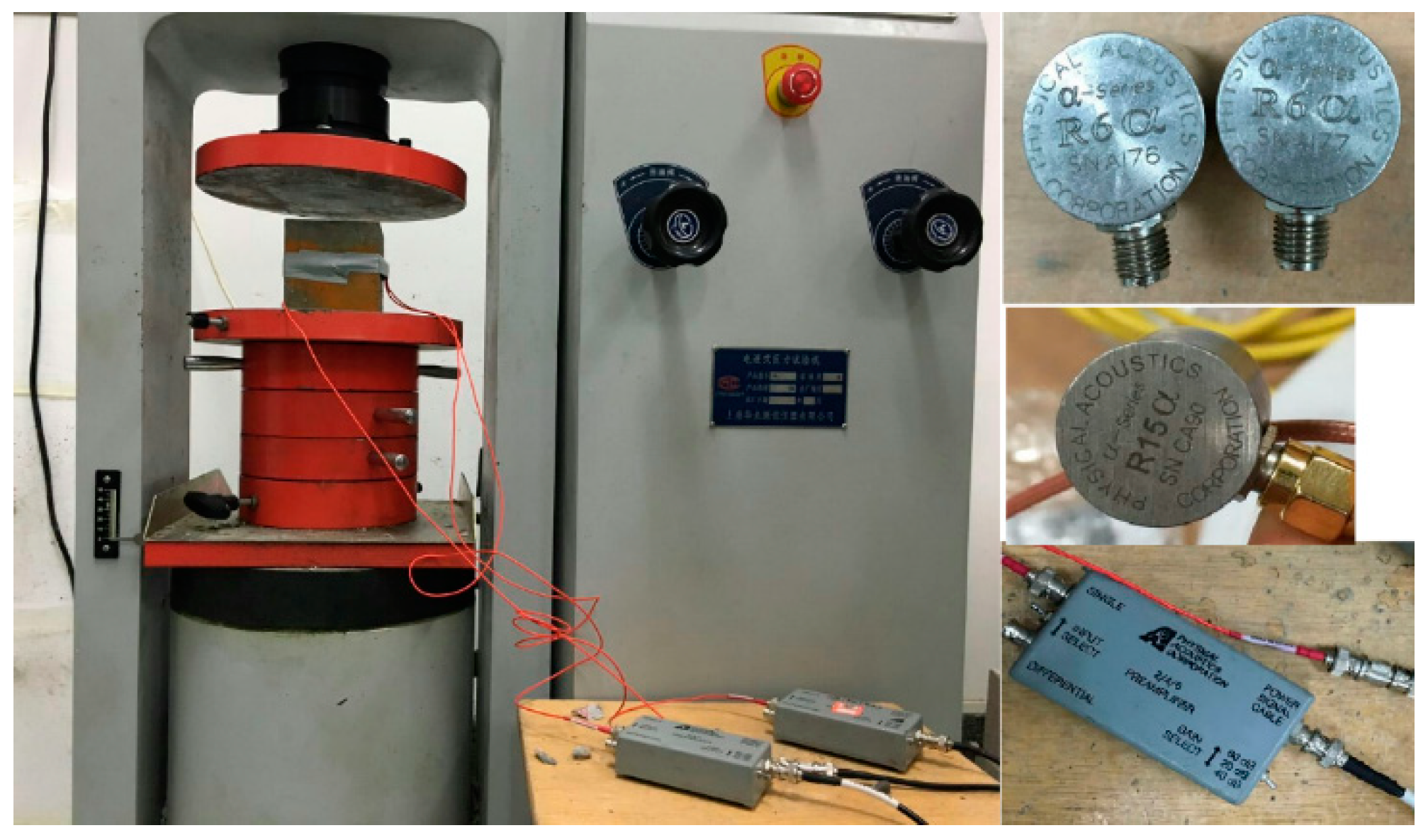
3.1. Experimental System and Sensors

The experimental system was mainly composed of a pulse generator, transmitter and receiver, data acquisition system, and an electro-hydraulic pressure testing machine. The signal generator used in the experiment was a 14-bit digital-to-analog conversion signal card, which can generate 100 M sample points of the ultrasound signal. The output signal of the pulse generator was 10 volts and the frequency ranged up to 15 MHz. A resonant piezoelectric ceramic transducer was selected to be the sensor for the wave’s transmitter and receiver. In this experiment, three kinds of sensors with frequencies of 300 kHz, 150 kHz, and 50 kHz were used, the specific parameters of which are listed in

Table 1. Performance parameters of sensors.

Center Frequency (kHz)	Size (mm)	Weight (g)	Operating Temperature Range (°C)	Frequency Range (kHz)	Resonance Frequency (kHz)
300	8 × 8	2	−65~177	150~400	300
150	23 × 19	27	−45~125	50~200	150
50	23 × 19	33	−45~125	35~80	50

. A signal amplifier was used in the experiment to guarantee that the received signal could be identified. A 40 db–60 db transmission gain could be supported by the amplifier. The sampling rate of the data acquisition system was set as 40 MHz and the maximum length of a single data signal could be recorded at 15 kB. The time interval to record each test point was 1 s. About 100 waveforms were recorded in the experiment, and the signal to noise ratio was improved by the superposition. During the experiment, the temperature and humidity of the environment were strictly monitored and controlled to eliminate their effects on the test results. An electro-hydraulic pressure testing machine was adopted in the experiment to provide compression on the specimen to analyze the influence of stress in concrete on the coda waves. The equipment is shown in Figure 4.

3.2. Specimen Arrangement

Concrete specimens were cubes with a size of 100 mm × 100 mm × 100 mm, and their mixture proportions are listed in

Table 2. Concrete mix ratio parameter.

Composition	Cement	Sand	Aggregate	Water	Admixture
Dosage per m3 (kg)	420	622	1155	210	2.10 (1%)

. The specimens were divided into four groups, respectively coded as A, B, C-1, and C-2. Group A was used to test the development of the coda wave in concrete, Group B was used to determine the strength of the concrete, and Group C was used for stress velocity calibration (C-1 for the calibration of axial velocity, and the C-2 for the calibration of horizontal velocity).

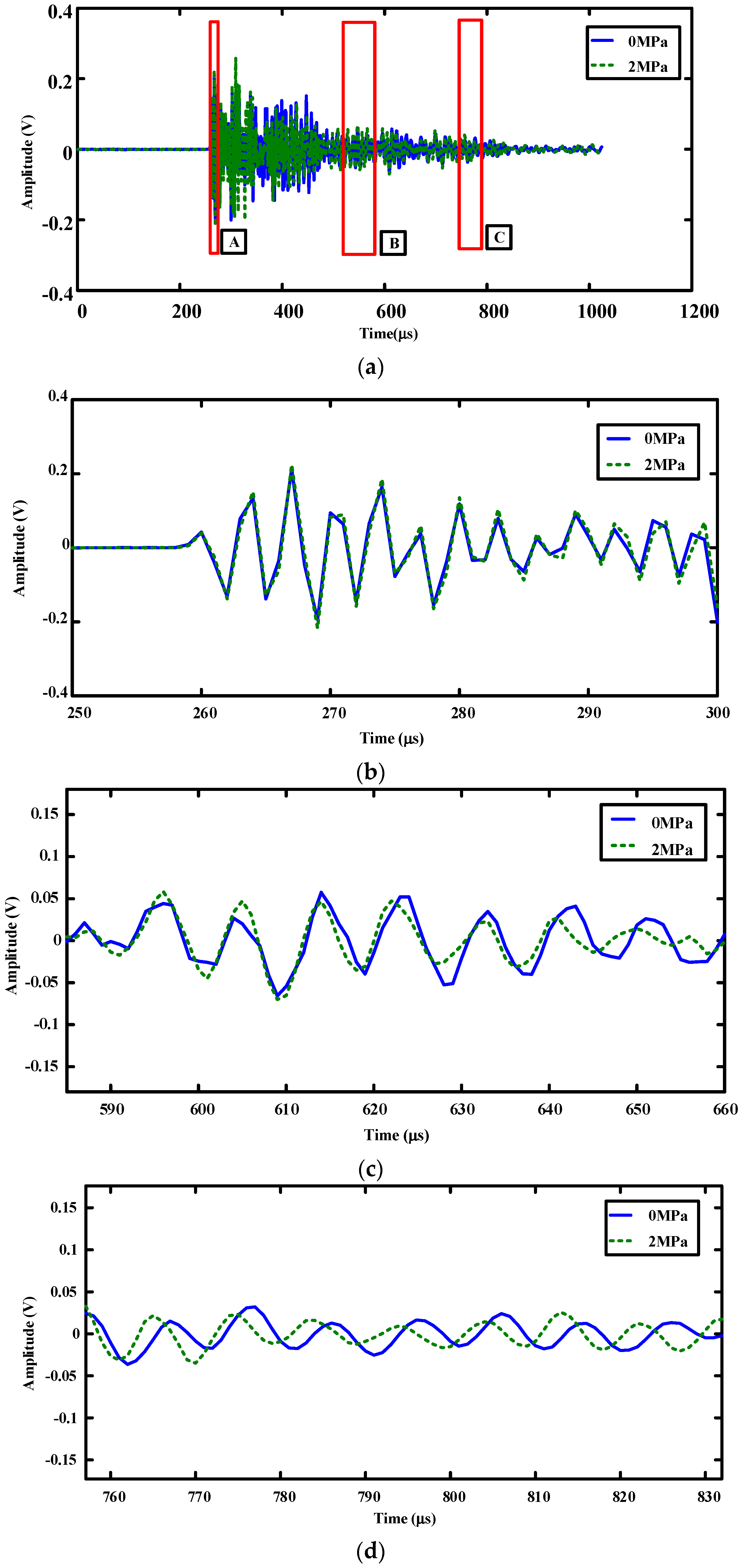
3.3. Propagating Regularity of the Coda Wave in Concrete

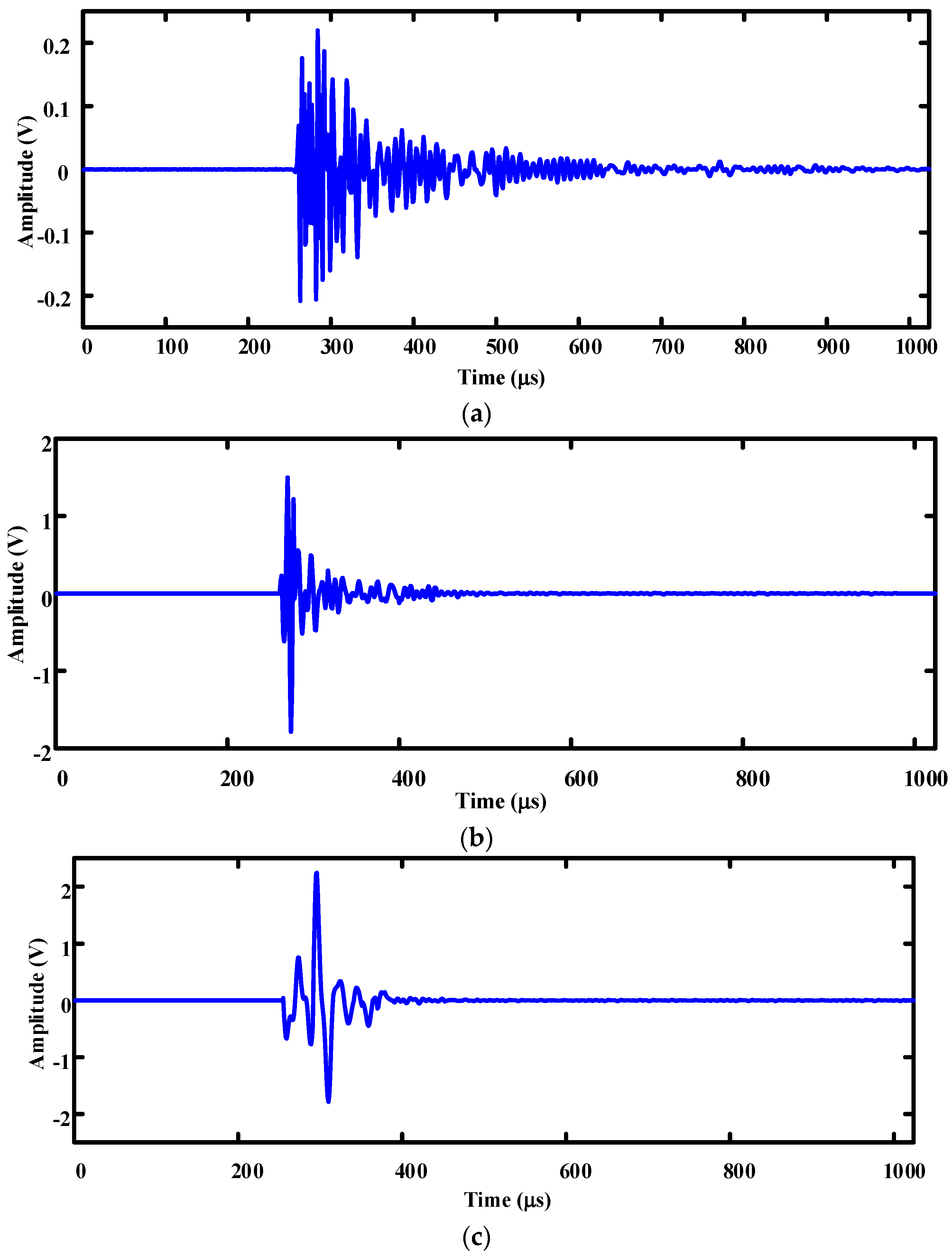
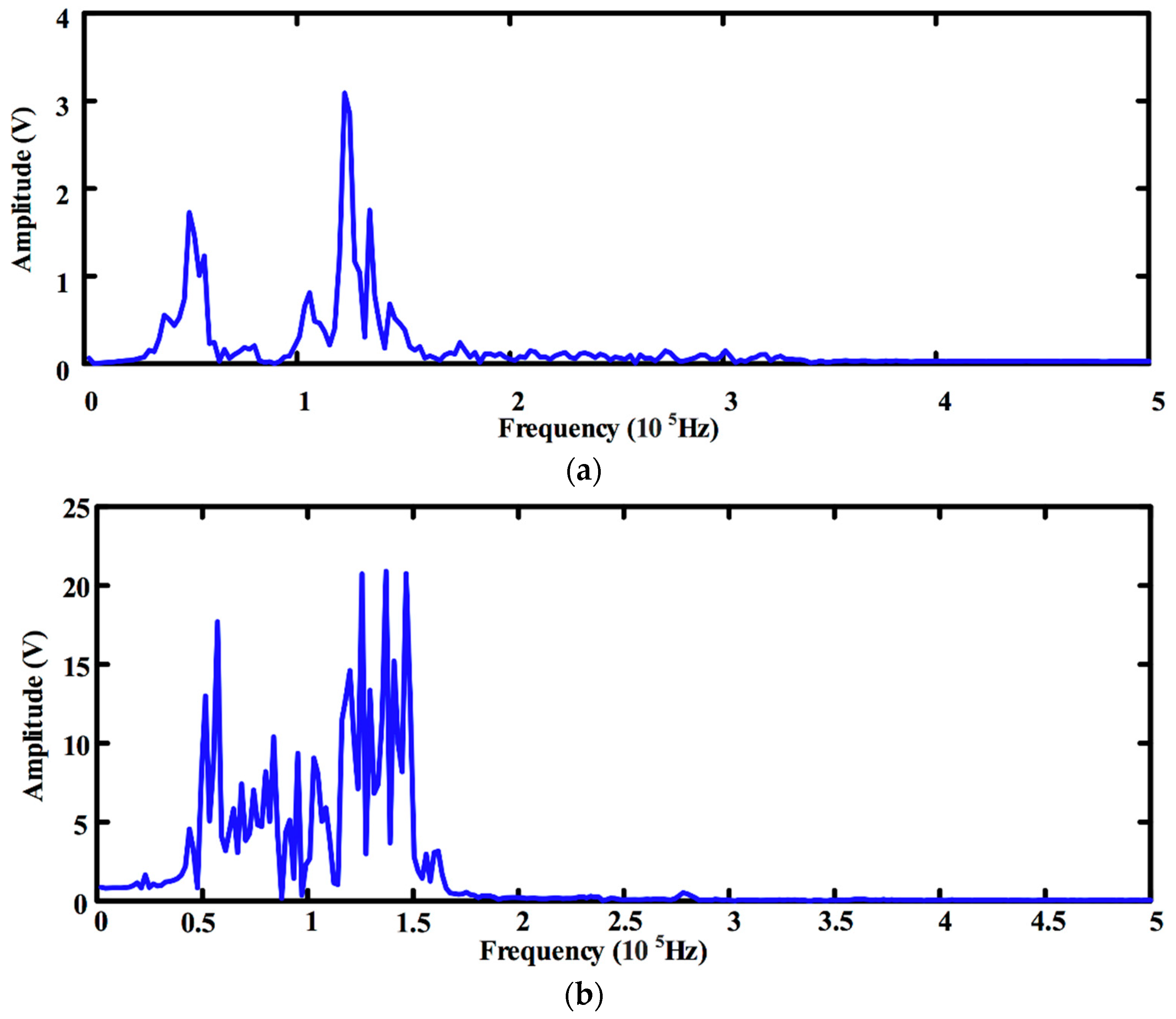
3.3.1. Frequency Effect

Figure 5 depicts the waveforms at transmission signal frequencies of 300 kHz, 150 kHz, and 50 kHz. It was found from the received waveforms of three different frequencies that the attenuation of the first wave amplitude with a frequency of 300 kHz is about 2%. The first wave amplitudes with frequencies of 50 kHz and 150 kHz also have certain levels attenuation, but they are much smaller than that at 300 kHz. This is because the wavelength of the high-frequency sound wave is shorter than the size of aggregates and defects, resulting in more refracted and scattered wave. So, a large part of the energy is reflected back or scattered around these obstacles. This indicates that a high-frequency wave has an unavoidable defect when used in concrete testing by the direct wave method, due to its rapid attenuation. However, as shown in Figure 4a, coda waves at 300 kHz developed well, manifesting a larger amplitude and longer duration than those at 150 kHz in Figure 4b and 50 kHz in Figure 4c. When a wavelength is close to the size of the obstacles it encounters, multiple scattering occurs, and a coda wave will form. This demonstrates that the higher the frequency is, the better the coda waves develop. As shown in Figure 4c, the coda wave at 50 kHz is basically not developed, so an acoustic wave with this frequency is not suitable for the CWI test.

Coda wave spectrums of acoustic signals at 300 kHz and 150 kHz are shown in Figure 6. It was found that the main frequency of the coda wave tends to move towards the low-frequency direction. The spectrum drift of the acoustic signal with a main frequency of 300 kHz is the most obvious. Its coda wave frequency is concentrated in the vicinity of 50 kHz and 130 kHz, while the coda wave frequency of the acoustic signal of 150 kHz is concentrated in the range of 50 kHz to 150 kHz. This is because the coda wave is formed by multiple scattering, and the interaction of the various acoustic interfaces in the concrete causes the wavelength of the acoustic signal to become longer and the frequency to become lower.

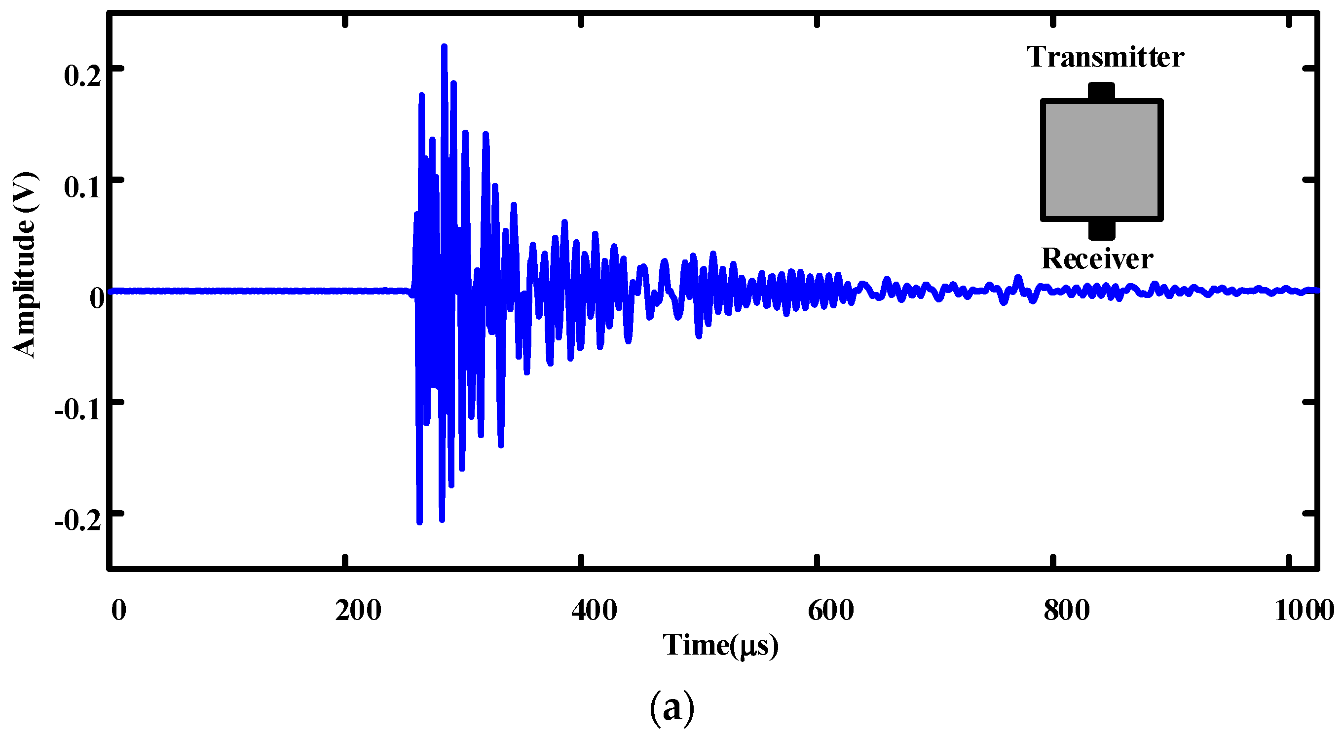
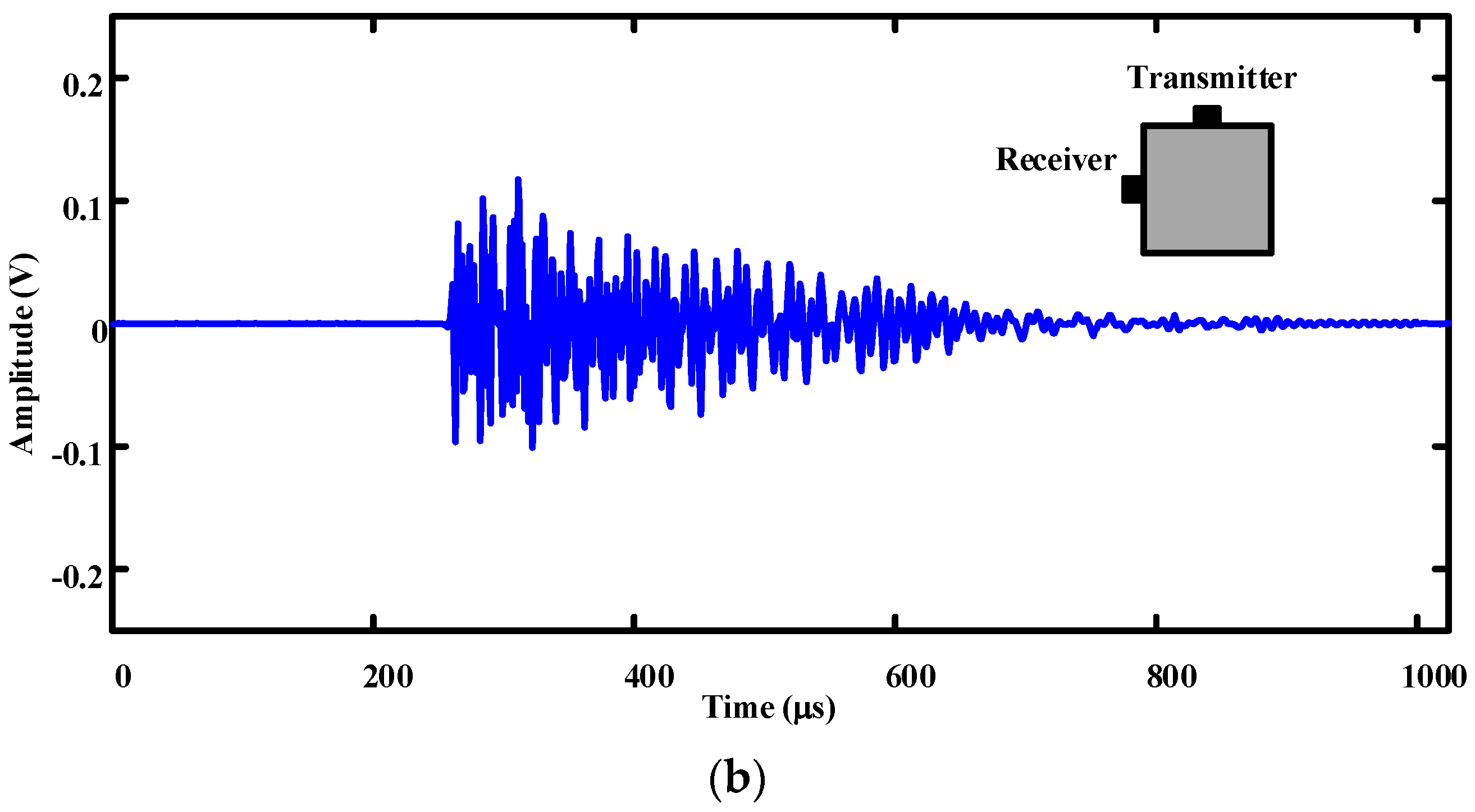
3.3.2. Influence of the Relative Position of Transmitters and Receivers

Waveforms of the receivers set on the opposite side and top of the transmitter are shown in Figure 7. It was found that the coda wave of an acoustic signal launched from the top surface and received on the side is more developed than that launched and received on the opposite surface. The main reasons for this are listed as follows. Firstly, the received signal launched on the top surface and received on the side is an example of non-collinear propagation. In the process of propagation, the direct wave cannot be perceived. Secondly, the waveform launched on the top surface and received on the side contains a certain component of transverse wave due to the different wave field. There is a large angle between the polarization direction and propagation direction of the transverse wave, but the polarization direction of the longitudinal wave is the same as the propagation direction. Therefore, the scattering probability of the transverse wave is larger, the scattering energy is strong, and the coda wave is more developed.

3.4. The Coda Wave Test under Uni-Axial Stress

3.4.1. CWI Analysis Method

The CWI method is employed to measure the change of the wave velocity based on the correlation of the waveforms before and after the disturbance. Define the initial waveform as $u(t)$. After the disturbance, the waveform transfers to $u[t(1-\epsilon )]$. Then, the correlation function can be expressed as [24]:

$$C(\epsilon )=\frac{{\displaystyle \int u[t(1-\epsilon )]u(t)\mathrm{d}t}}{\sqrt{{\displaystyle \int u^2[t(1-\epsilon )]dt{\displaystyle \int u^2(t)\mathrm{d}t}}}}$$

(23)

If $C(\epsilon )$ reaches the maximum value, then:

$${\epsilon }_k=-\frac{\delta v}{v}$$

(24)

The wave source of CWI must have high repeatability. Figure 8a depicts the receiving signal waveforms when the specimens are loaded with 0 MPa and 2 MPa. To clearly present the difference between the two waveforms, three time windows were enlarged, and they are shown in Figure 8b–d. A, B, and C represent the three windows of the waveform at different times, which enables an investigation of the development of two kinds of loading condition in different time windows. The later the time, the more complete the coda wave development. From Figure 8b, it was found that the time window A of both basically coincide with each other and no detectable changes occur, which ensures the repeatability of the experiment. As shown in Figure 8c, the time window B exhibits a certain phase deviation. In the time window C, however, there is a more obvious phase deviation, as shown in Figure 8d. This indicates that stress in concrete (<10 MPa) would make the concrete denser, resulting in a higher elastic modulus of the concrete and a higher velocity of the acoustic wave. It can be also concluded that the coda wave is sensitive to slight changes in the medium.

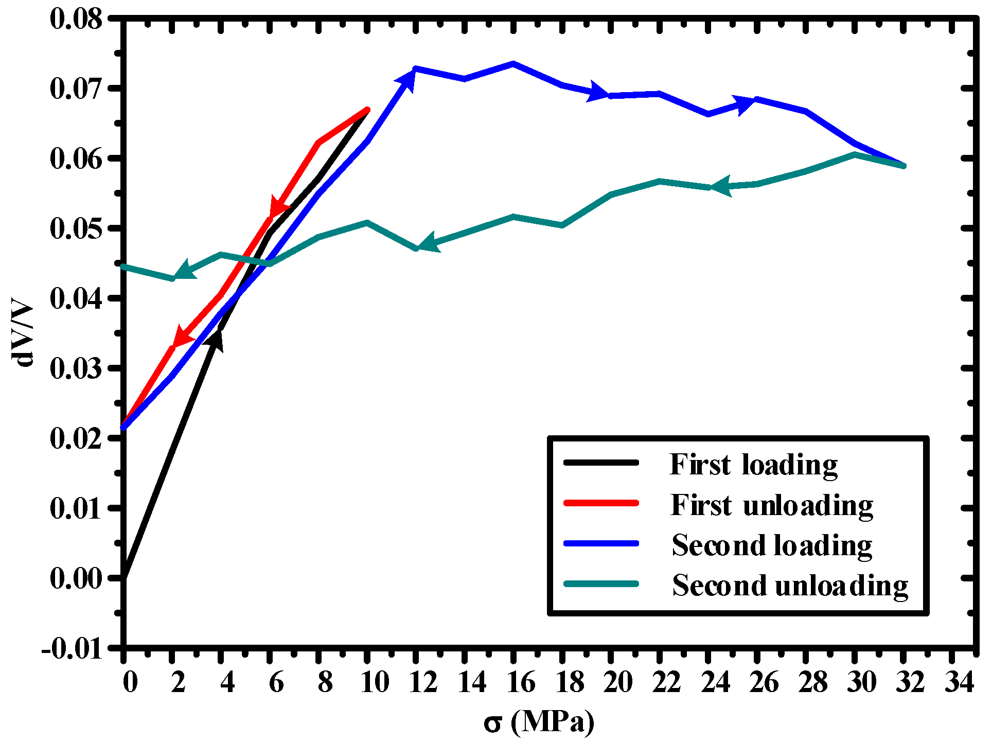
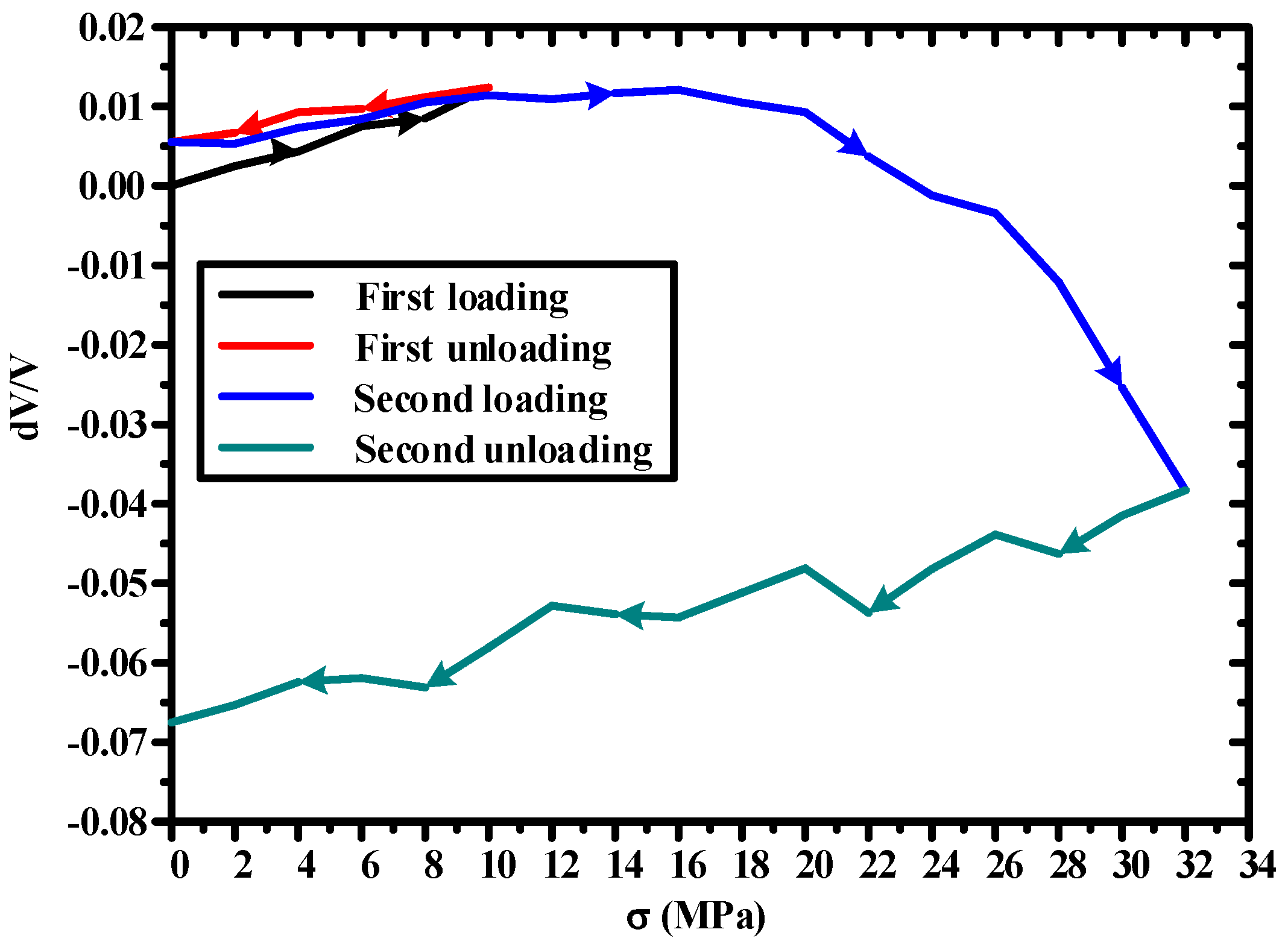
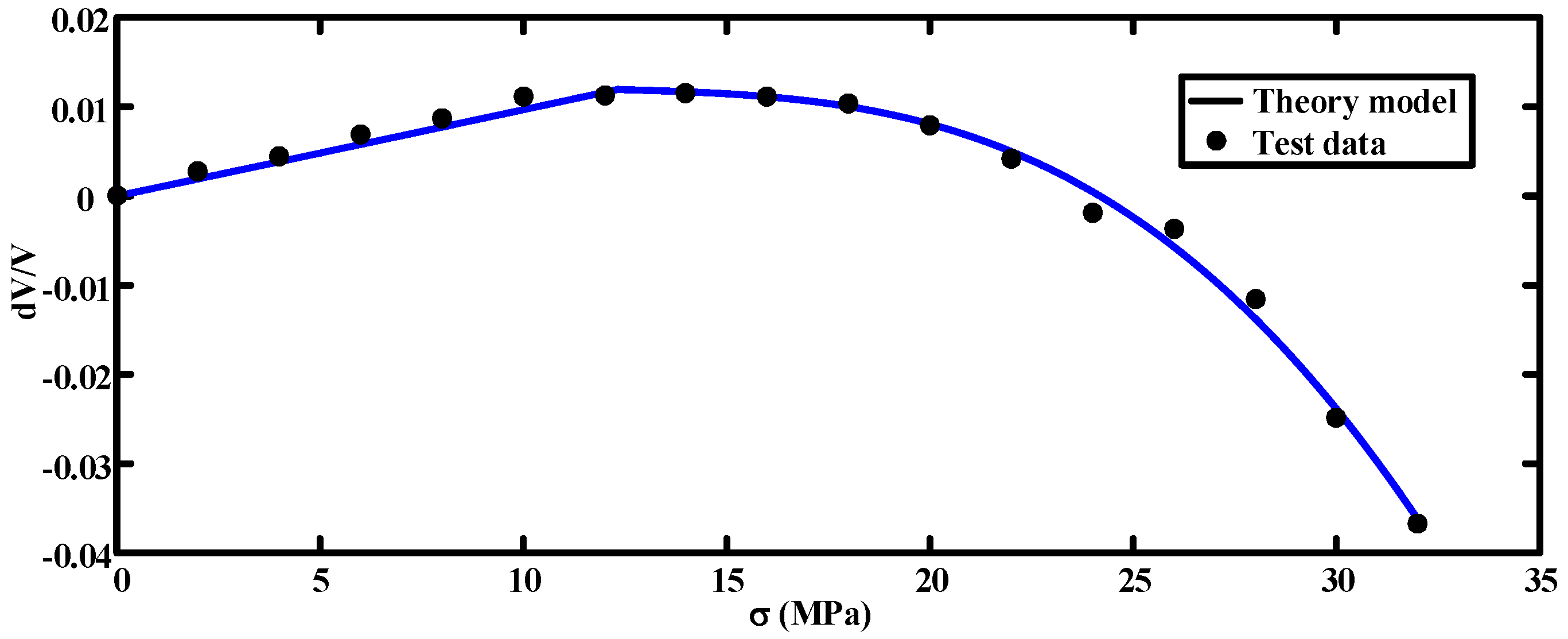
3.4.2. Relation between Stress and Coda Wave Velocity

Figure 9 illustrates the experimental curves of the relation between the relative variation of axial sound velocity and the stress on the specimen C-1-1. It was found that the axial sound velocity increases with the increase of stress in the process of loading from 0 MPa to 10 MPa. This is because the sound velocity in the pores is far less than that in the concrete matrix. Under the action of the stress, the microcracks in the concrete begin to close, resulting in the decrease of the porosity and the increase of the sound velocity. The sound velocity starts to decrease during the unloading process from 10 MPa to 0 MPa. After unloading completely, the sound velocity increases by approximately 2.15% compared to that at the initial time without loading. This is because the cracks are elastic, and in the process of unloading, the closed cracks start to recover and the sound velocity is reduced. When the specimen was unloaded to 0 MPa, a part of the closed cracks which did not have time to fully recover to the original state remained. Therefore, the corresponding wave velocity is larger than that at the initial time. Then, the specimen was loaded from 0 MPa until 32 MPa, approximately 75% of the concrete strength. In this process, after the maximum sound velocity increase by 7.35%, it begins to slow down, but the trend is not obvious, indicating that the cracks start to extend with the increase of stress, the porosity increases, and the wave velocity decreases. However, the secondary cracks generated by the crack growth form along the axial direction, and their influence on the horizontal sound velocity is large but the influence on the axial sound velocity is small, so the change of axial sound velocity is not obvious in the crack extended stage. Finally, the specimen was unloaded from 32 MPa to 0 MPa. In this process, the change of the axial sound velocity is not obvious, but still has a downward trend. This is because when the concrete is loaded at a high stress level, the cracks are in an unstable situation. After unloading, the cracks continue to extend. Therefore, the axial sound velocity has a downward trend. In the whole process, the maximum sensitivity is 1 MPa, and the change in the wave velocity (dV/V) is 0.00885.

In Figure 10, the relation between the horizontal sound velocity and the stress on the specimen C-2-1 is shown. It was found that the horizontal sound velocity increases with the increase of stress in the process of loading from 0 MPa to 10 MPa, but the change is not obvious. This is because when the microcracks are in the closed stage, their lateral deformation is much smaller than their axial deformation. The closed cracks begin to recover during the unloading process from 10 MPa to 0 MPa. After unloading to 0 MPa, the sound velocity is increased by about 0.55% compared to that at the initial time without loading. This is also because a part of the closed cracks remains, as they may not have time to fully recover to the original state. Then the specimen was observed with loading from 0 MPa to 32 MPa. After the sound velocity reaches the maximum value, it begins to decrease sharply. The maximum sound velocity is about 1.21% larger than that at the initial time. This is because the cracks begin to extend as the stress increases. The secondary cracks are along the axial direction, which has a great influence on the horizontal sound velocity, so the horizontal sound velocity in the crack extended stage decreases sharply. Finally, the specimen was unloaded from 32 MPa to 0 MPa. In this process, the cracks are in an unstable extended stage. After unloading, the cracks will continue to extend and the horizontal sound velocity will continue to decrease. After unloading to 0 MPa, the sound velocity is about 6.75% lower than that at the initial moment. In the whole process, the maximum sensitivity is 1 MPa, and the change in the wave velocity (dV/V) is 0.00095.

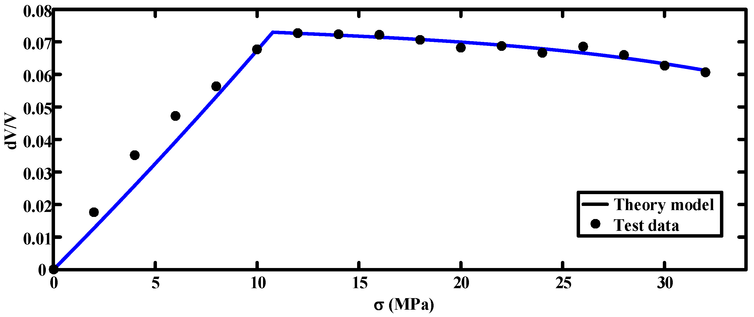
3.4.3. Data Processing and Parameter Fitting

According to the CWI analysis method, we calculated the wave velocity change of different stress levels. The least square method was used to fit the parameters $k_{\mathrm{c}1}$, $k_{\mathrm{f}1}$, $k_{\mathrm{f}2}$, $k_{\mathrm{c}2}$, $k_{\mathrm{f}21}$, and $k_{\mathrm{f}22}$ in Equation (22). The data from the increasing stage of the sound velocity change was used to fit $k_{\mathrm{c}1}$ and $k_{\mathrm{c}2}$ in Equations (22a) and (22c), and the data from point at which the change of sound velocity begins to decline was used to fit $k_{\mathrm{f}1}$, $k_{\mathrm{f}2}$, $k_{\mathrm{f}21}$, and $k_{\mathrm{f}22}$ in Equations (22b) and (22d). The fitting results are given in

Table 3. Fitting results of axial crack parameters.

Model Parameter	Fitted Value	Correlation Coefficient R
$k_{\mathrm{c}1}$	6.314 × 10−3	0.9359
$k_{\mathrm{f}11}$	2.395 × 10−4	0.9109
$k_{\mathrm{f}12}$	5.454 × 10−7
${\sigma }_{\mathrm{u}}$	10.77

and

Table 4. Fitting results of horizontal crack parameters.

Model Parameter	Fitted Value	Correlation Coefficient R
$k_{\mathrm{c}2}$	9.58 × 10−4	0.9237
$k_{\mathrm{f}21}$	1.326 × 10−4	0.9915
$k_{\mathrm{f}22}$	6.147 × 10−6
${\sigma }_{\mathrm{u}}$	12.33

.

After inserting the fitted parameters into the models, we obtain:

Axial relative sound velocity:

Crack closure stage

$$\frac{\Delta V_1}{V_{\mathrm{p}0}}=\frac{1}{1-6.314\times {10}^{-3}\sigma }-1$$

(25a)

Crack expansion stage

$$\frac{\Delta V_1}{V_{\mathrm{p}0}}=\frac{1}{0.9320+2.395\times {10}^{-4}\times (\sigma -10.77)+5.454\times {10}^{-7}\times {(\sigma -10.77)}^3}-1$$

(25b)

The horizontal sound velocity can be expressed as:

Crack closure stage

$$\frac{\Delta V_2}{V_{\mathrm{p}0}}=\frac{1}{1-9.58\times {10}^{-4}\sigma }-1$$

(25c)

Crack expansion stage

$$\frac{\Delta V_2}{V_{\mathrm{p}0}}=\frac{1}{0.9882-1.326\times {10}^{-4}(\sigma -12.33)+6.147\times {10}^{-6}{(\sigma -12.33)}^3}-1$$

(25d)

Compared with the experimental data, as shown in Figure 11 and Figure 12, it was found that the results obtained by the fitted model agree well with the experimental data, indicating that the proposed model can reflect the propagation law of ultrasonic wave when stress changes in concrete.

4. Discussion

From the perspective of microcrack deformation, this paper proposed a model to simulate the relation between the sound velocity and stress in concrete, and the relevant parameters in the model were fitted using the CWI analysis method. Finally, the specific expression of the relation between the sound velocity and uni-axial stress of concrete was obtained.

In practical engineering, to obtain the stress $\sigma$ or stress increment $\Delta \sigma$ in a concrete structure, the following steps are required:

Step 1.

Conduction of field test or laboratory experiment on unloaded concrete to obtain the initial waveform of the coda wave;

Step 2.

Calibration or regression of the parameters in Equation (22);

Step 3.

Conduction of field test on loaded concrete structures to obtain the waveform of the coda wave;

Step 4.

Analysis of the obtained coda wave by the wave expansion method to determine the relative change between the sound velocity $\Delta V/V_{p0}$;

Step 5.

Determine the stress $\sigma$ (or stress increment $\Delta \sigma$) using Equation (22) with calibrated parameters.

Conventional ultrasonic testing methods usually use the duration of direct wave propagation in concrete to calculate the wave velocity; however, this approach has a low accuracy due to two main reasons: (1) the measurement of the duration of direct waves in concrete is easily affected by the timing error of the instrument; and (2) it is difficult to overcome the obstacles caused by the multiple components and inhomogeneity of concrete, and the energy will attenuate rapidly. The coda wave formed by multiple scattering can overcome these defects, and the accuracy of the calculation is much higher than that of the traditional methods. CWI technology calculates the wave velocity through the processing of the whole waveform along the time axis, which can avoid the error of point measurements and achieve high-precision and more stable results. At the same time, in complex media, the coda wave is better developed than that in homogeneous materials. Therefore, it is more suitable for the detection of structural changes in concrete. In this paper, the sensitivity calculated by the CWI analysis method reached dV/V = 0.00095/MPa. However, it is notable that the measurement of CWI is the average effect of the stress on the path of sound wave propagation, while the spatial resolution is weak. Moreover, the temperature and humidity can also influence the wave velocity, resulting in error of stress estimation. The authors suggest that the results of CWI should be corrected by considering the temperature and humidity in the model in future research.

To establish a quantitative relation between the change of the coda wave and stress (or stress increment) in concrete structures, crack was selected to be the medium between the stress and coda wave. For the method used to describe the influence of stress on concrete cracks, both the closure and expansion of existing cracks were considered. The fundamental principle of the method was referred from Walsh’s study in 1965 [23], which is a classical method adopted by many researches. In the proposed model describing the crack propagation, concrete was treated as a linearly elastic material, like rocks. Pores in concrete were simplified as ellipses, and they would close or expand while loads were applied on the material. The influence of cracks and concrete material properties on the sound velocity would be independent with each other, which would lead to a much more simplified and logical derivation of the theoretical formula, as compared to some other concrete crack models, such as the fictitious crack model and adhesive crack model. However, there are many factors that could influence the shape of cracks, indicating that some parameters in the proposed model have to be regressed or calibrated by the test results.

5. Conclusions

In this paper, the feasibility of measuring stresses in concrete by the CWI technique was studied and discussed. The correlation model of sound velocity and stress in concrete was established on the basis of acoustoelastic theory. Moreover, the development law of the coda wave in concrete was illustrated by experiments. The model with regressed parameters can describe the corresponding relation between the velocity change of the coda wave and stress well. The findings can also indicate that the coda wave formed by multiple scattering has a higher accuracy in detecting changes in the properties of the concrete material than does the direct wave method.

References

1. Porco, F.; Fiore, A.; Porco, G.; Uva, G. Monitoring and safety for prestressed bridge girders by SOFO sensors. J. Civ. Struct. Heal. Monit. 2012, 3, 3–18. [Google Scholar] [CrossRef]
2. Zhang, F.P.; Qiu, Z.G. Analysis of measuring existing stresses in concrete structure by hole drilling core surface strain gauge method. Mater. Res. Innov. 2011, 15, s601–s604. [Google Scholar] [CrossRef]
3. Trautner, C.A.; Mcginnis, M.J.; Pessiki, S.P. The incremental core drilling method to determine in-situ stresses in concrete. ACI Mater. J. 2011, 8, 85–94. [Google Scholar]
4. McCann, D.M.; Forde, M.C. Review of NDT methods in the assessment of concrete and masonry structures. NDT E Int. 2001, 34, 71–84. [Google Scholar] [CrossRef]
5. Invernizzi, S.; Lacidogna, G.; Carpinteri, A. Numerical models for the assessment of historical masonry structures and materials, monitored by acoustic emission. Appl. Sci. 2016, 6, 102. [Google Scholar] [CrossRef]
6. Planès, T.; Larose, E. A review of ultrasonic Coda Wave Interferometry in concrete. Cem. Concr. Res. 2013, 53, 248–255. [Google Scholar] [CrossRef]
7. Hertlein, B.H. Stress wave testing of concrete: A 25-year review and a peek into the future. Constr. Build. Mater. 2013, 38, 1240–1245. [Google Scholar] [CrossRef]
8. Mutlib, N.K.; Baharom, S.B.; El-Shafie, A.; Nuawi, M.Z. Ultrasonic health monitoring in structural engineering: Buildings and bridges. Struct. Control Heal. Monit. 2016, 23, 409–422. [Google Scholar] [CrossRef]
9. Niederleithinger, E.; Taffe, A. Early stage elastic wave velocity of concrete piles. Cem. Concr. Compos. 2006, 28, 317–320. [Google Scholar] [CrossRef]
10. Aggelis, D.G.; Shiotani, T.; Philippidis, T.P.; Polyzos, D. Stress wave scattering: An enemy or friend of non-destructive testing of Concrete? J. Solid Mech. Mater. Eng. 2008, 2, 397–408. [Google Scholar] [CrossRef]
11. Snieder, R. The theory of coda wave interferometry. Pure Appl. Geophys. 2006, 163, 455–473. [Google Scholar] [CrossRef]
12. Aki, K. Analysis of the seismic coda of local earthquakes as scattered waves. J. Geophys. Res. 1969, 74, 615–631. [Google Scholar] [CrossRef]
13. Snieder, R.; Grêt, A.; Douma, H.; Scales, J. Coda wave interferometry for estimating nonlinear behavior in seismic velocity. Science 2002, 295, 2253–2255. [Google Scholar] [CrossRef] [PubMed]
14. Lobkis, O.I.; Weaver, R.L. Coda-wave interferometry in finite solids: Recovery of P-to-S conversion rates in an elastodynamic billiard. Phys. Rev. Lett. 2003, 90, 254302. [Google Scholar] [CrossRef] [PubMed]
15. Larose, E.; Hall, S. Monitoring stress related velocity variation in concrete with a 2 × 10⁻⁵ relative resolution using diffuse ultrasound. J. Acoust. Soc. Am. 2009, 125, 1853–1856. [Google Scholar] [CrossRef] [PubMed]
16. Larose, E.; de Rosny, J.; Margerin, L.; Anache, D.; Gouedard, P.; Campillo, M.; van Tiggelen, B. Observation of multiple scattering of kHz vibrations in a concrete structure and application to monitoring weak changes. Phys. Rev. E 2006, 73, 016609. [Google Scholar] [CrossRef] [PubMed]
17. Schurr, D.P.; Kim, J.Y.; Sabra, K.G.; Jacobs, L.J. Damage detection in concrete using coda wave interferometry. NDT E Int. 2011, 44, 728–735. [Google Scholar] [CrossRef]
18. Lillamand, I.; Chaix, J.F.; Ploix, M.A.; Garnier, V. Acoustoelastic effect in concrete material under uni-axial compressive loading. NDT E Int. 2010, 43, 655–660. [Google Scholar] [CrossRef]
19. Niederleithinger, E.; Sens-Schönfelder, C.; Grothe, S.; Wiggenhauser, H. Coda Wave Interferometry used to localize compressional load effects in a concrete specimen. In Proceedings of the EWSHM-7th European Workshop on Structural Health Monitoring, Nates, France, 1 July 2014. [Google Scholar]
20. Stähler, S.C.; Sensschönfelder, C.; Niederleithinger, E. Monitoring stress changes in a concrete bridge with coda wave interferometry. J. Acoust. Soc. Am. 2011, 129, 1945–1952. [Google Scholar] [CrossRef] [PubMed]
21. Chronopoulos, D. Wave steering effects in anisotropic composite structures: Direct calculation of the energy skew angle through a finite element scheme. Ultrasonics 2017, 73, 43–48. [Google Scholar] [CrossRef] [PubMed] [Green Version]
22. Zhang, Y.; Fu, L.Y.; Zhang, L.; Wei, W.; Guan, X. Finite difference modeling of ultrasonic propagation (coda waves) in digital porous cores with un-split convolutional PML and rotated staggered grid. J. Appl. Geophys. 2014, 104, 75–89. [Google Scholar] [CrossRef]
23. Walsh, J.B. The effect of cracks on the compressibility of rock. J. Geophys. Res. 1965, 70, 381–389. [Google Scholar] [CrossRef]
24. Minato, S.; Tsuji, T.; Ohmi, S.; Matsuoka, T. Monitoring seismic velocity change caused by the 2011 Tohoku-oki earthquake using ambient noise records. Geophys. Res. Lett. 2012, 39, L09309–L09314. [Google Scholar] [CrossRef]
Figure 1. Sound velocity equivalent model of concrete with microcracks under the zero stress state.
Applsci 08 01609 g001
Figure 2. Close of a compression-shear crack.
Applsci 08 01609 g002
Figure 3. Concrete contains a set of horizontal microcracks.
Applsci 08 01609 g003
Figure 4. Equipment used for the experiment.
Applsci 08 01609 g004
Figure 5. Reception waveform of acoustic signals with different frequencies: (a) 300 kHz, (b) 150 kHz, (c) 50 kHz.
Applsci 08 01609 g005
Figure 6. Frequency spectrum of the received signal at different frequencies: (a) 300 kHz, (b) 150 kHz.
Applsci 08 01609 g006
Figure 7. Received waveform of sensors at different locations: (a) opposite side, (b) top.
Applsci 08 01609 g007aApplsci 08 01609 g007b
Figure 8. Comparison of the received waveforms between 0 MPa and 2 MPa. (a,b) Time window A, (c) time window B, (d) time window C.
Applsci 08 01609 g008
Figure 9. Relation between the relative change of axial velocity and stress.
Applsci 08 01609 g009
Figure 10. Relation between the relative change of horizontal sound velocity and stress.
Applsci 08 01609 g010
Figure 11. Comparison between the proposed model and experimental data of the axial sound velocity ratio.
Applsci 08 01609 g011
Figure 12. Comparison between the proposed model and experimental data of the horizontal sound velocity ratio.
Applsci 08 01609 g012