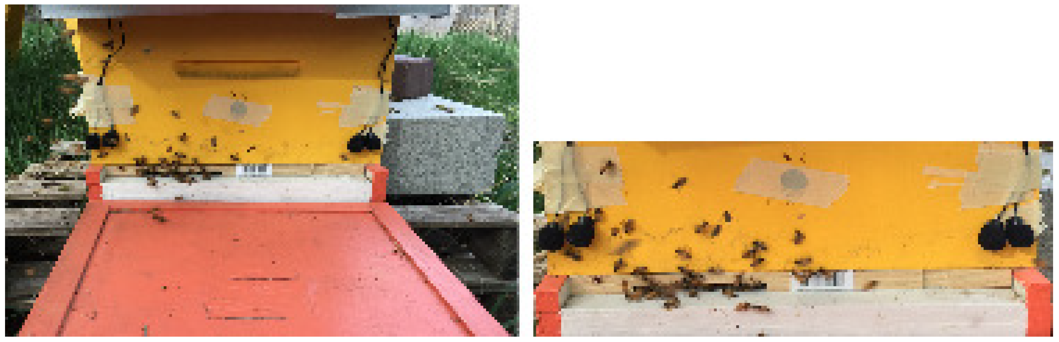
Article

Toward Audio Beehive Monitoring: Deep Learning vs. Standard Machine Learning in Classifying Beehive Audio Samples

Department of Computer Science, Utah State University, 4205 Old Main Hill, Logan, UT 84322-4205, USA
*
Author to whom correspondence should be addressed.
Appl. Sci. 2018, 8(9), 1573; https://doi.org/10.3390/app8091573
Submission received: 31 May 2018 / Revised: 29 August 2018 / Accepted: 30 August 2018 / Published: 6 September 2018

Abstract

:

Abstract

Electronic beehive monitoring extracts critical information on colony behavior and phenology without invasive beehive inspections and transportation costs. As an integral component of electronic beehive monitoring, audio beehive monitoring has the potential to automate the identification of various stressors for honeybee colonies from beehive audio samples. In this investigation, we designed several convolutional neural networks and compared their performance with four standard machine learning methods (logistic regression, k-nearest neighbors, support vector machines, and random forests) in classifying audio samples from microphones deployed above landing pads of Langstroth beehives. On a dataset of 10,260 audio samples where the training and testing samples were separated from the validation samples by beehive and location, a shallower raw audio convolutional neural network with a custom layer outperformed three deeper raw audio convolutional neural networks without custom layers and performed on par with the four machine learning methods trained to classify feature vectors extracted from raw audio samples. On a more challenging dataset of 12,914 audio samples where the training and testing samples were separated from the validation samples by beehive, location, time, and bee race, all raw audio convolutional neural networks performed better than the four machine learning methods and a convolutional neural network trained to classify spectrogram images of audio samples. A trained raw audio convolutional neural network was successfully tested in situ on a low voltage Raspberry Pi computer, which indicates that convolutional neural networks can be added to a repertoire of in situ audio classification algorithms for electronic beehive monitoring. The main trade-off between deep learning and standard machine learning is between feature engineering and training time: while the convolutional neural networks required no feature engineering and generalized better on the second, more challenging dataset, they took considerably more time to train than the machine learning methods. To ensure the replicability of our findings and to provide performance benchmarks for interested research and citizen science communities, we have made public our source code and our curated datasets.

Dataset

The curated datasets for this article (BUZZ1 and BUZZ2) are publicly available at https://usu.app.box.com/v/BeePiAudioData; Python source code for data capture is publicly available at https://github.com/VKEDCO/PYPL/tree/master/beepi/py/src/29Jan2016; Python source code for the deep learning and machine learning experiments is publicly available at https://github.com/sarba-jit/EBM_Audio_Classification.

1. Introduction

Many beekeepers listen to their hives to ascertain the state of their honey bee colonies because bee buzzing carries information on colony behavior and phenology. Honey bees generate specific sounds when exposed to stressors such as failing queens, predatory mites, and airborne toxicants [1]. While experienced beekeepers can tell audio changes in sounds produced by stressed colonies, they may not always be able to determine the exact causes of the changes without hive inspections. Unfortunately, hive inspections disrupt the life cycle of bee colonies and put additional stress on the bees. The transportation costs are also a factor because many beekeepers drive long distances to their far flung apiaries due to increasing urban and suburban sprawls. Since beekeepers cannot monitor their hives continuously due to obvious problems with logistics and fatigue, a consensus is emerging among researchers and practitioners that electronic beehive monitoring (EBM) can help extract critical information on colony behavior and phenology without invasive beehive inspections and transportation costs [2]. When viewed as a branch of ecoacoustics [3], an emerging interdisciplinary science that investigates natural and anthropogenic sounds and their relations with the environment, audio beehive monitoring contributes to our understanding of how beehive sounds reflect the states of beehives and the environment around them.
In this article, we contribute to the body of research on audio beehive monitoring by comparing several deep learning (DL) and standard machine learning (ML) methods in classifying audio samples from microphones deployed approximately 10 cm above Langstroth beehives’ landing pads. In our experiments, the convolutional neural networks (ConvNets) performed on par with or better than the four standard ML methods on two curated datasets. On the first dataset of 10,260 audio samples (BUZZ1) where the training and testing samples were separated from the validation samples by beehive and location, a shallower raw audio ConvNet with a custom layer outperformed three deeper raw audio ConvNets without custom layers and performed on par with the four ML methods trained to classify feature vectors extracted from raw audio samples. On the second, more challenging dataset of 12,914 audio samples (BUZZ2) where the training and testing samples were separated from the validation samples by beehive, location, time, and bee race, all raw audio convolutional neural networks performed better than the four ML methods and a ConvNet trained to classify spectrogram images of raw audio samples obtained through Fourier analysis [4,5].
Our investigation gives an affirmative answer to the question of whether ConvNets can be used in real electronic beehive monitors that use low voltage devices such as Raspberry Pi [6] or Arduino [7]. Toward this end, we demonstrate that trained ConvNets can operate in situ on a credit card size Raspberry Pi computer. The presented methods do not depend on the exact positioning of microphones, and can be applied to any audio samples obtained from microphones placed inside or outside beehives provided that microphone propolization is controlled for. Our objective is to develop open source software tools for researchers, practitioners, and citizen scientists who want to capture and classify their audio beehive samples. To ensure the replicability of our findings and to establish performance benchmarks for interested research and citizen science communities, we have made public our two curated datasets, BUZZ1 (10,260 samples) and BUZZ2 (12,914 samples), of manually labeled audio samples (bee buzzing, cricket chirping, and ambient noise) used in this investigation [8].

2. Background

As an integral component of EBM, audio beehive monitoring has attracted considerable research and development effort. Bromenschenk et al. [1] designed a system for profiling acoustic signatures of honeybee colonies, analyzing these signatures, and identifying various stressors for the colonies from this analysis. A foam insulated microphone probe assembly is inserted through a hole drilled in the back of the upper super of a Langstroth hive that consists of two supers. The hole is drilled so that the probe is inserted between honeycomb frames at least four inches down from the top of the upper super, because brood frames are typically located in the two lower supers of a standard Langstroth hive. The probe’s microphone is connected via a microphone amplifier to a computer with an audio card and the audio analyzing software that performs the Fast Fourier Transform (FFT) of captured wav files and then saves the processed data to text files for subsequent analysis. The frequency spectrum is processed into a running average and an overall average. The two averages are exported to text-based files and are analyzed with statistical software to associate sound spectra with acoustic variations. In an experiment, bee colonies treated with naptha, ammonia, or toluene all produced statistically different scores with each stressor producing a unique acoustic signature. The researchers state that these associations can be detected with artificial neural networks (ANNs) but offer no experimental evidence of this claim.
Ferrari et al. [9] designed a system for monitoring swarm sounds in beehives. The system consisted of a microphone, a temperature sensor, and a humidity sensor placed in a beehive and connected to a computer in a nearby barn via underground cables. The sounds were recorded at a sample rate of 2 kHz and analyzed with Matlab. The researchers monitored three beehives for 270 h and observed that swarming was indicated by an increase of the buzzing frequency at about 110 Hz with a peak at 300 Hz when the swarm left the hive. Another finding was that a swarming period correlated with a rise in temperature from 33 °C to 35 °C with a temperature drop to 32 °C at the actual time of swarming.
Ramsey et al. [10] presented a method to analyze and identify honey bee swarming events through a computational analysis of acoustic vibrations captured with accelerometers placed on the outside walls of hives. The researchers placed two accelerometers on the outer walls of two Langstroth hives with Apis mellifera honey bees, one accelerometer per hive. A cavity was drilled in the center of the back wall of each hive. Both hives were located in close proximity to each other and approximately 10 m away from a house with a PC running a Linux distribution. The accelerometers were placed in the cavities and connected to a dual channel conditioner placed between the hives and encased in a waterproof acrylic box. The conditioner was coupled to the indoor PC with two coaxial cables through which the captured vibration samples were saved on the PC’s hard disk. An ad hoc roof was placed above both hives to control for vibrations caused by rain drops. The vibration samples, each one hour long, were logged from April to June 2009. Averaged frequency spectra were computed for a frequency resolution of 20 Hz and an averaging time of 510 s. The averaged spectra were combined into one day long spectrograms which were analyzed with the Principal Component Analysis (PCA) for feature extraction. The witnessed swarming events were juxtaposed with the corresponding spectrograms and were found to exhibit a unique set of features. A subsequent minimization computer analysis suggested that swarming may be detected several days in advance. Peaks in vibrational activities were discovered at 250 Hz, 500 Hz, 750 Hz, and 2000 Hz.
Mezquida and Martinez [11] developed a distributed audio monitoring system for apiaries. The system consists of nodes and wireless sensor units with one node per apiary and one sensor unit per hive. A node is a solar-powered embedded computer. A sensor unit consists of an omnidirectional microphone and a temperature sensor. Sensor units are placed at the bottom of each hive protected by a grid to prevent propolization. The system was tested in an apiary of 15 Langstroth hives where up to 10 hives were monitored continuously by taking 8 s audio samples every hour with a sampling rate of 6250 Hz. The timestamped frequency spectra obtained with Fourier transform and temperature data were logged in a SQL database from May 2008 to April 2009. The researchers reported that sound volume and sound intensity at medium and low frequencies showed distinguishable daily patterns, especially in the spring. Sound volume did not have identifiable patterns in the winter.
Rangel and Seeley [12] also investigated audio signals of honeybee swarms. Five custom designed observation hives were sealed with glass covers. The captured video and audio data were monitored daily by human observers. By manually analyzing the captured audio samples and correlating them with the corresponding video samples, the researchers found that approximately one hour before swarm exodus, the production of piping signals gradually increased and ultimately peaked at the start of the swarm departure.
Kulyukin et al. [13] designed an algorithm for digitizing bee buzzing signals with harmonic intervals into A440 piano note sequences to obtain symbolic representations of buzzing signals over specific time periods. When viewed as a time series, such sequences correlate with other timestamped data such as estimates of bee traffic levels or temperatures [14,15]. The note range detected by the proposed algorithm on 3421.52 MB of 30-s wav files contained the first four octaves, with the lowest note being A0 and the highest note being F#4. It was observed that the peaks in the frequency counts, as the selected 24-h time period progressed, started in the first octave (D1), shifted higher to C3 and C#3 in the third octave, and returned back to the first octave at the end of the selected time period. Several notes in the fourth octave, e.g., F#4 and C#4, were also detected, but their frequency counts were substantially lower than those of the peaks in the first three octaves.
Representation learning is a branch of AI that investigates automatic acquisition of representations from raw signals for detection and classification [16]. Standard machine learning (ML) techniques are believed to be limited in their ability to acquire representations from raw data because they require considerable feature engineering to convert raw signals into feature vectors used in classification. Unlike conventional ML techniques, deep learning (DL) methods are believed to be better at acquiring multi-layer representations from raw data because real data often encode non-linear manifolds that low-order functions have a hard time modeling. In a DL architecture, each layer, starting from raw input, can be construed as a function transforming its input to the one acceptable for the next layer. Many features of these layers are learned automatically by a general purpose procedure known as backpropagation [17]. DL methods have been successfully applied to image classification [18,19,20], speech recognition and audio processing [21,22], music classification and analysis [23,24,25], environmental sound classification [26], and bioinformatics [27,28].
Convolutional neural networks (ConvNets) are a type of DL feedforward neural networks that have been shown in practice to better train and generalize than artificial neural networks (ANNs) on large quantities of digital data [29]. In ConvNets, filters of various sizes are convolved with a raw input signal to obtain a stack of filtered signals. This transformation is called a convolution layer. The size of a convolution layer is equal to the number of convolution filters. The convolved signals are typically normalized. A standard choice for signal normalization is the rectified linear unit (ReLU) that converts all negative values to 0’s [30,31,32]. A layer of normalization units is called a normalization layer. Some ConvNet architectures (e.g., [26]) consider normalization to be part of convolution layers. The size of the output signal from a layer can be downsampled with a maxpooling layer, where a window is shifted in steps, called strides, across the input signal retaining the maximum value from each window. The fourth type of layer in a ConvNet is a fully connected (FC) layer, where the stack of processed signals is treated as a 1D vector so that each value in the output from a previous layer is connected via a synapse (a weighted connection that transmits a value from one unit to another) to each node in the next layer. In addition to the four standard layers, ConvNets can have custom layers that implement arbitrary functions to transform signals between consecutive layers.
Since standard and custom layers can be stacked arbitrarily deeply and in various permutations, ConvNets can model highly non-linear manifolds. The architectural features of a ConvNet that cannot be dynamically changed through backpropagation are called hyperparameters and include the number and size of filters in convolution layers, the window size and stride in maxpooling layers, and the number of neurons in FC layers. These permutations and hyperparameters distinguish one ConvNet architecture from another.
In audio processing, ConvNets have been trained to classify audio samples either by classifying raw audio or vectors of various features extracted from raw audio. For example, Piczak [26] evaluated the potential of ConvNets to classify short audio samples of environmental sounds by developing a ConvNet that consisted of two convolution layers with maxpooling and two FC layers. The ConvNet was trained on the segmented spectrograms of audio data. When evaluated on three public datasets of environmental and urban recordings, the ConvNet outperformed a baseline obtained from random forests with mel frequency cepstral coefficients (MFCCs) and zero crossing rates and performed on par with some state-of-the-art audio classification approaches. Aytar et al. [33] developed a deep ConvNet to learn directly from raw audio waveforms. The ConvNet was trained by transferring knowledge from computer vision to classify events from unlabeled videos. The representation learned by the ConvNet obtained state-of-the-art accuracy on three standard acoustic datasets. In [34], van den Oord et al. showed that generative networks can be trained to predict the next sample in an audio sequence. The proposed network consisted of 60 layers and sampled raw audio at a rate of 16 kHz to 48 kHz. Humphrey and Bello [35] designed a ConvNet to classify 5-s tiles of pitch spectra to produce an optimized chord recognition system. The ConvNet yielded state-of-the-art performance across a variety of benchmarks.

3. Materials and methods

3.1. Hardware

All audio data for this investigation were captured by BeePi, a multi-sensor EBM system we designed and built in 2014 [13]. A fundamental objective of the BeePi design is reproducibility: other researchers and citizen scientists should be able to replicate our results at minimum costs and time commitments. Each BeePi monitor consists of exclusively off-the-shelf components: a Raspberry Pi computer, a miniature camera, a microphone splitter, four microphones connected to a splitter, a solar panel, a temperature sensor, a battery and a hardware clock. We currently use Raspberry Pi 3 model B v1.2 computers, Pi T-Cobblers, breadboards, waterproof DS18B20 digital temperature sensors, and Pi cameras. Each BeePi unit is equipped with four Neewer 3.5 mm mini lapel microphones that are placed either above the landing pad or embedded in beehive walls. These microphones have a frequency range of 15–20 KHz, an omnidirectional polarity, and a signal-to-noise ratio greater than 63 dB. There are two versions of BeePi: solar and regular. In the solar version, a solar panel is placed either on top of or next to a beehive. For solar harvesting, we use Renogy 50 watts 12 Volts monocrystalline solar panels, Renogy 10 Amp PWM solar charge controllers, and Renogy 10 ft 10 AWG solar adaptor kits. The regular version operates either on the grid or on a rechargeable battery. For power storage, we use two types of rechargeable batteries: the UPG 12 V 12 Ah F2 lead acid AGM deep cycle battery and the Anker Astro E7 26,800 mAh battery. All hardware components, except for solar panels, are placed in a Langstroth super. Interested readers are referred to [36] for BeePi hardware design descriptions, pictures, and assembly videos.
We have been iteratively improving the BeePi hardware and software since 2014. BeePi monitors have so far had five field deployments. The first deployment was in Logan, UT, USA (September 2014) when a BeePi monitor was placed into an empty hive and ran exclusively on solar power for two weeks. The second deployment was in Garland, UT, USA (December 2014–January 2015) when a BeePi monitor was placed in a hive with overwintering honey bees and successfully operated for nine out of the fourteen days of deployment exclusively on solar power and captured about 200 MB of data. The third deployment was in North Logan, UT, USA (April 2016–November 2016) where four BeePi monitors were placed into four beehives at two small apiaries and collected 20 GB of data. The fourth deployment was in both Logan and North Logan, UT, USA (April 2017–September 2017) when four BeePi units again placed into four beehives at two small apiaries to collect 220 GB of audio, video, and temperature data [15]. The fifth deployment started in Logan, UT, USA in May 2018 with four BeePi monitors placed in four new beehives freshly initiated with Carniolan honeybee colonies. As of July 2018, we collected 66.04 GB of data.

3.2. Audio Data

The audio data for this investigation were taken from the datasets captured by six BeePi monitors. Two BeePi monitors were deployed in Logan, UT, USA (41.7370° N, 111.8338° W) and the other two in North Logan, UT, USA (41.7694° N, 111.8047° W) from April 2017 to September 2017 in four Langstroth beehives with Italian honey bee colonies. The fifth and sixth BeePi monitors were deployed in Langstroth beehives with two freshly installed Carniolan colonies in Logan, UT, USA (41.7370° N, 111.8338° W) from May 2018 to July 2018. In a previous investigation [13], we reported on some advantages and disadvantages of embedding microphones into hive walls and insulating them against propolization with small metallic mesh nets. In this study, the microphones were placed approximately 10 cm above the landing pad with two microphones on each side (see Figure 1).
Each monitor saved a 30-s audio wav file every 15 min recorded with the four microphones above the beehives’ landing pads and connected to a Raspberry Pi computer. We experimentally found these two parameters (30 s every 15 min) to be a reasonable compromise between the continuity of monitoring and the storage capacity of a BeePi monitor. In a BeePi monitor, all captured data are saved locally either on the Raspberry Pi’s sdcard or on a USB storage device connected to the Raspberry Pi. No cloud computing facilities are used for data storage or analysis. Each 30-s audio sample was segmented into 2-s wav samples with a 1-s overlap, resulting in 28 2-s wav samples per one 30-s audio file. Data collection software is written in Python 2.7 [37].
We obtained the ground truth classification by manually labeling 9110 2-s audio samples captured with four BeePi monitors in two apiaries (one in Logan, UT, USA and one in North Logan, UT, USA ) in May and June 2017. The two apiaries were approximately seventeen kilometers apart. The first apiary (apiary 1) was in a more urban environment in Logan, UT, USA . In this apiary, the first monitored beehive (beehive 1.1) was placed next to a garage with a power generator. The second monitored beehive (beehive 1.2) was placed approximately twenty meters west of beehive 1.1 behind a row of aspens and firs where the generator’s sound was less pronounced. However, beehive 1.2 was located closer to a large parking lot. Hence, some audio samples from beehive 1.2 contained sounds of car engines and horns. Some samples from beehives 1.1 and 1.2 contained sounds of fire engine or ambulance sirens. In May 2018, two more Langstroth beehives (beehive 1.3 and beehive 1.4) were added to apiary 1 to obtain the validation data for BUZZ2 (see below for details). The second apiary (apiary 2) was in a more rural area in North Logan, UT, USA, seventeen kilometers north of apiary 1. In this apiary, we collected the data from two monitored beehives located approximately fifteen meters apart. Each beehive was located next to an unmonitored beehive. The first monitored beehive in apiary 2 (beehive 2.1) was placed close to a big lawn. The lawn was regularly mowed by the property owner and watered with an automated sprinkler system. The second monitored beehive in apiary 2 (beehive 2.2) was located fifteen meters west of beehive 2.1, deeper in the backyard where ambient noise (sprinklers, mower’s engine, children playing on the lawn, human conversation) was barely audible. The validation dataset of BUZZ2 used for model selection was obtained from two Langstroth beehives (1.3 and 1.4) in apiary 1 obtained in May 2018.
We listened to each sample and placed it into one of the three non-overlapping categories: bee buzzing (B), cricket chirping (C), and ambient noise (N). The B category consisted of the samples where at least two of us could hear bee buzzing. The C category consisted of the audio files captured at night where at least two of us could hear the chirping of crickets and no bee buzzing. The N category included all samples where none of us could clearly hear either bee buzzing or cricket chirping. These were the samples with sounds of static microphone noise, thunder, wind, rain, vehicles, human conversation, sprinklers, and relative silence, i.e., absence of any sounds discernible to a human ear. We chose these categories for the following reasons. The B category is critical in profiling acoustic signatures of honeybee colonies to identify various colony stressors. The C category is fundamental in using audio classification as a logical clock because cricket chirping is cyclical, and, in Northern Utah, is present only from 11:00 p.m. until 6:00 a.m. The N category helps EBM systems to identify uniquely individual beehives because ambient noise varies greatly from location to location and from beehive to beehive at the same location.
The first labeled dataset, which we designated to be our train/test dataset, included 9110 samples from beehives 1.1 and 2.1: 3000 B samples, 3000 C samples, and 3110 N samples. We later labeled another dataset, which we designated to be our validation dataset, of 1150 audio samples (300 B samples, 350 N samples, and 500 C samples) captured from beehives 1.2 and 2.2 in May and June 2017. Thus, the audio samples in the validation dataset were separated from the audio samples in the training and testing dataset by beehive and location. In summary, our first curated dataset, which we called BUZZ1 [8], consisted of 10,260 audio samples: a train/test dataset of 9110 samples that we used in our train/test experiments and a validation dataset of 1150 audio samples that we used in our validation experiments for model selection.
In BUZZ1, the degree of data overlap between the training and testing datasets in terms of the exact beehives being used is controlled for by the fact that audio samples from different beehives differ from each other even when the hives are located in the same apiary. To better control for data overlap, we created another curated dataset, BUZZ2 [8], of 12,914 audio samples where we completely isolated the training data from the testing data in terms of beehive and location by taking 7582 labeled samples (76.4%) for training from beehive 1.1 in apiary 1 and 2332 labeled samples (23.52%) samples for testing from beehive 2.1 in apiary 2. The training set of 7582 samples consisted of 2402 B samples, 3000 C samples, and 2180 N samples. The testing set of 2332 samples consisted of 898 B samples, 500 C samples, and 934 N samples. The validation dataset of BUZZ2 used for model selection was obtained from two Langstroth beehives (1.3 and 1.4) in apiary 1 obtained in May 2018. These beehives did not exist in apiary 1 in 2017. Both were freshly initiated with Carniolan honeybee colonies and started being monitored in May 2018. Thus, in BUZZ2, the train/test beehives were separated by beehive and location while the validation beehives were separated from the train/test beehives by beehive, location, time (2017 vs. 2018), and bee race (Italian vs. Carniolan). The validation dataset included 1000 B samples, 1000 C samples, and 1000 N samples.

3.3. Deep Learning

To obtain a baseline for our ConvNets that classify raw audio, we first developed a ConvNet architecture, called SpectConvNet, to classify spectrogram images of raw audio samples. In audio processing, a spectrogram represents an audio spectrum where time is represented along the x-axis and frequency along the y-axis and the strength of a frequency at each time frame is represented by color or brightness. Such spectrogram representations can be treated as RGB images. For example, Figure 2, Figure 3 and Figure 4 show spectrogram images of bee buzzing, cricket chirping, and ambient noise, respectively, computed from three audio samples from BUZZ1. The spectrograms were computed by using the specgram function from the Python matplotlib.pyplot package. This function splits an audio sample into NFFT = 512 length segments and the spectrum of each segment is computed. The number of overlap points between each segment was set to 384. The window size was 2048 and the hop size was 2048/4 = 512. The scaling frequency was the same as the input audio sample’s frequency. The windowed version of each segment was obtained with the default Hanning window function. Each spectrogram was converted to an 100 × 100 image with a dpi of 300. Thus, the time and frequency domains were treated equally, and were mapped to the range of [0, 99] each with each pixel value approximating a frequency value at a particular point in time.
The components of SpectConvNet are shown in Figure 5. Figure 6 shows a layer by layer control flow in SpectConvNet. Table 1 gives a detailed description of each layer of SpectConvNet. We trained SpectConvNet to classify 100 × 100 RGB spectrogram images such as the ones shown in Figure 2, Figure 3 and Figure 4. We chose the size of 100 × 100 experimentally as a compromise between accuracy and performance. The use of square filters in SpectConvNet’s layers was motivated by standard best practices in ConvNets trained to classify images (e.g., [18,20]). SpectConvNet has three convolution layers with ReLUs. In layer 1, the input is convolved using 100 3 × 3 filters (shown in red in Figure 6) with a stride of 1. The resultant 100 × 100 × 100 feature map is shown in layer 2 in red. The features are maxpooled with a kernel size of 2 resulting in a 50 × 50 × 100 feature map. The resultant feature map is processed with 200 3 × 3 filters (shown in blue in layer 2) with a stride of 1. The output is a 50 × 50 × 200 feature map (shown in blue in layer 3). In layer 3, another convolution is performed using 200 3 × 3 filters (shown in green) with a stride of 1. The result is a 50 × 50 × 200 feature map (shown in green in layer 4). The features are maxpooled with a kernel size of 2 resulting in a 25 × 25 × 200 feature map in layer 4. In layer 5, the output is passed through a 50-unit FC layer. In layer 6, a dropout [38] is applied with a keep probability of 0.5 to avoid overfitting and reduce complex co-adaptations of neurons [18]. Finally, the signal is passed through a 3-way softmax function that classifies it as bee buzzing (B), cricket chirping (C), or ambient noise (N).
After designing SpectConvNet, we followed some design suggestions from [26,35] to design a second ConvNet architecture, henceforth referred to as RawConvNet, to classify raw audio waveforms (see Figure 7). The layer by layer control flow on RawConvNet is shown in Figure 8. Table 2 gives a detailed description of each layer and its parameters.
RawConvNet consists of two convolution layers, both of which have 256 filters with ReLUs. The weights are randomly initialized using the methodology described by Xavier et al. in [39] to keep the scale of the gradients roughly the same in both layers. Each convolution layer has L2 regularization and a weight decay of 0.0001. The first convolution layer has a stride of 4, whereas the second layer has a stride of 1. A larger stride is chosen in layer 1 to lower the computation costs.
The input signal to RawConvNet is a raw audio wav file downsampled to 12 kHz and normalized to have a mean of 0 and a variance of 1. The raw audio file is passed as a 20,000 × 1 tensor to layer 1 (see Figure 8). In layer 1, the 1D tensor is convolved with 256 n × 1 filters (shown in red in layer 1) with a stride of 4 horizontally, where n ∈ {3, 10, 30, 80, 100}, and activated with ReLUs. We introduced the n parameter so that we could experiment with various receptive field sizes to discover their impact on classification, which we discuss in detail in Section 4 below. The resultant 5000 × 256 feature map is shown in layer 2 in red. Batch normalization [40] is applied to the resultant signal to reduce the internal covariate shift and the signal is maxpooled with a kernel size of 4 resulting in a 1250 ×256 feature map. The signal is convolved using 3 × 1 256 filters (shown in blue in layer 2) with a stride of 1 horizontally. The output is a 1250 × 256 feature map (shown in blue in layer 3). Batch normalization is applied again to the resultant signal and the signal is maxpooled with a kernel size of 4, resulting in a 313 × 256 feature map. In layer 4, we add a custom layer that calculates the mean of the resultant tensor of feature maps along the first axis. To put it differently, the custom layer is designed to calculate the global average over each feature map, thus reducing each feature map tensor to a single real number. The custom layer results in a 256 × 1 tensor (shown in magenta in layer 4). Finally, in layer 5, the output is passed through a 3-way softmax function that classifies it as B (bee buzzing), C (cricket chirping), or N (noise).

3.4. Standard Machine Learning

We used the following standard ML methods as comparison benchmarks for ConvNets: (M1) logistic regression [41]; (M2) k-nearest neighbors (KNN) [42]; (M3) support vector machine with a linear kernel one vs. rest (SVM OVR) classification [43]; and (M4) random forests [44]. These methods are supervised classification models that are trained on labeled data to classify new observations into one of the predefined classes.
The M1 model (logistic regression) is used for predicting dependent categorical variables that belong to one of a limited number of categories and assigns a class with the highest probability for each input sample. The M2 model (KNN) is a supervised learning model that makes no a priori assumptions about the probability distribution of feature vector values. The training samples are converted into feature vectors in the feature vector space with their class labels. Given an input sample, M2 computes the distances between the feature vector of an input sample and each feature vector in the feature vector space, and the input sample is classified by a majority vote of the classes of its k nearest neighbors, where k is a parameter. The M3 model (SVM OVR) builds a linear binary classifier for each class where n-dimensional feature vectors are separated by a hyperplane boundary into positive and negative samples, where negative samples are samples from other classes. Given an input sample, each classifier produces a positive probability of the input sample’s feature vector belonging to its class. The input sample is classified with the class of the classifier that produces the maximum positive probability. The M4 model (random forests) is an ensemble of decision trees where each decision tree is used to classify an input sample, and a majority vote is taken to predict the best class of the input sample.
We trained all four models on the same feature vectors automatically extracted from the raw audio files in BUZZ1. We used the following features: (F1) mel frequency cepstral coefficients (MFCC) [45]; (F2) chroma short term Fourier transform (STFT) [5]; (F3) melspectrogram [46]; (F4) STFT spectral contrast [47]; and (F5) tonnetz [48], a lattice representing the planar representations of pitch relations. Our methodology in using these features was based on the bag-of-features approach used in musical information retrieval [49]. Our objective was to create redundant feature vectors with as many potentially useful audio features as possible. For example, our inclusion of chroma and tonnetz features was based on our hypothesis that bee buzzing can be construed as musical melodies and mapped to note sequences [13]. Our inclusion of MFCC features, frequently used in speech processing, was motivated by the fact that some ambient sounds, especially around beehives in more urban environments, include human speech. Consequently, MFFCs, at least in theory, should be useful in classifying ambient sounds of human speech as noise [50]. Each raw audio sample was turned into a feature vector of 193 elements: 40 MFCC’s, 12 chroma coefficients, 128 melspectrogram coefficients, seven spectral contrast coefficients, and six tonnetz coefficients. The structure of each feature vector is shown in Equation (1):
V = v 1 , , v 40 , F 1 v 41 , , v 53 F 2 v 54 , , v 181 F 3 v 182 , , v 188 F 4 v 189 , , v 193 F 5 .
To estimate the impact of feature scaling, we experimented with the following feature scaling techniques on the feature vectors: (S1) no scaling; (S2) standard scaling when the mean and the standard deviation of the feature values in each feature vector are set to 0 and 1, respectively; (S3) min/max scaling when the feature values are set to [0, 1) to minimize the effect of outliers; (S4) L1 norm that minimizes the sum of the absolute differences between the target and predicted values [51]; (S5) L2 norm, also known as least squares, which minimizes the sum of the squares of the differences between the target and predicted values [51].

4. Experiments

4.1. DL on BUZZ1

In BUZZ1, the train/test dataset of 9,110 labeled samples was obtained from beehives 1.1 and 2.1. The validation dataset of 1,150 was obtained from beehives 1.2 and 2.2. In the experiments described in Section 3, the train/test was repeatedly split into a training set (70%) and a testing test (30%) with the train_test_split procedure from the the Python sklearn.model_selection library [52]. The ConvNets were implemented in Python 2.7 with tflearn [53] and were trained on the train/test dataset of BUZZ1 with the Adam optimizer [54] on an Intel Core i[email protected] GHz × 8 processor with 15.5 GiB of RAM and 64-bit Ubuntu 14.04 LTS. The Adam optimizer is a variant of stochastic gradient descent that can handle sparse gradients on noisy problems. Both ConvNets used categorical crossentropy as their cost function. Categorical crossentropy measures the probability error in classification tasks with mutually exclusive classes. The best learning rate ( η ) for SpectConvNet was found to be 0.001 and the best learning rate for RawCovNet was found to be 0.0001.
Each ConvNet was trained for 100 epochs with a batch size of 128 (experimentally found to be optimal) and a 70–30 train/test split of the training data set of BUZZ1 train/test dataset of 9110 audio samples with the train_test_split procedure from the the Python sklearn.model_selection library [52]. Table 3 gives the performance results comparing SpectConvNet with RawConvNet with different sizes of the receptive field. The ConvNet hyperparameters are given in Appendix A. RawConvNet’s testing accuracy increased with the size of the receptive field. The accuracy was lowest (98.87%) when the receptive field size was 3 and highest (99.93%) when it was 80 with a slight drop at 100. With a receptive field size of 80, RawConvNet classified raw audio samples with a testing accuracy of 99.93% and a testing loss of approximately 0.004. RawConvNet slightly outperformed SpectConvNet in terms of a higher validation accuracy (99.93% vs. 99.13%), a lower testing loss (0.00432 vs. 0.00702), and a much lower runtime per epoch (462 s vs. 690 s). As the size of the receptive field increased in RawConvNet, more information was likely learned in the first convolution layer, which had a positive impact on its performance. The runtime per epoch was slowest when the receptive field’s size was smallest. Figures S1–S5 of the Supplementary Materials give the graphs of the loss curves of RawConvNet for each receptive field size n ∈ {3, 10, 30, 80, 100} on the BUZZ1 training and testing dataset. The loss curves gradually reduce with training. The shapes of the loss curves are almost identical, which indicates that there is no overfitting.
Figure 9 and Figure 10 show the testing loss and accuracy graphs, respectively, of RawConvNet with different receptive field sizes. The number of training steps per epoch is a function of the size of the dataset (9110), the percentage of the dataset used for training in the train/test split (0.7), and the batch size (128), which gives us 9100 × 0.7/128 = 49.82 ≈ 50 steps. Thus, 100 epochs of training result in 5000 steps, which is the number of steps on the x-axes of the graphs in Figure 9 and Figure 10.
To estimate the contribution of the custom layer in RawConvNet, we designed three more deeper ConvNets (ConvNet 1, ConvNet 2, ConvNet 3) without the custom layer and trained them to classify raw audio samples. In all three ConvNets, the receptive field size of layer 1 was set to 80, as in RawConvNet, and the learning rate η was set to 0.0001. In each ConvNet, the custom layer is replaced with various combinations of FC and convolution layers. In ConvNet 1 (see Figure 11), layers 1, 2, 3, and 5 are identical to RawConvNet (see Figure 8) and layer 4 is replaced with an FC layer with 256 neurons. In ConvNet 2 (see in Figure 12), layers 1 and 2 are identical to layers 1 and 2 of RawConvNet but in layer 3, the output of maxpooling is convolved with 256 filters with a filter size of 3 and a stride of 1. Batch normalization is then performed on the output and the resultant feature map is passed to an FC layer with 256 units. A dropout of 0.5 is applied to the output of layer 5 before passing it to the FC softmax layer. Layer 6 is identical to the last layer in RawConvNet and ConvNet 1 and consists of an FC layer with 3 neurons that correspond to the B (bee buzzing), C (cricket chirping), and N (noise) classes with the softmax function. In ConvNet 3 (see Figure 13), layers 1, 2, and 3 are identical to layers 1, 2, and 3 of ConvNet 2. In layer 4, the output of layer 3 is additionally convolved with 256 filters with a filter size of 3 and a stride of 1. In layer 5, batch normalization is performed on the output of layer 4 before passing it to layer 6 that consists of an FC layer with 256 neurons with a dropout of 0.5. Layer 7 is the same as in ConvNets 1 and 2.
Table 4 gives the results of estimating the contribution of the custom layer by comparing RawConvNet (see Figure 8) with ConvNet 1 (see Figure 11), ConvNet 2 (see Figure 12), and ConvNet 3 (see Figure 13). All four networks were trained for 100 epochs with a 70–30 train/test split and a batch size of 128. The receptive field size was fixed to 80 in the first convolution layer for all ConvNets during training. The accuracies of ConvNets 1, 2, and 3 were slightly lower than the accuracy of RawConvNet. However, ConvNets 1, 2, and 3 showed higher losses.
We also analyzed the contribution of the custom layer in RawConvNet (see Figure 7 and Figure 8, Table 2) by generating the plots of the gradient weight distributions in the final FC layers of RawConvNet, ConvNet 1, ConvNet 2, and ConvNet 3 with TensorBoard [55]. The plots indicate that, unlike RawConvNet, ConvNets 1, 2, and 3 did not learn much in their final FC layers. The gradient weight distribution plots are given in Section S2 of the Supplementary Materials. The gap between the training and testing accuracies of ConvNet 2 (68.07% vs. 98.21%) and ConvNet 3 (66.81% vs. 98.02%) are noteworthy. This gap can be caused by underfitting, in which case more epochs are needed to increase the training accuracy of ConvNets 2 and 3. It may also be possible that both ConvNets 2 and 3 achieved a local optimum and did not leave it until the end of training. Finally, the gap can be explained by the fact that the training data were harder to classify than the testing data, which, in principle, can occur because the train_test_split procedure from the Python sklearn.model_selection library [52] assigns samples into the training and testing datasets randomly.

4.2. ML on BUZZ1

To compare the performance of ConvNets with standard ML models, we trained the four standard ML models on the same Intel Core i[email protected] GHz × 8 computer with 15.5 GiB of RAM and 64-bit Ubuntu 14.04 LTS with a 60-40 train/test split of the BUZZ1 train/test dataset and the k-fold cross validation. We did not use the k-fold cross validation with the DL methods on BUZZ1 (see Section 4.1) for practical reasons: it would take too long to train and test ConvNets on each separate fold on our hardware. In all four ML models, the optimal parameters were discovered through the grid search method [56] where, given a set of parameters, exhaustive search is used on all possible combinations of parameters to obtain the best set of parameters.
We used three metrics to evaluate the performance of the ML models: classification accuracy, confusion matrix, and receiving operating characteristic (ROC) curve. The classification accuracy is the percentage of predications that are correct. A confusion matrix summarizes the performance of a model on a dataset in terms of true positives (TP), true negatives (TN), false positives (FP), and false negatives (FN). An ROC curve is a graph that summarizes a classifier’s performance over all possible thresholds. ROC curves are generated by plotting true positive rates on the y-axis against false positive rates on the x-axis.
Table 5 shows the accuracy results of the ML method M1 (logistic regression) with two testing procedures (i.e., 60-40 train/test split and k-fold cross validation: 5466 training samples and 3644 testing samples) and five feature scaling techniques (i.e., S1, S2, S3, S4, and S5). In both test types, the scaling techniques S1, S2, and S3 resulted in an accuracy above 99%, whereas S4 and S5 caused the accuracy to drop to the low 90% range.
Table 6 shows the confusion matrix that corresponds to Test 1 (row 1) in Table 5, i.e., train/test split with no feature scaling (S1). Since the confusion matrices for Tests 2 and 3 (rows 2 and 3 in Table 6, respectively) were almost identical to the confusion matrix in Table 6, we did not include them in the article to avoid clutter. Table 7 shows the confusion matrix that corresponds to Test 4 (row 4 in Table 5) with train/test split and L1 feature scaling (S4). Since the confusion matrix for Test 5 was almost identical to the confusion matrix for Test 4, we did not include it in the article. Regardless of the test type (train/test vs. k-fold), the S1, S2 and S3 feature scaling methods performed better than the S4 and S5 methods. Since the performance of S1 (no scaling) resulted in basically the same accuracy as S2 and S3, feature scaling did not seem to contribute much to improving the classification accuracy of logistic regression.
Table 8 shows the accuracy results of the M2 classification method (KNN) with the same two testing procedures and the same five feature scaling methods. The feature scaling methods had almost no impact on the KNN classification accuracy in that the accuracy in all tests was above 99%. Table 9 gives the accuracy results for the M3 classification method (SVM OVR). The SVM OVR classification achieved the best performance when coupled with the S1, S2, and S3 feature scaling methods, and was negatively affected by the S4 and S5 feature scaling methods in the same way as logistic regression. The ROC curves for SVM OVR are presented in Figure S10 in the Supplementary Materials. Table 10 gives the accuracy results for the M4 classification method (random forests) classification with the same two testing procedures. No feature scaling was done because decision tree algorithms are not affected by feature scaling. Decision tree nodes partition data into two sets by comparing each feature to a specific threshold, which is not affected by different scales.

4.3. DL vs. ML on BUZZ1 Validation Dataset

We evaluated all raw audio ConvNets and ML models on the BUZZ1 validation dataset of 1150 audio samples. The receptive field size for all ConvNet was n = 80. Among the ConvNets, the top performer was RawConvNet (see Table 11). Among the ML models, the top performer was M1 (logistic regression) (see Table 12). Appendix B contains the confusion matrices for the other models on the BUZZ1 validation set. The total accuracy of RawConvNet (95.21%) was greater than the total accuracy of logistic regression (94.60%) and outperformed logistic regression in the bee and noise categories. Logistic regression outperformed RawConvNet in the cricket category.
Table 13 summarizes the classification performance of the raw audio ConvNets and the four ML methods on the BUZZ1 validation dataset. The results indicate that on this dataset where the validation samples were separated from the training and testing samples by beehive and location, RawConvNet generalized better than the three deeper ConvNets and performed on par with logistic regression and random forests. While KNN and SVM OVR performed considerably lower than RawConvNet, logistic regression, and random forests, both models (KNN and SVM OVR) outperformed the three deeper ConvNets.

4.4. DL on BUZZ2

The raw audio ConvNets (RawConvNet, ConvNets 1, 2, and 3) were trained on the training dataset of BUZZ2 (7582 audio samples) with the same parameters as on BUZZ1 (see Section 4.1) and tested on the testing dataset of BUZZ2 (2332 audio samples). Recall that, in BUZZ2, the training dataset was completely separated from the testing dataset by beehive and location. Table 14 gives the performance results comparing RawConvNet with ConvNets 1, 2, and 3 on the BUZZ2 train/test dataset. The size of the receptive field was set to 80 for all ConvNets. The training accuracies of RawConvNet (99.98%) and ConvNet 1 (99.99%) were higher than those of ConvNet 2 (69.11%) and ConvNet 3 (69.62%). The testing accuracies of all ConvNets were on par. However, the testing loss of RawConvNet (0.14259) was considerably lower than the testing losses of ConvNet 1 (0.55976), ConvNet 2 (0.57461), and ConvNet 3 (0.58836). Thus, RawConvNet, a shallower ConvNet with a custom layer, is still preferable overall to the three deeper ConvNets without custom layers. It is noteworthy that there is a performance gap between the training and testing accuracies of ConvNets 2 and 3 similar to the gap between the same ConvNets on the BUZZ1 train/test dataset (see Table 4).

4.5. ML on BUZZ2

The four standard ML methods (logistic regression, k-nearest neighbors (KNN), support vector machine (SVM), and random forests) were trained on the training dataset of BUZZ2 (7582 audio samples) and tested on the testing dataset of BUZZ2 (2332 audio samples). The training and testing took place on the hardware and with the same parameters as on BUZZ1 (see Section 4.2). Since, as was discussed in Section 4.2, feature scaling did not improve the performance of the ML methods on BUZZ1, no feature scaling was used with the four ML methods on BUZZ2. Table 15, Table 16, Table 17 and Table 18 give the confusion matrices for logistic regression, KNN, SVM OVR, and random forests, respectively, on the BUZZ2 testing dataset.
As these tables show, the total accuracy of KNN (98.54%) was the highest followed by random forests (96.61%). The total accuracies of logistic regression (89.15%) and SVM OVR (81.30%) were considerably lower, which indicates that these models did not generalize well on the testing data completely separated from the training data by beehive and location. When these results are compared with the results of the same ML methods on the BUZZ1 testing dataset in Section 4.2, one can observe that the accuracy of logistic regression fell by almost 10% (99% on BUZZ1 vs. 89.15% on BUZZ2), the accuracy of KNN stayed on par (99% on BUZZ1 vs. 98.54% on BUZZ2), the accuracy of SVM OVR decreased by almost 20% (99.91% on BUZZ1 vs. 81.30% on BUZZ2), and the accuracy of random forests dropped by over 3% (99.97% on BUZZ1 vs. 96.61% on BUZZ2).

4.6. DL vs. ML on BUZZ2 Validation Dataset

We evaluated the raw audio ConvNets and the ML models on the BUZZ2 validation dataset of 3000 audio samples. Recall that, in BUZZ2, the training beehives were completely separated by beehive and location from the testing beehive while the validation beehives were separated from the training and testing beehives by beehive, location, time (2017 vs. 2018), and bee race (Italian vs. Carniolan). Tables in Appendix B give the confusion matrices for all models on the BUZZ2 validation dataset. Table 19 gives the performance summary of all models on this dataset. The receptive field size for all raw audio ConvNets was n = 80.
The results in Table 19 indicate that in a validation dataset completely separated from a training dataset by beehive, location, time, and bee race, the raw audio ConvNet models generalized much better than the ML models. Of the ConvNet models, RawConvent (see Table 20) was the best classifier. Of the four ML models, logistic regression (see Table 21) performed better than the other three ML models. RawConvNet outperformed linear regression on the bee and noise categories and performed on par on the cricket category. In terms of total validation accuracies, all raw audio ConvNets generalized better than their ML counterparts and outperformed them.
For the sake of completeness, we trained SpectConvNet (see Figure 5 and Table 1) on the BUZZ2 training dataset and evaluated it on the BUZZ2 validation dataset to compare its performance with the raw audio ConvNets and the four ML models. The confusion matrix for this experiment is given in Table 22. SpectConvNet generalized better than the four ML models but worse than the raw audio ConvNets.

4.7. Running ConvNets on Low Voltage Devices

One of the research objectives of our investigation was to discover whether ConvNets could run in situ on low-voltage devices such as Raspberry Pi or Arduino. To achieve this objective, we persisted trained RawConvNet on the sdcard of a Raspberry Pi 3 model B v1.2 computer. The Raspberry Pi was powered with a fully charged Anker Astro E7 26800 mAh portable battery. Two hundred 30-s raw audio samples from BUZZ1 train/test dataset were saved in a local folder on the Raspberry Pi.
Two experiments were performed on the Raspberry Pi to test the feasibility of in situ audio classification with RawConvNet. In the first experiment, a cronjob executed a script in Python 2.7.9 every 15 min. The script would load persisted RawConvNet into memory, load a randomly selected audio sample from the local folder with 200 samples, split the audio sample into overlapping 2-s segments, and then classify each 2-s audio segment with RawConvNet. In the first experiment, the fully charged battery supported audio classification for 40 h during which 162 30-s samples were processed. In other words, it took the system, on average, 13.66 s to process one 30-s audio sample on the Raspberry Pi 3 model B v1.2.
In the second experiment, we modified the Python script to process a batch of four 30-s audio files once every 60 min. The objective of the second experiment was to estimate whether a batch approach to in situ audio classification would result in better power efficiency because the persisted RawConvNet would be loaded into memory only once per every four 30-s audio samples. In the second experiment, the fully charged Anker battery supported audio classification for 43 h during which 172 30-s audio samples were processed. Thus, it took the system 37.68 s, on average, to classify a batch of four 30-s audio samples, which resulted in 9.42 s per one 30-s audio sample.

5. Discussion

Our experiments indicate that raw audio ConvNets (i.e., ConvNets classifying raw audio samples) can perform better than ConvNets that classify audio spectrogram images on some audio datasets. Specifically, on the BUZZ2 validation dataset, SpectConvNet outperformed the four ML models but performed considerably worse than all four raw audio ConvNets. While it may be possible to experiment with different image classification ConvNet architectures to improve the classification accuracy of SpectConvNet, RawConvNet’s classification accuracies of 95.21% on the BUZZ1 validation dataset and 96.53% on the BUZZ2 validation dataset are quite adequate for practical purposes because, unlike SpectConvNet, it classifies unmodified raw audio signals without having to convert them into images. Consequently, it trains and classifies faster, and is less energy intensive, which makes it a better candidate for in situ audio classification on low voltage devices such as Raspberry Pi or Arduino.
When we compared the performance of RawConvNet, a shallower ConvNet with a custom layer, with the three deeper ConvNets without custom layers on both the BUZZ1 and BUZZ2 validation datasets, we observed (see Table 23) that adding more layers may not necessarily result in improved classification performance. The summary results in Table 23 and the confusion matrices in Appendix B indicate that the deeper networks performed worse than RawConvNet on both validation datasets. RawConvNets also achieved lower validation losses. These results indicate that on BUZZ1, where the validation samples were separated from the training and testing samples by beehive and location, RawConvNet generalized better than the three deeper ConvNets and performed on par with logistic regression and random forests. While KNN and SVM OVR performed worse than RawConvNet, logistic regression, and random forests, both models (KNN and SVM OVR) outperformed the three deeper ConvNets. The picture is different on BUZZ2, where the validation samples were completely separated from the training samples by beehive, location, time, and bee race. In terms of total validation accuracies, all raw audio ConvNets generalized better than their ML counterparts and outperformed them. It it interesting to observe that, for the ML models, feature scaling did not contribute to performance improvement.
While the total accuracies give us a reasonable description of model performance, it is instructive to take a look at how the models performed on both validation datasets by audio sample category. This information is summarized in Table 24 and Table 25. On BUZZ1, both the DL and ML models generalized well in the bee category. In the cricket category, logistic regression, KNN, RawConvNet, and ConvNet 1 achieved a validation accuracy above 90%. In the noise category, the only classifiers with a validation accuracy above 90% were RawConvNet, logistic regression, and random forests. On BUZZ2, only RawConvNet achieved a validation accuracy above 90% in the bee category. Thus, in the bee category, this was the only ConvNet that generalized well to a validation dataset where the audio samples in the training dataset were separated from the validation dataset by beehive, location, time, and bee race. All classifiers with the exception of SVM OVR and random forests generalized well in the cricket category. In the noise category, RawConvNet was again the only classifier with a validation accuracy above 90%.
The main trade-off between the ConvNets and the ML methods was between feature engineering and training time. Our scientific diary indicates that it took us approximately 80 h of research and experimentation to obtain the final set of features for the four ML methods that gave us an optimal classification performance. On the other hand, once the feature engineering was completed, it took less than 5 min for each of the four ML methods to train both on BUZZ1 and BUZZ2. Specifically, on a personal computer with an Intel Core i[email protected] GHz × 8 processor with 15.5 GiB of RAM running 64-bit Ubuntu 14.04 LTS, RawConvNet took 12.83 h to complete 100 epochs of training on BUZZ1. The deeper ConvNets required more time for training. On the same computer and the same dataset, the three deeper ConvNets (i.e., ConvNet 1, ConvNet 2, ConvNet 3) and SpectConvNet took 15.14 h, 14.78 h, 16.94 h, and 20 h, respectively. In addition, to train SpectConvNet, we had to convert all audio samples into 2D spectrogram images. Thus, it took us a total of 79.69 h to train the ConvNets on BUZZ1 and 80 h to complete the feature engineering for the standard ML methods. Training the ConvNets on BUZZ2 took another 80 h of physical time, whereas the feature engineering for the ML methods on BUZZ2 required no physical time and took about 5 min of training once the feature vectors were extracted. RawConvNet took, on average, 462 s per epoch for training, whereas ConvNets 1, 2, 3 and SpectConvNet took, on average, 545 s, 532 s, 610 s, and 615 s, respectively.
We did not evaluate our methods on ESC-50 [26], ESC-10 [26], and UrbanSound8K [57], three datasets used in some audio classification investigations. ESC-50 is a collection of 2000 short environmental recordings divided into five major audio event classes: animals, natural and water sounds, human non-speech, interior and domestic sounds, and exterior and urban noises. ESC-10 is a subset of ESC-50 of 400 recordings divided into 10 audio classes: dog bark, rain, sea waves, baby cry, clock tick, sneeze, helicopter, chainsaw, rooster, fire cracker. UrbanSound8K is a collection of 8732 short recordings of 10 audio classes of urban noise: air conditioner, car horn, children playing, dog bark, drilling, engine idling, gun shot, jackhammer, siren, and street music.
A principal reason why we did not consider these datasets in our investigation is that our objective is to provide a set of practical audio classification tools for electronic beehive monitoring. Consequently, it is important for us to train and test our models on audio samples captured by deployed electronic beehive monitors. Such audio samples are absent from ESC-50, ESC-10, and UrbanSound8K. Another, more fundamental, reason why we chose to curate and use our own domain-specific data is Wolpert and Macready’s no-free-lunch (NFL) theorems [58] that imply that, if a stochastic or deterministic algorithm does well on one class of optimization problems, there is no guarantee that it will do as well on other optimization problems. Since the DL and ML methods we used in this investigation are optimization algorithms in that they optimize various cost functions, there is no guarantee that their adequate performance on ESC-50, ESC-10, and UrbanSound8K will generalize to other domain-specific datasets, and vice versa.

6. Conclusions

We designed several convolutional neural networks and compared their performance with logistic regression, k-nearest neighbors, support vector machines, and random forests in classifying audio samples from microphones deployed above the landing pads of Langstroth beehives. On a dataset of 10,260 audio samples where the training and testing samples were separated from the validation samples by beehive and location, a shallower raw audio convolutional neural network with a custom layer outperformed three deeper raw audio convolutional neural networks without custom layers and performed on par with the four machine learning methods trained to classify feature vectors extracted from raw audio samples. On a more challenging dataset of 12,914 audio samples where the training and testing samples were separated from the validation samples by beehive, location, time, and bee race, all raw audio convolutional neural networks performed better than the four machine learning methods and a convolutional neural network trained to classify spectrogram images of audio samples. Our investigation gives an affirmative answer to the question of whether ConvNets can be used in real electronic beehive monitors that use low voltage devices such as Raspberry Pi or Arduino. In particular, we demonstrated that a trained raw audio convolutional neural network can successfully operate in situ on a low voltage Raspberry Pi computer. Thus, our experiments suggest that convolutional neural networks can be added to a repertoire of in situ audio classification algorithms for audio beehive monitoring. The main trade-off between deep learning and standard machine learning was between feature engineering and training time: while the convolutional neural networks required no feature engineering and generalized better on the second, more challenging, dataset, they took considerably more time to train than the machine learning methods. To the electronic beehive monitoring, audio processing, bioacoustics, ecoacoustics, and agricultural technology communities, we contribute two manually labeled datasets (BUZZ1 and BUZZ2) of audio samples of bee buzzing, cricket chirping, and ambient noise and our data collection and audio classification source code. We hope that our datasets will provide performance benchmarks to all interested researchers, practitioners, and citizen scientists and, along with our source code, ensure the reproducibility of the findings reported in this article.

Supplementary Materials

The following materials are available online at https://www.mdpi.com/2076-3417/8/9/1573/s1. Figure S1. Training and validation losses of RawnConvNet with receptive field size n = 3; Figure S2. Training and validation losses of RawConvNet with receptive field n = 10; Figure S3. Training and validation losses of RawConvNet with receptive field n = 30; Figure S4. Training and validation losses of RawConvNet with receptive field n = 80; Figure S5. Training and validation losses of RawConvNet with receptive field n = 100. Figure S6. Histograms of the gradients for layers 4 and 5 in ConvNet 1. The histograms on the left show the gradient distribution in the FC softmax layer in layer 4; the histograms on the right show the gradient distribution for the FC softmax layer in layer 5; Figure S7. Histograms of the gradients for layers 5 and 6 in ConvNet 2. The histograms on the left show the distribution of gradients for the FC softmax layer in layer 5; the histograms on the right show the gradient distribution for the FC softmax layer in layer 6; Figure S8. Histograms of the gradients for layers 6 and 7 in ConvNet 3. The histograms on the left show the distribution of the gradients for the FC softmax layer in layer 6; the histograms on the right show the gradient distribution for the FC softmax layer in layer 7; Figure S9. Histograms of the gradients in the FC softmax layer in layer 5 in RawConvNet; Figure S10. ROC of SVM OVR with Standard Scaling for Bee, Noise and Cricket classes; Three sample audio files (bee buzzing, cricket chirping, ambient noise) from BUZZ1.

Author Contributions

Conceptualization, Supervision, Project Administration, Resources: V.K.; Software: V.K., S.M. and P.A.; Data Curation: V.K., S.M. and P.A.; Writing—Original Draft Preparation: V.K., S.M. and P.A.; Writing—Review and Editing: V.K. and S.M.; Investigation, Analysis: V.K., S.M. and P.A.; Validation: S.M., V.K. and P.A.

Funding

This research has been funded, in part, through the contributions to our Kickstarter fund raiser [36]. All bee packages, bee hives, and beekeeping equipment used in this study were personally funded by V.K.

Acknowledgments

We are grateful to Richard Waggstaff, Craig Huntzinger, and Richard Mueller for letting us use their property in Northern Utah for longitudinal electronic beehive monitoring tests.

Conflicts of Interest

The authors declare no conflict of interest.

Abbreviations

The following abbreviations are used in this manuscript:
EBMElectronic Beehive Monitoring
FFTFast Fourier Transform
ANNArtificial Neural Networks
PCPersonal Computer
PCAPrincipal Component Analysis
SQLStructured Query Language
DLDeep Learning
MLMachine Learning
ConvNetConvolutional Neural Network
ReLURectified Linear Unit
FCFully Connected
MFCCMel Frequency Cepstral Coefficients
ROCReceiving Operating Characteristic
SVM OVRSupport Vector Machine with a Linear Kernel One vs. Rest
KNNk-Nearest Neighbors

Appendix A. Hyperparameters

In ConvNets, the properties corresponding to the structure of different layers and neurons along with their arrangement and receptive field values are called hyperparameters. Table A1 shows the number of hyperparameters used by different models discussed in this article.
Table A1. Hyperparameters and approximate memory usage of ConvNets.
Model NameNumber of Hyperparameters
(in Millions)
Approx Memory Used
(only fwd, 2 for bwd)
SpectConvNet6.792859.620212 MB / image sample
RawConvNet (n = 3)0.19814414.481548 MB/audio sample
RawConvNet (n = 10)0.19993614.481548 MB/audio sample
RawConvNet (n = 30)0.20505614.481548 MB/audio sample
RawConvNet (n = 80)0.21785614.481548 MB/audio sample
RawConvNet (n = 100)0.22297614.481548 MB/audio sample

Appendix B. Confusion Matrices for BUZZ1 and BUZZ2 Validation Datasets

This appendix gives confusion matrices for the DL and ML models on the BUZZ1 and BUZZ2 validation datasets.
Table A2. Confusion matrix for RawConvNet with receptive field size n = 3 on BUZZ1 validation dataset.
TruePredicted
BeeNoiseCricketTotalValidation Accuracy
Bee30000300100%
Noise30320035091.42%
Cricket15544450088.88%
Total Accuracy92.52%
Table A3. Confusion matrix for RawConvNet with receptive field size n = 10 on BUZZ1 validation dataset.
TruePredicted
BeeNoiseCricketTotalValidation Accuracy
Bee30000300100%
Noise4346035098.85%
Cricket010139950079.80%
Total Accuracy90.86%
Table A4. Confusion matrix for RawConvNet with receptive field size n = 30 on BUZZ1 validation dataset.
TruePredicted
BeeNoiseCricketTotalValidation Accuracy
Bee30000300100%
Noise9341035097.42%
Cricket05944150088.20%
Total Accuracy94.08%
Table A5. Confusion matrix for RawConvNet with receptive field size n = 100 on BUZZ1 validation dataset.
TruePredicted
BeeNoiseCricketTotalValidation Accuracy
Bee30000300100%
Noise7343035097.71%
Cricket06643450086.80%
Total Accuracy93.65%
Table A6. Confusion matrix for ConvNet 1 with receptive field size n = 80 on BUZZ1 validation dataset.
TruePredicted
BeeNoiseCricketTotalValidation Accuracy
Bee2973030099.00%
Noise250100035028.57%
Cricket291745450090.80%
Total Accuracy74.00%
Table A7. Confusion matrix for ConvNet 2 with receptive field size n = 80 on BUZZ1 validation dataset.
TruePredicted
BeeNoiseCricketTotalValidation Accuracy
Bee2973030099.00%
Noise183162135046.28%
Cricket283343950087.80%
Total Accuracy78.08%
Table A8. Confusion matrix for ConvNet 3 with receptive field size n = 30 on BUZZ1 validation dataset.
TruePredicted
BeeNoiseCricketTotalValidation Accuracy
Bee30000300100%
Noise221123235035.14%
Cricket352544050088.00%
Total Accuracy75.04%
Table A9. Confusion matrix for random forests with no feature scaling on BUZZ1 validation dataset.
TruePredicted
BeeNoiseCricketTotalValidation Accuracy
Bee30000300100%
Noise16334035095.42%
Cricket06243850087.60%
Total Accuracy93.21%
Table A10. Confusion matrix for KNN with n = 5 and no feature scaling on BUZZ1 validation dataset.
TruePredicted
BeeNoiseCricketTotalValidation Accuracy
Bee30000300100%
Noise136214035061.14%
Cricket03146950093.80%
Total Accuracy85.47%
Table A11. Confusion matrix for SVM OVR with no feature scaling on BUZZ1 validation dataset.
TruePredicted
BeeNoiseCricketTotalValidation Accuracy
Bee30000300100%
Noise54296035084.57%
Cricket547736950073.80%
Total Accuracy83.91%
Table A12. Confusion matrix for ConvNet 1 with receptive field n = 80 on BUZZ2 on validation dataset.
TruePredicted
BeeNoiseCricketTotalValidation Accuracy
Bee8651341100086.5%
Noise24466789100066.7%
Cricket043957100095.7%
Total Accuracy82.96%
Table A13. Confusion matrix for ConvNet 2 with receptive field n = 80 on BUZZ2 validation dataset.
TruePredicted
BeeNoiseCricketTotalValidation Accuracy
Bee76617856100076.6%
Noise15277672100077.6%
Cricket036964100096.4%
Total Accuracy83.53%
Table A14. Confusion matrix for ConvNet 3 with receptive field n = 80 on BUZZ2 validation dataset.
TruePredicted
BeeNoiseCricketTotalValidation Accuracy
Bee8641351100086.4%
Noise24867478100067.4%
Cricket036964100096.4%
Total Accuracy83.40%
Table A15. Confusion matrix for KNN (n = 5) on BUZZ2 validation dataset.
TruePredicted
BeeNoiseCricketTotalValidation Accuracy
Bee1948060100019.40%
Noise1288720100087.20%
Cricket092908100090.80%
Total Accuracy65.80%
Table A16. Confusion matrix for random forests on BUZZ2 validation dataset.
TruePredicted
BeeNoiseCricketTotalValidation Accuracy
Bee2927080100029.20%
Noise2027980100079.80%
Cricket25487488100048.80%
Total Accuracy52.60%
Table A17. Confusion matrix for SVM OVR on BUZZ2 validation dataset.
TruePredicted
BeeNoiseCricketTotalValidation Accuracy
Bee51848219100051.80%
Noise5064940100049.40%
Cricket8881111100011.10%
Total Accuracy37.42%

References

  1. Bromenschenk, J.; Henderson, C.; Seccomb, R.; Rice, S.; Etter, R. Honey Bee Acoustic Recording and Analysis System for Monitoring Hive Health. U.S. Patent 7549907B2, 27 November 2007. [Google Scholar]
  2. Meikle, W.G.; Holst, N. Application of continuous monitoring of honeybee colonies. Apidologie 2015, 46, 10–22. [Google Scholar] [CrossRef]
  3. Farina, A.; Gage, S. Ecoacoustics: The Ecological Role of Sounds; Wiley: Hoboken, NJ, USA, 2017. [Google Scholar]
  4. Tolstov, G. Fourier Series; Dover Publications: Mineola, NY, USA, 1976. [Google Scholar]
  5. Lenssen, N.; Needell, D. An introduction to fourier analysis with applications to music. J. Hum. Math. 2014, 4, 72–89. [Google Scholar] [CrossRef]
  6. Raspberry Pi Computer. Available online: www.adafruit.com (accessed on 29 May 2018).
  7. Arduino Computer. Available online: www.arduino.cc (accessed on 29 May 2018).
  8. Kulyukin, V.; Mukherjee, S.; Amlathe, P. BUZZ1: A Dataset of Bee Buzzing, Cricket Chirping, and Ambient Noise Audio Samples. Available online: https://usu.app.box.com/v/BeePiAudioData (accessed on 29 May 2018).
  9. Ferrari, S.; Silva, M.; Guarino, M.; Berckmans, D. Monitoring of swarming sounds in bee Hives for early detection of the swarming period. Comput. Electron. Agric. 2008, 64, 72–77. [Google Scholar] [CrossRef]
  10. Ramsey, M.; Bencsik, M.; Newton, M.I. Long-term trends in the honeybee ‘whooping signal’ revealed by automated detection. PLoS ONE 2017, 12. [Google Scholar] [CrossRef]
  11. Mezquida, D.A.; Martínez, J.L. Platform for bee-hives monitoring based on sound analysis: A perpetual warehouse for swarm’s daily activity. Span. J. Agric. Res. 2009, 7, 824–828. [Google Scholar] [CrossRef]
  12. Schultz, K.M.; Passino, K.M.; Seeley, T.D. The mechanism of flight guidance in honeybee swarms: Subtle guides or streaker bees? J. Exp. Biol. 2008, 211, 3287–3295. [Google Scholar] [CrossRef] [PubMed]
  13. Kulyukin, V.; Putnam, M.; Reka, S. Digitizing buzzing signals into A440 piano note sequences and estimating forage traffic levels from images in solar-powered, electronic beehive monitoring. In Lecture Notes in Engineering and Computer Science: Proceedings of the International MultiConference of Engineers and Computer Scientists; Newswood Limited: Hong Kong, China, 2016; Volume 1, pp. 82–87. [Google Scholar]
  14. Kulyukin, V.; Reka, S. Toward sustainable electronic beehive monitoring: Algorithms for omnidirectional bee counting from images and harmonic analysis of buzzing signals. Eng. Lett. 2016, 24, 317–327. [Google Scholar]
  15. Kulyukin, V.; Mukherjee, S. Computer vision in electronic beehive monitoring: In situ vision-based bee counting on langstroth hive landing pads. Graph. Vis. Image Process. GVIP 2017, 17, 25–37. [Google Scholar]
  16. Bengio, Y.; Courville, A.; Vincent, P. Representation learning: A review and new perspectives. IEEE Trans. Pattern Anal. Mach. Intell. 2013, 35, 1798–1828. [Google Scholar] [CrossRef] [PubMed]
  17. Mitchell, T. Machine Learning; McGraw-Hill: New York, NY, USA, 1997. [Google Scholar]
  18. Krizhevsky, A.; Sutskever, I.; Hinton, G.E. ImageNet classification with deep convolutional neural networks. In Proceedings of the 25th International Conference on Neural Information Processing Systems, Lake Tahoe, NV, USA, 3–6 December 2012; pp. 1097–1105. [Google Scholar]
  19. Farabet, C.; Couprie, C.; Najman, L.; LeCun, Y. Learning hierarchical features for scene labeling. IEEE Trans. Pattern Anal. Mach. Intell. 2013, 35, 1915–1929. [Google Scholar] [CrossRef] [PubMed] [Green Version]
  20. Simonyan, K.; Zisserman, A. Very deep convolutional networks for large-scale image recognition. arXiv, 2014; arXiv:1409.1556. [Google Scholar]
  21. Hinton, G.; Deng, L.; Yu, D.; Dahl, G.; Mohamed, A.R.; Jaitly, N.; Senior, A.; Vanhoucke, V.; Nguyen, P.; Sainath, T.; et al. Deep neural networks for acoustic modeling in speech recognition. IEEE Signal Process. Mag. 2012, 29, 82–97. [Google Scholar] [CrossRef]
  22. Sainath, T.N.; Mohamed, A.R.; Kingsbury, B.; Ramabhadran, B. Deep convolutional neural networks for LVCSR. In Proceedings of the 2013 IEEE International Conference on Acoustics, Speech and Signal Processing (ICASSP), Vancouver, BC, Canada, 26–31 May 2013. [Google Scholar]
  23. Sainath, T.N.; Weiss, R.J.; Senior, A.W.; Wilson, K.W.; Vinyals, O. Learning the speech front-end with raw waveform CLDNNs. In Proceedings of the Sixteenth Annual Conference of the International Speech Communication Association, Dresden, Germany, 6–10 September 2015. [Google Scholar]
  24. Roberts, A.; Resnick, C.; Ardila, D.; Eck, D. Audio Deepdream: Optimizing Raw Audio with Convolutional Networks. In Proceedings of the International Society for Music Information Retrieval Conference, New York, NY, USA, 7–11 August 2016. [Google Scholar]
  25. Oord, A.V.d.; Dieleman, S.; Schrauwen, B. Deep content-based music recommendation. In Proceedings of the 26th International Conference on Neural Information Processing Systems, Lake Tahoe, NV, USA, 3–8 December 2012; pp. 2643–2651. [Google Scholar]
  26. Piczak, K. Environmental sound classification with convolutional neural networks. In Proceedings of the 2015 IEEE 25th International Workshop on Machine Learning for Signal Processing (MLSP), Boston, MA, USA, 17–20 September 2015; pp. 1–6. [Google Scholar]
  27. Leung, M.K.K.; Xiong, H.Y.; Lee, L.J.; Frey, B.J. Deep learning of the tissue-regulated splicing code. Bioinformatics 2014, 30. [Google Scholar] [CrossRef] [PubMed] [Green Version]
  28. Xiong, H.Y.; Alipanahi, B.; Lee, L.J.; Bretschneider, H.; Merico, D.; Yuen, R.K.C.; Hua, Y.; Gueroussov, S.; Najafabadi, H.S.; Hughes, T.R.; et al. The human splicing code reveals new insights into the genetic determinants of disease. Science 2015, 347. [Google Scholar] [CrossRef] [PubMed]
  29. LeCun, Y.; Bottou, L.; Bengio, Y.; Haffner, P. Gradient-based learning applied to document recognition. Proc. IEEE 1998, 86, 2278–2324. [Google Scholar] [CrossRef] [Green Version]
  30. Sutton, R.S.; Barto, A.G. Introduction to Reinforcement Learning, 1st ed.; MIT Press: Cambridge, MA, USA, 1998. [Google Scholar]
  31. Nair, V.; Hinton, G.E. Rectified linear units improve restricted boltzmann machines. In Proceedings of the 27th International Conference on International Conference on Machine Learning, Haifa, Israel, 21–24 June 2010; pp. 807–814. [Google Scholar]
  32. Zeiler, M.D.; Ranzato, M.; Monga, R.; Mao, M.Z.; Yang, K.; Le, Q.V.; Nguyen, P.; Senior, A.W.; Vanhoucke, V.; Dean, J.; et al. On rectified linear units for speech processing. In Proceedings of the 2013 IEEE International Conference on Acoustics, Speech and Signal Processing (ICASSP), Vancouver, BC, Canada, 26–31 May 2013; pp. 3517–3521. [Google Scholar]
  33. Aytar, Y.; Vondrick, C.; Torralba, A. SoundNet: Learning sound representations from unlabeled video. In Proceedings of the Advances in Neural Information Processing Systems, Barcelona, Spain, 5–10 December 2016; pp. 892–900. [Google Scholar]
  34. Van den Oord, A.; Dieleman, S.; Zen, H.; Simonyan, K.; Vinyals, O.; Graves, A.; Kalchbrenner, N.; Senior, A.W.; Kavukcuoglu, K. WaveNet: A generative model for raw audio. In SSW; Institute of Singapore Chartered Accountants (ISCA): Singapore, 2016; p. 125. [Google Scholar]
  35. Humphrey, E.; Bello, J. Rethinking automatic chord recognition with convolutional neural networks. In Proceedings of the 11th International Conference on Machine Learning and Applications (ICMLA), Boca Raton, FL, USA, 12–15 December 2012. [Google Scholar]
  36. Kulyukin, V. BeePi: A Multisensor Electronic Beehive Monitor. Available online: https://www.kickstarter.com/projects/970162847/beepi-a-multisensor-electronic-beehive-monitor (accessed on 29 May 2018).
  37. Kulyukin, V.; Putnam, M.; Reka, S.; Mukherjee, S. BeePi Data Collection Software. Available online: https://github.com/VKEDCO/PYPL/tree/master/beepi/py/src/29Jan2016 (accessed on 21 May 2018).
  38. Srivastava, N.; Hinton, G.E.; Krizhevsky, A.; Sutskever, I.; Salakhutdinov, R. Dropout: A simple way to prevent neural networks from overfitting. J. Mach. Learn. Res. 2014, 15, 1929–1958. [Google Scholar]
  39. Glorot, X.; Bengio, Y. Understanding the difficulty of training deep feedforward neural networks. In Proceedings of the Thirteenth International Conference on Artificial Intelligence and Statistics, Sardinia, Italy, 13–15 May 2010; Volume 9, pp. 249–256. [Google Scholar]
  40. Ioffe, S.; Szegedy, C. Batch normalization: Accelerating deep network training by reducing internal covariate shift. arXiv, 2015; arXiv:1502.03167. [Google Scholar]
  41. Freedman, D. Statistical Models : Theory and Practice; Cambridge University Press: Cambridge, UK, 2005. [Google Scholar]
  42. Altman, N.S. An introduction to kernel and nearest-neighbor nonparametric regression. Am. Stat. 1992, 46, 175–185. [Google Scholar]
  43. Hong, J.H.; Cho, S.B. A probabilistic multi-class strategy of one-vs.-rest support vector machines for cancer classification. Neurocomputing 2008, 71, 3275–3281. [Google Scholar] [CrossRef]
  44. Breiman, L. Random Forests. Mach. Learn. 2001, 45, 5–32. [Google Scholar] [CrossRef] [Green Version]
  45. Davis, S.B.; Mermelstein, P. Comparison of parametric representations for monosyllabic word recognition in continuously spoken sentences. IEEE Trans. Acoust. Speech Signal Process. 1980, 28. [Google Scholar] [CrossRef]
  46. Ganchev, T.; Fakotakis, N.; Kokkinakis, G. Comparative evaluation of various MFCC implementations on the speaker verification task. In Proceedings of the 10th International Conference Speech and Computer, Patras, Greece, 17–19 October 2005; pp. 191–194. [Google Scholar]
  47. Jiang, D.N.; Lu, L.; Zhang, H.J.; Tao, J.H.; Cai, L.H. Music type classification by spectral contrast feature. In Proceedings of the IEEE International Conference on Multimedia and Expo, Lausanne, Switzerland, 26–29 August 2002. [Google Scholar]
  48. Cohn, R. Introduction to neo-riemannian theory: A survey and a historical perspective. J. Music Theory 1998, 42, 167–180. [Google Scholar] [CrossRef]
  49. Richert, W.; Coelho, L. Building Machine Learning Systems with Python; Packt Publishing: Birmingham, UK, 2013. [Google Scholar]
  50. Kulyukin, V.; Amlathe, P. Using logistic regression, k-nearest neighbor, and support vector machines to classify audio samples in audio beehive monitoring. In Proceedings of the American Bee Research Conference (ABRC), Reno, NV, USA, 11–12 January 2018. [Google Scholar]
  51. Horn, R.A.; Johnson, C. Norms for Vectors and Matrices; Cambridge University Press: Cambridge, UK, 1990. [Google Scholar]
  52. Scikit-Learn. Available online: scikit-learn.org (accessed on 29 May 2018).
  53. Tflearn. Available online: https://github.com/tflearn/tflearn (accessed on 29 May 2018).
  54. Kingma, D.P.; Ba, J. Adam: A method for stochastic optimization. arXiv, 2014; arXiv:1412.6980. [Google Scholar]
  55. TensorBoard. Available online: https://www.tensorflow.org/programmers_guide/summaries_and_tensorboard (accessed on 29 May 2018).
  56. Bergstra, V.; Bengio, Y. Random search for hyper-parameter optimization. J. Mach. Learn. Res. 2012, 13, 281–305. [Google Scholar]
  57. Salamon, J.; Jacoby, C.; Bello, J.P. A Dataset and Taxonomy for Urban Sound Research. In Proceedings of the ACM International Conference on Multimedia, Orlando, FL, USA, 3–7 November 2014. [Google Scholar]
  58. Wolpert, D.; Macready, W. No free lunch theorems for optimization. IEEE Trans. Evol. Comput. 1997, 1, 67–81. [Google Scholar] [CrossRef]
Figure 1. Four Neewer lapel microphones above Langstroth landing pad. The four microphones (two on each side of the pad) are placed approximately 10 cm above the Langstroth landing pad; four microphones are connected to the microphone hub inside the box with the BeePi hardware components placed on top of the hive; the microphones are not affected by rain or snow.
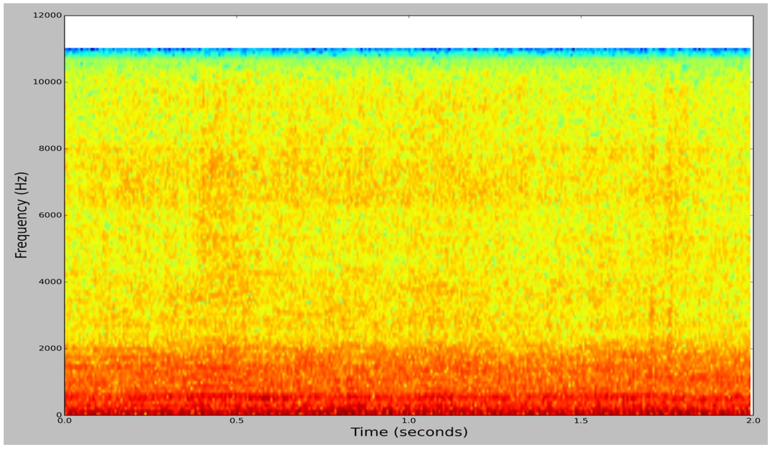
Applsci 08 01573 g001
Figure 2. Spectrogram image of a bee buzzing audio sample from BUZZ1.
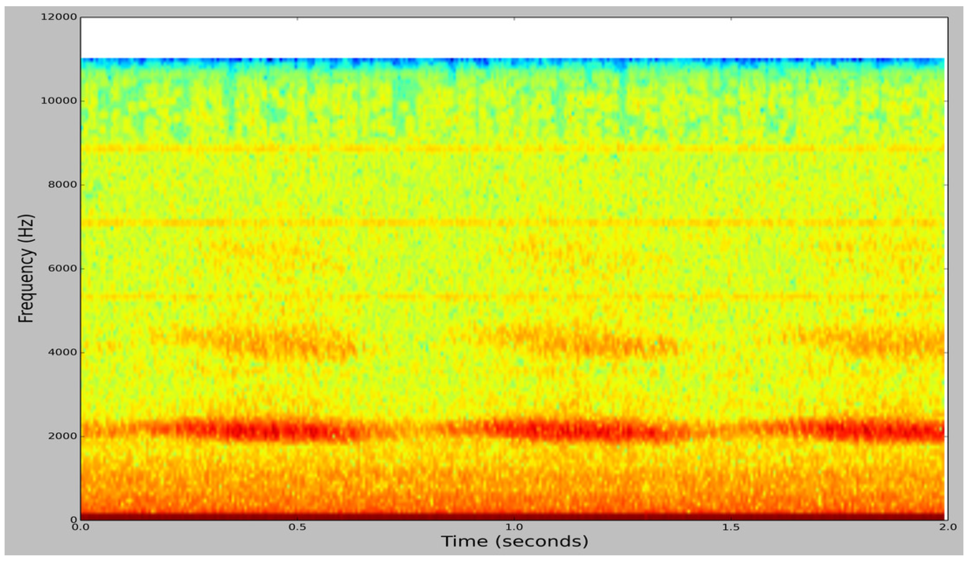
Applsci 08 01573 g002
Figure 3. Spectrogram image of a cricket chirping audio sample from BUZZ1.
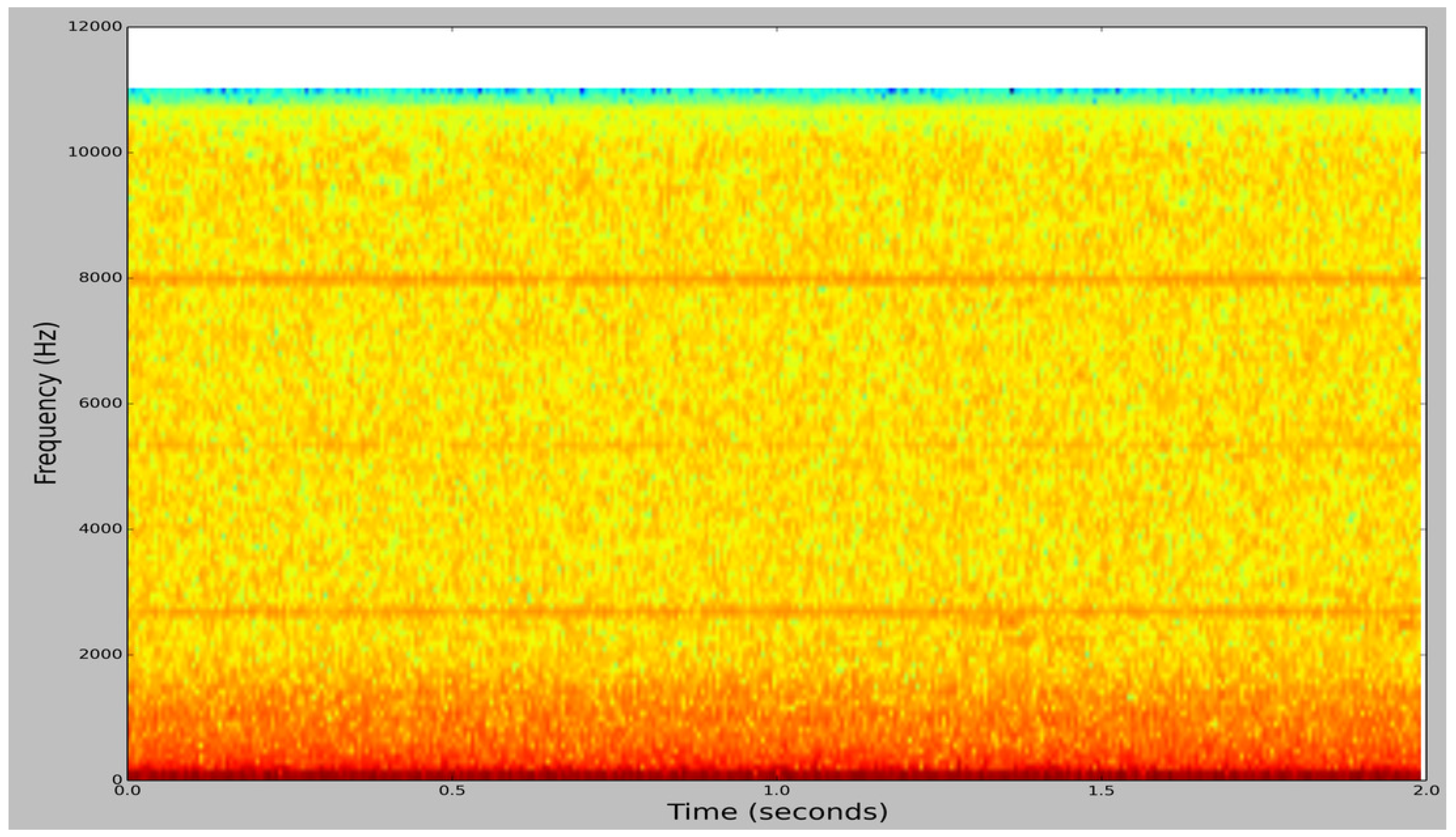
Applsci 08 01573 g003
Figure 4. Spectrogram image of an ambient noise audio sample from BUZZ1.
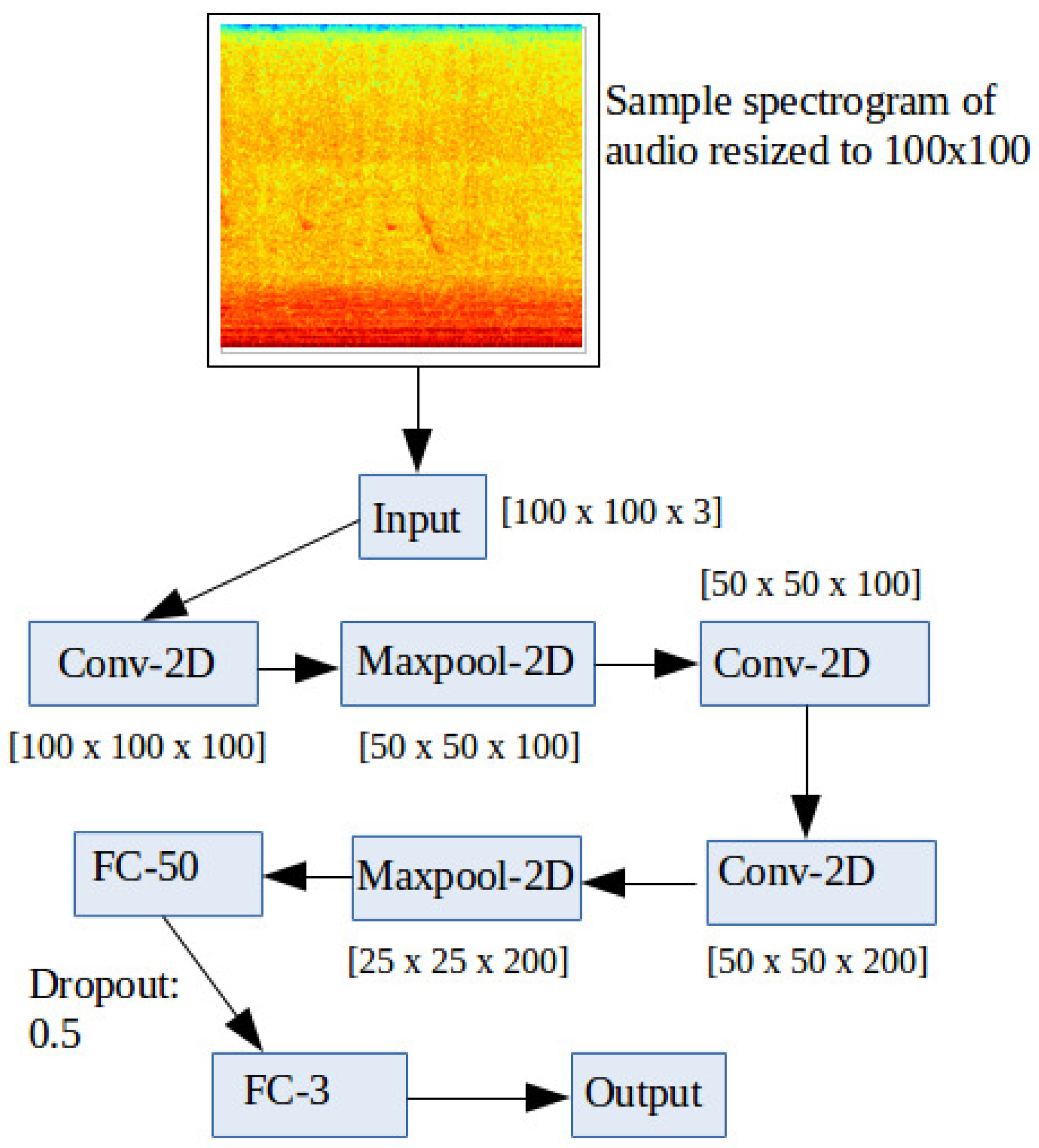
Applsci 08 01573 g004
Figure 5. SpectConvNet Architecture. The numbers below each box, except for the input, denote the dimensions of the resultant feature map following the corresponding operation in the box.
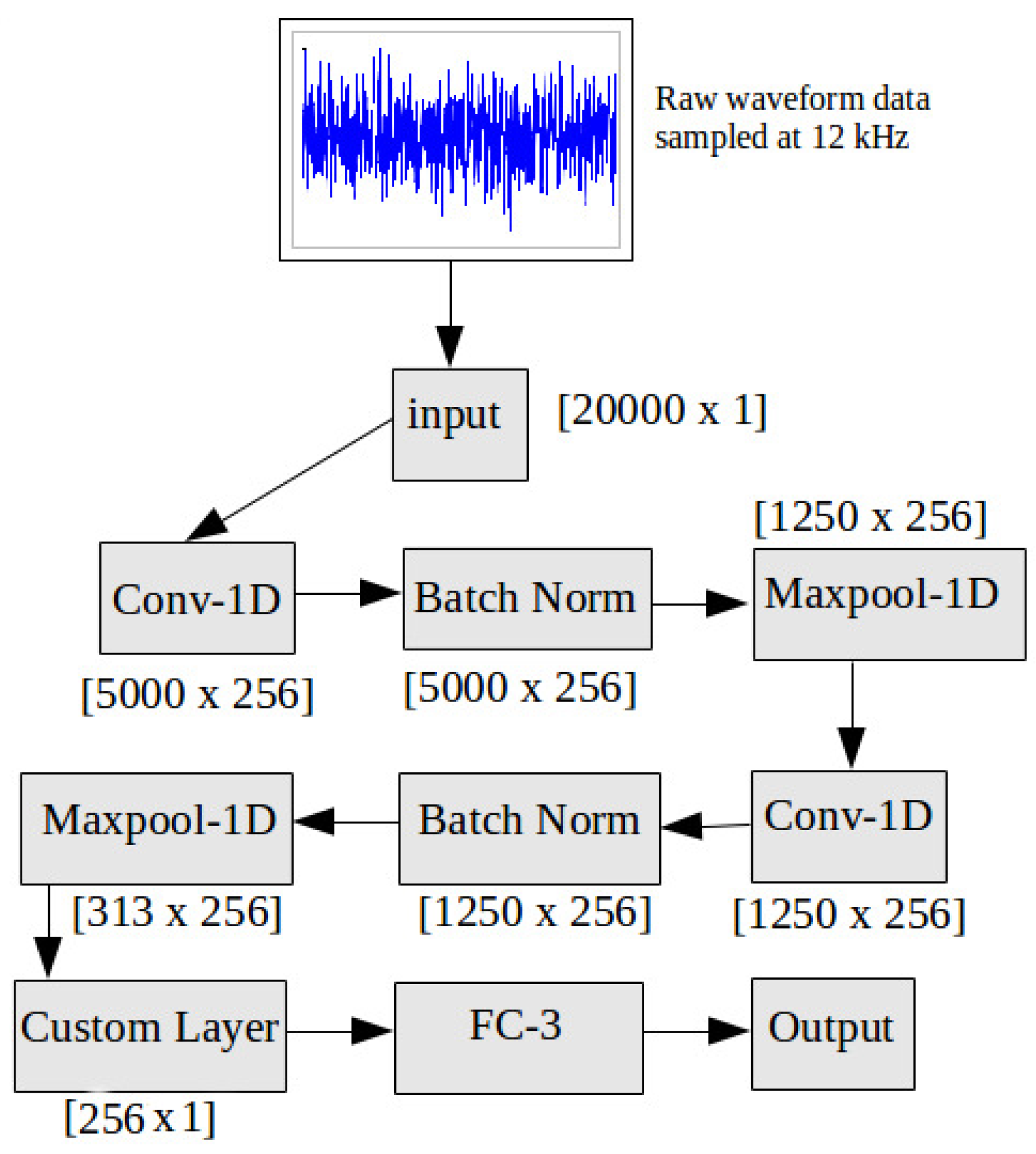
Applsci 08 01573 g005
Figure 6. SpectConvNet Control Flow. Layer by layer control flow of SpectConvNet; the numbers at the corners of each rectangle represent the corresponding dimensions.
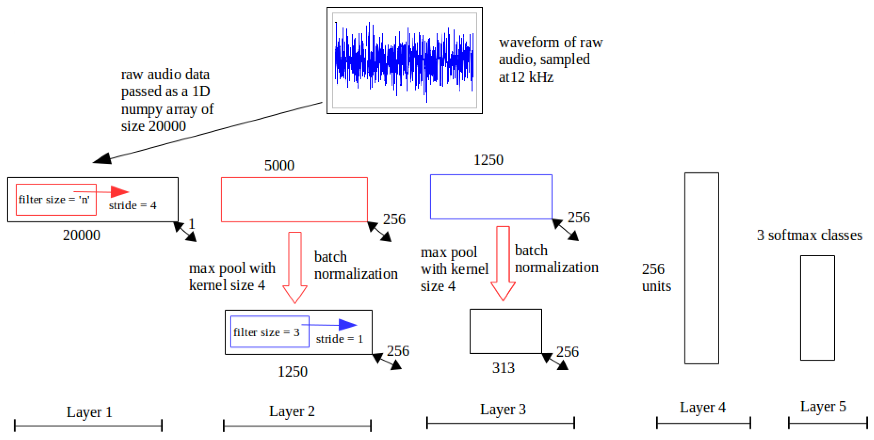
Applsci 08 01573 g006
Figure 7. RawConvNet Architecture. The numbers below each box, except for the input, are the dimensions of the resultant feature map following the corresponding operation in the box.
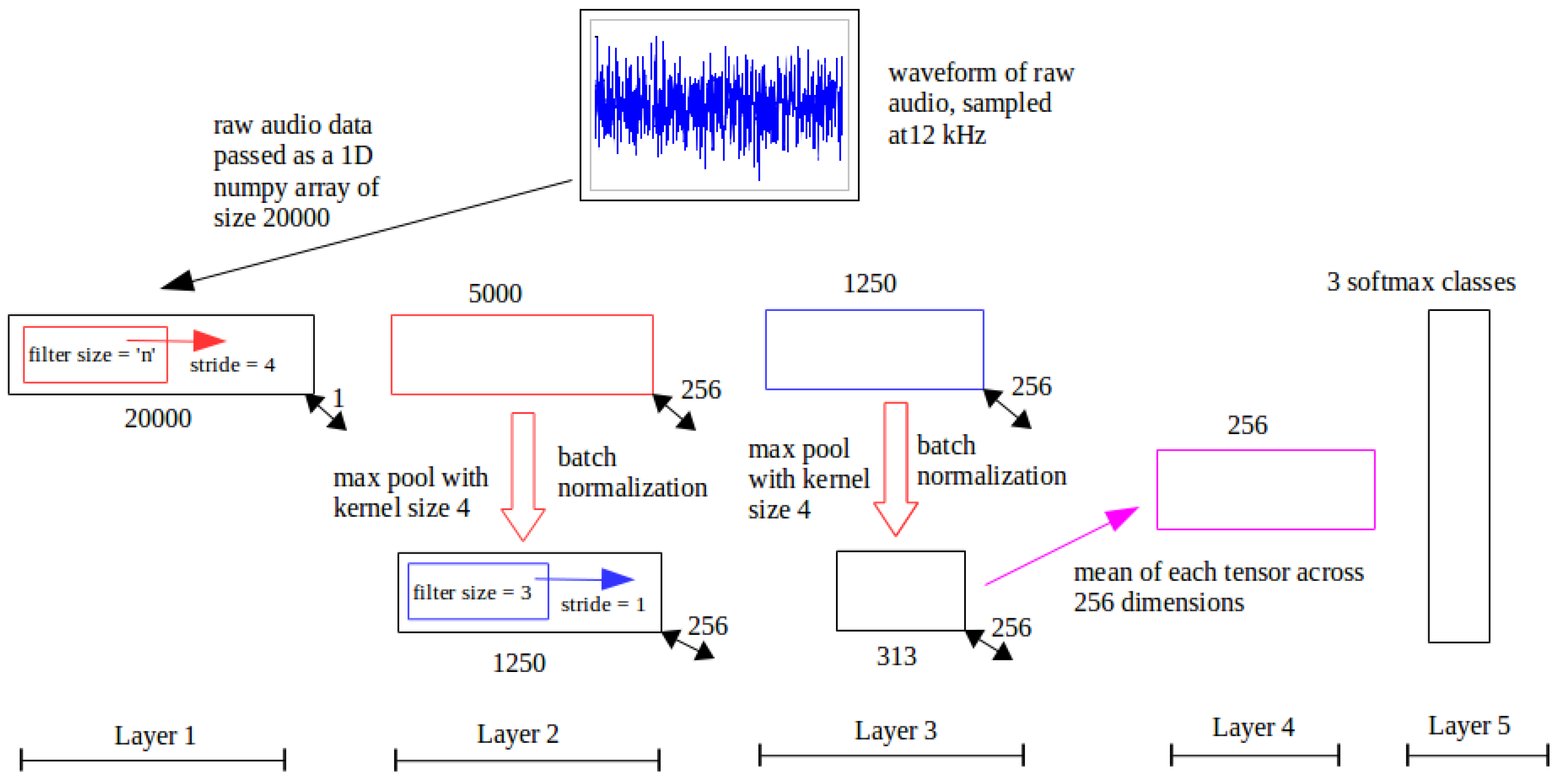
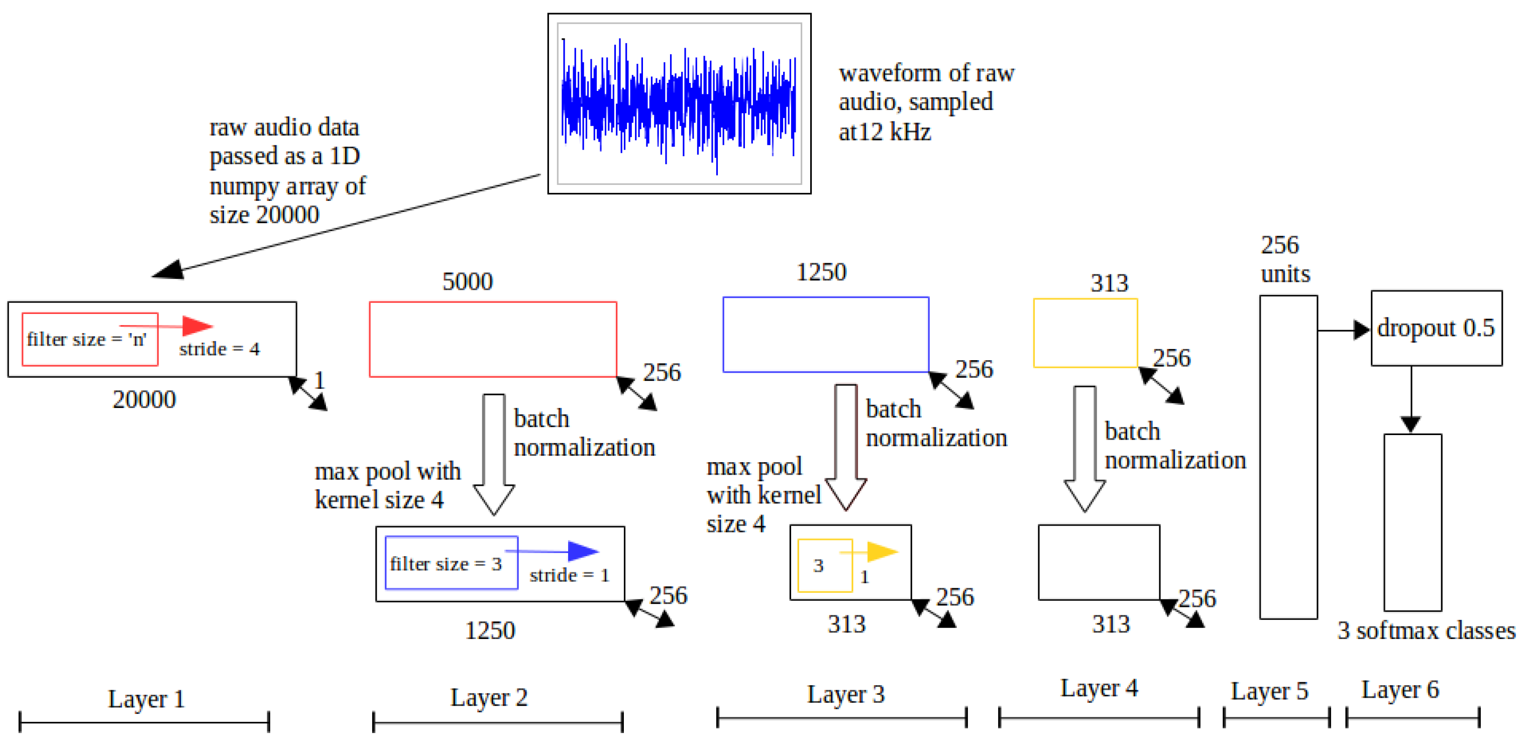
Applsci 08 01573 g007
Figure 8. RawConvNet Control Flow. Layer by layer control flow in RawConvNet trained to classify raw audio samples; the numbers below each box at the corners of each rectangle represent the corresponding dimensions; all filters and feature maps are rectangular in shape with a breadth of one unit.
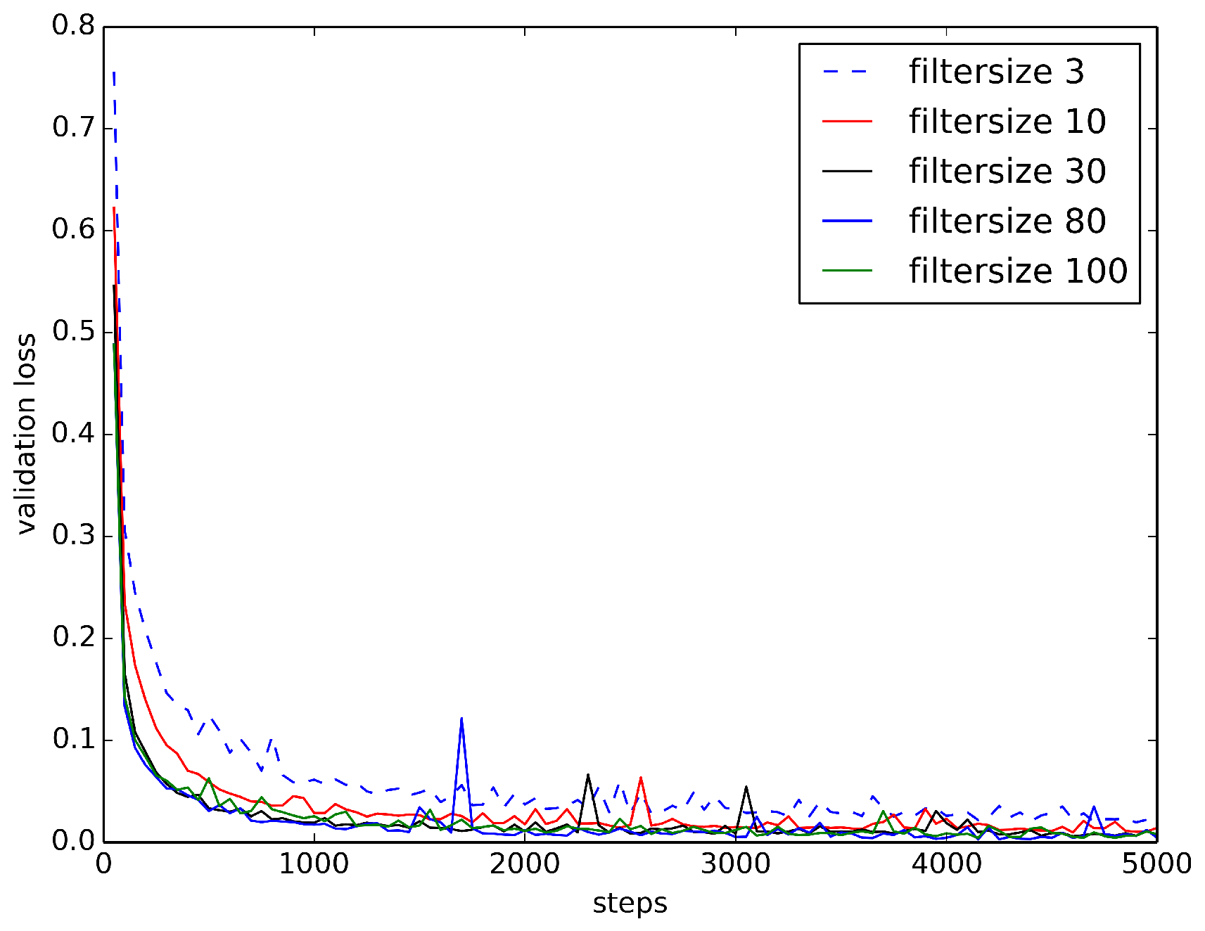
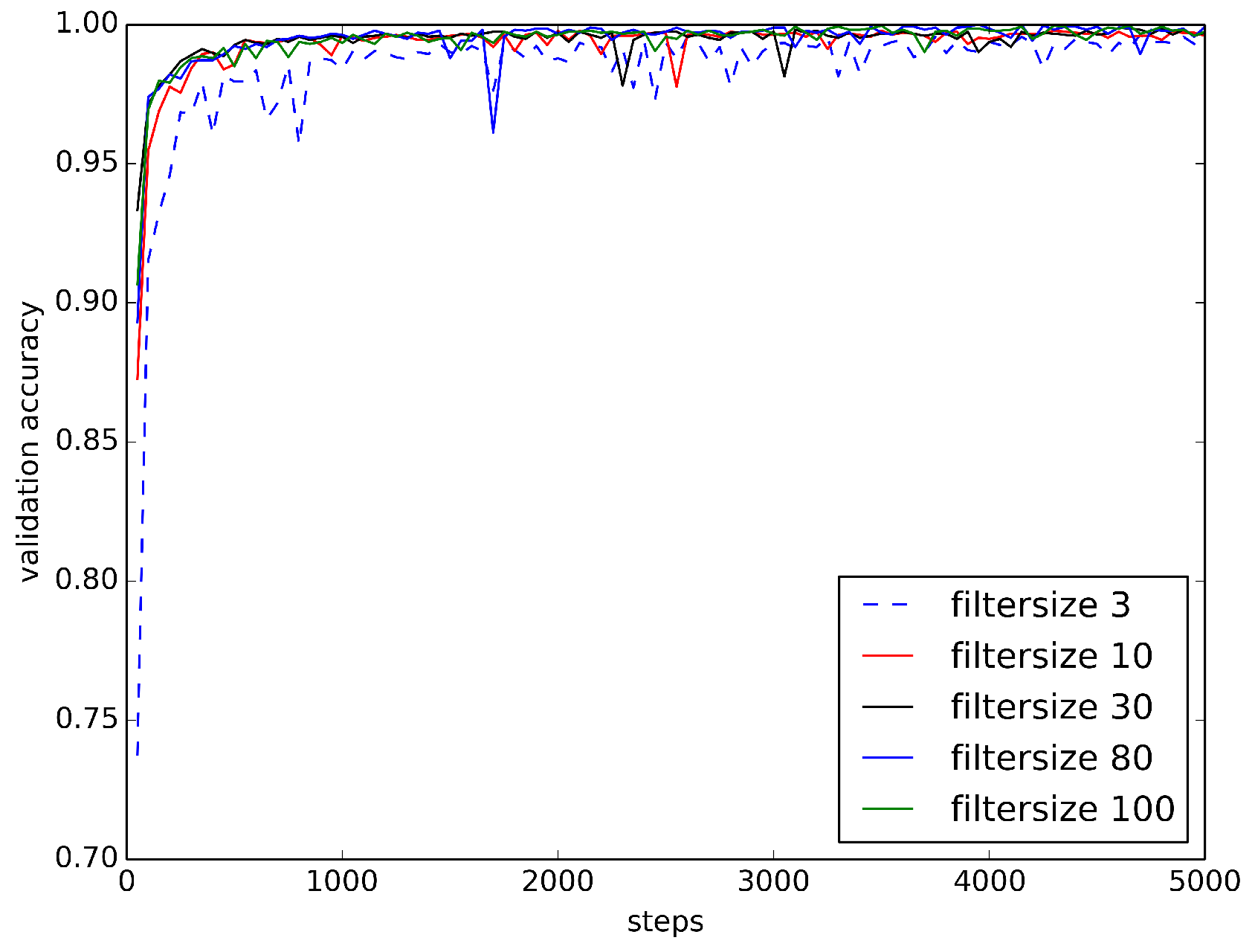
Applsci 08 01573 g008
Figure 9. Loss Curves of RawConvNet on BUZZ1 Train/Test Dataset. As the size of the receptive field increases, loss curves become smoother and decrease faster.
Applsci 08 01573 g009
Figure 10. Accuracy Curves of RawConvNet on BUZZ1 Train/Test Dataset. As the size of the receptive field increases, accuracy curves become smoother and increase faster.
Applsci 08 01573 g010
Figure 11. ConvNet 1. This ConvNet is similar to RawConvNet, but the custom layer (layer 4) of RawConvNet is replaced with an FC layer with 256 neurons.
Applsci 08 01573 g011
Figure 12. ConvNet 2. Layers 1 and 2 are identical to ConvNet 1; in layer 3, maxpooling output is convolved with 256 filters and batch normalization is used.
Applsci 08 01573 g012
Figure 13. ConvNet 3. Layers 1, 2, and 3 are identical to the same layers in ConvNet 2; in layer 4, the output is convolved with 256 filters and batch normalization is performed in layer 5.
Applsci 08 01573 g013
Table 1. SpectConvNet’s Layer Specification.
Configuration of the Best Performing Model
LayersSpecification
Layer 1Conv-2Dfilters = 100, filterSize = 3, strides = 1, activation = relu, bias = True, biasInit = zeros, weightsInit = uniform scaling, regularizer = none, weightDecay = 0.001
Layer 2Maxpool-2DkernelSize = 2, strides = none
Conv-2Dfilters = 200, filterSize = 3, strides = 1, activation = relu, bias = True, biasInit = zeros, weightsInit = uniform scaling, regularizer = none, weightDecay = 0.001
Layer 3Conv-2Dfilters = 200, filterSize = 3, strides = 1, activation = relu, bias = True, biasInit = zeros, weightsInit = uniform scaling, regularizer = none, weightDecay = 0.001
Layer 4Maxpool-2DkernelSize = 2, strides = none
Layer 5FCnumber of units = 50, activation = relu
Layer 6Dropoutkeep probability = 0.5
FCnumber of units = 3, activation = softmax
Table 2. RawConvNet’s layer specification.
LayersSpecification
Layer 1Conv-1Dfilters = 256, filterSize = n ∈ {3, 10, 30, 80, 100}, strides = 4, activation = relu, bias = True, weightsInit = xavier, biasInit = zeros, regularizer = L2, weightDecay = 0.0001
Layer 2Batch Normalizationgamma = 1.0, epsilon = 1e − 05, decay = 0.9, stddev = 0.002
Maxpool-1DkernelSize = 4, strides = none
Conv-1Dfilters = 256, filterSize = 3, strides = 1, activation = relu, bias = True, weightsInit = xavier, biasInit = zeros, regularizer = L2, weightDecay = 0.0001
Layer 3Batch Normalizationgamma = 1.0, epsilon = 1e − 05, decay = 0.9, stddev = 0.002
Maxpool-1DkernelSize = 4, strides = none
Layer 4Custom Layercalculates the mean of each feature map
Layer 5FCnumber of units = 3, activation = softmax
Table 3. SpectConvNet vs. RawConvNet on BUZZ1 train/test dataset with 70–30 train/test split. The parameter n denotes the size of the receptive field in the first layer of RawConvNet.
Number of Training Samples: 6377; Number of Testing Samples: 2733
Model NameTraining LossTraining AccuracyTesting LossTesting AccuracyRuntime per Epoch
SpectConvNet0.0061999.04%0.0070299.13%690 s
RawConvNet (n = 3)0.0275999.24%0.0304698.87%460 s
RawConvNet (n = 10)0.0136999.74%0.0142999.60%462 s
RawConvNet (n = 30)0.0082799.91%0.0067999.71%465 s
RawConvNet (n = 80)0.0069299.85%0.0043299.93%462 s
RawConvNet (n = 100)0.0045699.97%0.0078599.74%505 s
Table 4. Contribution of Custom Layer. RawConvNet is compared with ConvNets 1, 2, and 3 after 100 epochs of training with a 70–30 train/test split of the BUZZ1 train/test dataset. The receptive field size n is set to 80 for all ConvNets.
Training Samples: 6377, Testing Samples: 2733
Model NameTraining LossTraining AccuracyTesting LossTesting AccuracyRuntime per Epoch
RawConvNet0.0069299.85%0.0043299.93%462 s
ConvNet 10.5538799.77%0.5742797.59%545 s
ConvNet 20.6768668.07%0.5902298.21%532 s
ConvNet 30.6869466.81%0.5942998.02%610 s
Table 5. Classification accuracy of M1 (Logistic Regression) on BUZZ1 train/test dataset.
Test No.Test TypeScaling TypeTesting Accuracy
1train/testnone (S1)99.83%
2train/teststandard (S2)99.86%
3train/testmin max (S3)99.34%
4train/testL1 (S4)90.64%
5train/testL2 (S5)93.11%
6k-fold, k = 10none (S1)99.91%
7k-fold, k = 10standard (S2)99.89%
8k-fold, k = 10min max (S3)99.63%
9k-fold, k = 10L1 (S4)92.34%
10k-fold, k = 10L2 (S5)93.77%
Table 6. Confusion matrix for M1 (Logistic Regression) with train/test and no scaling (S1) on BUZZ1 train/test dataset with 60-40 train/test split.
TruePredicted
BeeNoiseCricketTotalTesting Accuracy
Bee117440117899.66%
Noise212430124599.83%
Cricket0012211221100%
Total Accuracy99.00%
Table 7. Confusion matrix for M1 (Logistic Regression) with train/test and L2 scaling (S5) on BUZZ1 train/test dataset with 60-40 train/test split.
TruePredicted
BeeNoiseCricketTotalTesting Accuracy
Bee117620117899.83%
Noise571038150124583.37%
Cricket4111179122196.56%
Total Accuracy93.00%
Table 8. Classification accuracy for M2 KNN on BUZZ1 train/test dataset. The accuracy is the mean accuracy computed over n ∈ [1, 25], where n is the number of nearest neighbors.
Test No.Testing TypeScaling TypeTesting Accuracy
1train/testnone (S1)99.86%
2train/teststandard (S2)99.87%
3train/testmin max (S3)99.91%
4train/testL1 (S4)99.84%
5train/testL2 (S5)99.89%
6k-fold, k = 10none (S1)99.93%
7k-fold, k = 10standard (S2)99.94%
8k-fold, k = 10min max (S3)99.96%
9k-fold, k = 10L1 (S4)99.95%
10k-fold, k = 10L2 (S5)99.96%
Table 9. Classification accuracy for M3 SVM OVR on BUZZ1 train/test dataset.
Test No.Testing TypeScaling TypeTesting Accuracy
1train/testnone (S1)99.83%
2train/teststandard (S2)99.91%
3train/testmin max (S3)99.86%
4train/testL1 (S4)91.19%
5train/testL2 (S5)93.08%
6k-fold, k = 10none (S1)99.89%
7k-fold, k = 10standard (S2)99.78%
8k-fold, k = 10min max (S3)99.67%
9k-fold, k = 10L1 (S4)92.20%
10k-fold, k = 10L2 (S5)95.06%
Table 10. Classification accuracy for M4 (Random Forests) on BUZZ1 train/test dataset.
Test No.Testing TypeScaling TypeTesting Accuracy
1train/testnone99.97%
2k-fold, k = 10none99.94%
Table 11. Confusion matrix for RawConvNet with receptive field size n = 80 on BUZZ1 validation dataset.
TruePredicted
BeeNoiseCricketTotalValidation Accuracy
Bee30000300100%
Noise7343035097.71%
Cricket04845250090.04%
Total Accuracy95.21%
Table 12. Confusion matrix for M1 (logistic regression) on BUZZ1 validation dataset.
TruePredicted
BeeNoiseCricketTotalValidation Accuracy
Bee2991030099.66%
Noise41309035095.42%
Cricket11948050096.00%
Total Accuracy94.60%
Table 13. Performance summary for DL and ML models on BUZZ1 validation dataset.
ModelValidation Accuracy
RawConvNet (n = 80)95.21%
ConvNet 1 (n = 80)74.00%
ConvNet 2 (n = 80)78.08%
ConvNet 3 (n = 80)75.04%
Logistic regression94.60%
Random forests93.21%
KNN (n = 5)85.47%
SVM OVR83.91%
Table 14. Raw audio ConvNets on BUZZ2 train/test dataset.
Training Samples: 7582, Testing Samples: 2332
Model NameTraining LossTraining AccuracyTesting LossTesting Accuracy
RawConvNet0.0034899.98%0.1425995.67%
ConvNet 10.4799799.99%0.5597694.85%
ConvNet 20.6461069.11%0.5746195.50%
ConvNet 30.6501369.62%0.5883694.64%
Table 15. Confusion matrix for logistic regression on BUZZ2 testing dataset.
TruePredicted
BeeNoiseCricketTotalTesting Accuracy
Bee673221089874.94%
Noise2932093499.78%
Cricket02647450094.80%
Total Accuracy89.15%
Table 16. Confusion matrix for KNN (n = 5) on BUZZ2 testing dataset.
TruePredicted
BeeNoiseCricketTotalTesting Accuracy
Bee8953089899.66%
Noise5929093499.46%
Cricket02647450094.80%
Total Accuracy98.54%
Table 17. Confusion matrix for SVM OVR on BUZZ2 testing dataset.
TruePredicted
BeeNoiseCricketTotalTesting Accuracy
Bee623275089869.37%
Noise9925093499.03%
Cricket2013234850069.60%
Total Accuracy81.30%
Table 18. Confusion matrix for random forests on BUZZ2 testing dataset.
TruePredicted
BeeNoiseCricketTotalTesting Accuracy
Bee8926089899.33%
Noise3931093499.67%
Cricket07043050086.00%
Total Accuracy96.61%
Table 19. Performance summary of raw audio ConvNets and ML models on BUZZ2 validation dataset.
ModelValidation Accuracy
RawConvNet (n = 80)96.53%
ConvNet 1 (n = 80)82.96%
ConvNet 2 (n = 80)83.53%
ConvNet 3 (n = 80)83.40%
Logistic regression68.53%
Random forests65.80%
KNN (n = 5)37.42%
SVM OVR56.60%
Table 20. Confusion matrix for RawConvNet with receptive field n = 80 on BUZZ2 validation dataset.
TruePredicted
BeeNoiseCricketTotalValidation Accuracy
Bee969310100096.9%
Noise69940100099.4%
Cricket067933100094.8%
Total Accuracy96.53%
Table 21. Confusion matrix for logistic regression on BUZZ2 validation dataset.
TruePredicted
BeeNoiseCricketTotalValidation Accuracy
Bee5154850100051.50%
Noise4055941100059.40%
Cricket053947100094.70%
Total Accuracy68.53%
Table 22. Confusion matrix for SpectConvNet on BUZZ2 validation dataset.
TruePredicted
BeeNoiseCricketTotalValidation Accuracy
Bee5444451100055.40%
Noise1828180100081.80%
Cricket042958100095.80%
Total Accuracy77.33%
Table 23. Summary of validation accuracies on BUZZ1 and BUZZ2 validation datasets.
ModelBUZZ1BUZZ2
RawConvNet (n = 80)95.21%96.53%
ConvNet 1 (n = 80)74.00%82.96%
ConvNet 2 (n = 80)78.08%83.53%
ConvNet 3 (n = 80)75.04%83.40%
Logistic regression94.60%68.53%
Random forests93.21%65.80%
KNN (n = 5)85.47%37.42%
SVM OVR83.91%56.60%
Table 24. Classification accuracy summary on BUZZ1 validation dataset by category.
Method vs. CategoryBeeCricketNoise
RawConvNet (n = 80)100%90.04%97.71%
ConvNet 1 (n = 80)99%90.08%28.57%
ConvNet 2 (n = 80)99%87.8%46.28%
ConvNet 3 (n = 80)100%88%35.14%
Logistic regression99.66%96%95.42%
KNN (n = 5)100%93.8%61.14%
SVM OVR100%73.8%84.57%
Random forests100%87.6%95.42%
Table 25. Classification accuracy summary on BUZZ2 validation dataset by category.
Method vs. CategoryBeeCricketNoise
RawConvNet (n = 80)96.90%94.80%99.40%
ConvNet 1 (n = 80)86.50%95.70%66.70%
ConvNet 2 (n = 80)76.60%96.40%77.60%
ConvNet 3 (n = 80)86.40%96.40%67.40%
Logistic regression51.50%94.70%59.40%
KNN (n = 5)19.40%90.80%87.20%
SVM OVR51.80%11.10%49.40%
Random forests29.20%48.80%79.80%

