Deep Learning Based Lithology Classification Using Dual-Frequency Pol-SAR Data

Abstract

Lithology classification is a crucial step in the prospecting process, and polarimetric synthetic aperture radar (Pol-SAR) imagery has been extensively used for it. However, despite significant improvements in both information content of Pol-SAR imagery and advanced classification approaches, lithology classification using Pol-SAR data may not provide satisfactory classification accuracy due to high similarity of certain classes. In this paper, a novel Pol-SAR lithology classification method based on a stacked sparse autoencoder (SSAE) is proposed. By using superpixel segmentation, new features can be extracted from dual-frequency Pol-SAR data, which can increase the class separability of the input data. Then, these features and the coherency matrices are incorporated into SSAE to classify the lithology. The classification performance is evaluated on an SIR-C dataset acquired over Xinjiang, China. The experimental result shows that this method is effective for lithology classification and can improve the overall accuracy up to 98.90%.

1. Introduction

Synthetic aperture radar (SAR) imagery has the capabilities of providing high resolution images for a large area under all-weather and all-day conditions. Therefore, it has broad applications in areas such as geological exploration, environmental monitoring, and natural disaster assessment [1]. Moreover, compared with traditional single polarized SAR images, full polarized SAR images (Pol-SAR), which contain four different Pol-SAR channels (e.g., hh, hv, vh, and vv), can provide more abundant information on land cover characteristics. It is able to provide not only the radar scattering cross section (RCS) but also the phase information of the four channels, which can reveal the scattering mechanism of targets from various aspects, such as structure and surface undulations. Hence, the classification of different lithologies based on Pol-SAR images is becoming an important tool.

In the last few decades, a variety of land cover classification algorithms have been proposed [2]. They can be broadly categorized into supervised approaches, semi-supervised approaches, and unsupervised approaches according to whether manual annotations are utilized. Kong proposed a maximum-likelihood based classification method for Pol-SAR images based on a complex Gaussian distribution [3]. This classifier was applied to single look Pol-SAR images and was modified to multi-look situations by Lee [4]. In this work, many features are extracted from Pol-SAR images, which can describe the targets from various aspects. The application of features makes it an important field in which to conduct land cover classification based on polarimetric features. For instance, Cloude and Pottier defined three features including entropy (H), anisotropy (A), and alpha ($\alpha$) by eigen decomposition. The H and $\alpha$ are widely used for classification [5]. Freeman–Durden [6] determined three-component scattering mechanisms based on physical models. In this method, double bounce, volume, and surface scattering correspond with the double-bounce scattering from a dihedral corner reflector, randomly oriented thin cylindrical dipoles, and first-order Bragg scattering, respectively. The Freeman–Durden decomposition is useful for decomposing the scattering mechanism from naturally incoherent scatterers. In Reference [7], Qi synthesized polarization decomposition, and proposed an object-based Pol-SAR image classification based on a decision tree. Through mathematical and physical analysis of Pol-SAR data, Mahdianpair presented a modified coherency matrix. The classification accuracy of wetlands was improved to 92.17% by combining the modified coherency matrix and a random forest algorithm [8].

Recently, deep learning have been proven to be very effective in classification and recognition as it can extract features automatically [9,10]. Therefore, a Pol-SAR image classification based on deep learning has attracted the attention of experts [11]. Hansch proposed the usage of complex valued neural networks for classification of different land in Pol-SAR images, which confirmed the possibility of deep learning applied to Pol-SAR image classification [12]. Lv et al. used a deep belief network as one of the deep learning models to classify different urban land covers in a Pol-SAR image [13]. In Reference [14], Zhou introduced a convolutional neural network into Pol-SAR image classification. Experimental results with Pol-SAR data indicated that the deep learning methods could provide competitive results. Xie proved the suitability of a stacked sparse autoencoder (SSAE) in the classification of Pol-SAR images [15]. However, this method is pixel-based, without considering the local spatial information. To solve this problem, Zhang et al. took all the neighborhood pixels around the cell under test as the input data, and then the Pol-SAR images were classified by SSAE [16]. This method integrated the contextual information of the neighborhood, but it has defects in practical applications especially when the target area is complex. In References [17,18], Hou and Geng proposed improved land cover classification methods based on superpixels to use the local spatial information more properly. In this study, SSAE is selected due to several advantages compared to other methods. First, unlike the convolutional neural network, SSAE is pixel-based, thus, it can classify any pixel including boundary pixels. Second, SSAE can easily handle large and multi-dimension remote sensing datasets, which is especially suitable for this study. Finally, it has a flexible and straightforward structure and has shown good results in various remote sensing applications.

In the processing of classifying different vegetation covers or different urban land covers using Pol-SAR, effective features extraction is the foundation to obtain good results. However, it is difficult to get satisfactory classification features just by using one band Pol-SAR data for lithology, since lithologies are affected by surface weathering over long periods of time, and the surface characters thus become similar among some classes [1]. To classify different lithologies, dual-frequency Pol-SAR will play a role because of the different wavelengths and varying penetrability to vegetation cover. L-frequency has the longer wavelength and better penetrability. SSAE can extract some features according to its own rules, but it cannot extract all possible features, especially those with specific physical meanings. Combining the effective handcrafted features with raw data may improve the lithology classification performance of SSAE. In this paper, new polarimetric features were proposed based on dual-frequency Pol-SAR data for the surface fluctuations of different lithologies, and then SSAE was used to extract deep features and classify different lithologies. To the best of our knowledge, this is the first attempt at the classification of lithology by combining SSAE and dual-frequency Pol-SAR data.

The paper is organized as follows: in Section 2, we explain the polarimetric features extraction and SSAE. This section also presents the new lithology classification method and describes the dataset used in the experiments. The proposed method is verified and analyzed in Section 3, at the same time, the proposed method is also compared with other methods in this section. A discussion is found in Section 4. And some useful conclusions are drawn in Section 5.

2. Materials and Methods

2.1. Pol-SAR Features Extraction

Polarimetric radar measures the complex scattering matrix of a medium with quad polarizations. The scattering matrix in the linear orthogonal polarization basis can be expressed as [19]:

$$S=\left[\begin{array}{cc}{s}_{\mathrm{hh}}& s_{\mathrm{hv}}\\ s_{\mathrm{vh}}& s_{\mathrm{vv}}\end{array}\right],$$

(1)

where $s_{\mathrm{hv}}$ is the scattering element of horizontally polarized transmitting and vertically polarized receiving waves, and the other three elements are defined similarly. In the case of reciprocal backscattering, $s_{\mathrm{vh}}=s_{\mathrm{hv}}$. The corresponding vectors $k_{\mathrm{T}}$ and $k_{\mathrm{C}}$ can be expressed by the following forms [19]:

$$k_{\mathrm{T}}=\frac{1}{\sqrt{2}}{\left[\begin{array}{ccc}{\mathrm{s}}_{\mathrm{hh}}+{\mathrm{s}}_{\mathrm{vv}}& {\mathrm{s}}_{\mathrm{hh}}-{\mathrm{s}}_{\mathrm{vv}}& 2{\mathrm{s}}_{\mathrm{hv}}\end{array}\right]}^{\mathrm{T}}$$

(2)

$$k_{\mathrm{C}}={\left[\begin{array}{ccc}{\mathrm{s}}_{\mathrm{hh}}& \sqrt{2}{\mathrm{s}}_{\mathrm{hv}}& {\mathrm{s}}_{\mathrm{vv}}\end{array}\right]}^{\mathrm{T}},$$

(3)

where ${\left[\right]}^{\mathrm{T}}$ is an ordinary transpose operation.

For the distributed targets, the $3\times 3$ coherency matrix T and covariance matrix C can be computed by [19]:

$$\begin{array}{c}T=\frac{1}{n}{\displaystyle \sum _{i=1}^n}{k}_{Ti}·k_{Ti}^H=\left[\begin{array}{ccc}{T}_{11}& T_{12}& T_{13}\\ T_{12}^{\ast }& T_{22}& T_{23}\\ T_{13}^{\ast }& T_{23}^{\ast }& T_{33}\end{array}\right]\end{array}$$

(4)

$$C=\frac{1}{n}\sum _{i=1}^n{k}_{Ci}·k_{Ci}^H=\left[\begin{array}{ccc}{C}_{11}& C_{12}& C_{13}\\ C_{12}^{\ast }& C_{22}& C_{23}\\ C_{13}^{\ast }& C_{23}^{\ast }& C_{33}\end{array}\right],$$

(5)

where ∗ stands for conjugate, and $\mathrm{H}$ denotes conjugate transpose.

Both the coherency matrix and covariance matrix contain the scattering characteristics of a distributed target. Pol-SAR data can provide characteristics of the land cover, such as permittivity, surface roughness, material, and so on. To clearly show the difference between different lithologies, some new polarimetric features should be defined and extracted based on the cross polarized ratio, co-polarized correlation coefficient, and the proportion of different scattering mechanisms, etc.

2.1.1. Cross Polarized Ratio

The cross polarized ratio is the echo ratio between the cross channel and co-polarized channels. It can be defined as follows with respect to the coherency matrix [20]:

$$r_{\mathrm{xv}}=\frac{1}{\sqrt{2}}\left|\frac{C_{22}}{C_{33}}\right|$$

(6)

$$r_{\mathrm{xh}}=\frac{1}{\sqrt{2}}\left|\frac{C_{22}}{C_{11}}\right|,$$

(7)

where $r_{\mathrm{xv}}$ and $r_{\mathrm{xh}}$ are the cross polarized ratios in vv channel and hh channel, respectively. The cross polarized ratio reflects the effect of surface roughness on scattering, which is proportional to the surface roughness, within a certain roughness range.

2.1.2. Co-Polarized Correlation Coefficient

The hh and vv channels may have different echoes due to different scattering mechanisms. The co-polarized correlation coefficient can be used to describe the scattering characters of the illuminating area, and it is defined as Equation (8) with respect to the coherency matrix [20]:

$${\rho }_{\mathrm{hh}\_\mathrm{vv}}=\frac{\left|C_{13}\right|}{\sqrt{C_{11}{C}_{33}}}.$$

(8)

The co-polarized correlation coefficient is sensitive to permittivity and surface roughness [21,22,23], which is proportional to water content when the roughness is in a certain range.

2.1.3. Freeman–Durden Decomposition

The Freeman–Durden decomposition determines three-component scattering mechanisms, including double-bounce, volume, and surface scattering, based on physical models. The Freeman decomposition is shown as follows [24]:

$$\left[C\right]=f_{\mathrm{v}}{\left[\mathrm{C}\right]}_{\mathrm{v}}+{\mathrm{f}}_{\mathrm{d}}{\left[\mathrm{C}\right]}_{\mathrm{d}}+{\mathrm{f}}_{\mathrm{s}}{\left[\mathrm{C}\right]}_{\mathrm{s}}$$

(9)

$$P_{\mathrm{v}}=\frac{8{\mathrm{f}}_{\mathrm{v}}}{3}$$

(10)

$$P_{\mathrm{d}}=f_{\mathrm{d}}\left(1+{\left|\alpha \right|}^2\right)$$

(11)

$$P_{\mathrm{s}}=f_{\mathrm{s}}\left(1+{\left|\beta \right|}^2\right),$$

(12)

where ${\left[C\right]}_{\mathrm{v}}$, ${\left[C\right]}_{\mathrm{d}}$, and ${\left[C\right]}_{\mathrm{s}}$ are the covariance matrices of the three scattering mechanisms, and $f_{\mathrm{v}}$, $f_{\mathrm{d}}$, and $f_{\mathrm{s}}$ are the scattering coefficients of double-bounce, volume, and surface, respectively. $\alpha$ and $\beta$ are the polarized coefficients of double-bounce and surface, respectively. $P_{\mathrm{v}}$, $P_{\mathrm{d}}$, and $P_{\mathrm{s}}$ are the scattering powers of the three scattering mechanisms. They can be used as features describing the scattering mechanisms because they are related to echo power from the different mechanisms.

2.2. Stacked Sparse Autoencoder

The stacked sparse autoencoder is a deep learning architecture that can extract the deep features of the input data and achieve land classification by the softmax classifier. It has been used widely in image processing and pattern recognition due to its simple process and high classification accuracy.

2.2.1. Sparse Autoencoder

A sparse autoencoder is a feedforward, fully connected, nonrecurrent neural network with an input layer, a hidden layer, and an output layer. The output layer has the same number of nodes as the input layer, and the hidden layer has more nodes than the input layer [24,25]. The sparse autoencoder self-learns so that the output get close to the input with a teacher vector identical to the input vector. This means that, the sparse autoencoder is able to extract an optimized feature set from the input data. The action of the sparse autoencoder is described as follows:

Step 1: Initialize the weight matrix and the bias vector, and calculate the outputs of the hidden layer and output layer:

$$y=f\left(W^{\left(1\right)}x+b^{\left(1\right)}\right)$$

(13)

$$\tilde{x}=g\left(W^{\left(2\right)}y+b^{\left(2\right)}\right),$$

(14)

where y and $\tilde{x}$ are the outputs of the hidden layer and output layer, respectively. $f\left(x\right)$ and $g\left(x\right)$ are the activation functions, and $f\left(x\right)=\frac{1}{1+\exp \left(-x\right)}$, $g\left(x\right)=x$. $W_{}^{\left(1\right)}$ represents the weight matrix between the input layer and the hidden layer. $W_{}^{\left(2\right)}$ is the weight matrix between the hidden layer and the output layer. $b_{}^{\left(1\right)}$ and $b_{}^{\left(2\right)}$ are the bias vectors of the hidden and output layers, respectively.

Step 2: Calculate the loss function based on outputs. The loss function used in this paper has the following form [18]:

$$J\left(W,b\right)=\frac{1}{2m}\sum _{i=1}^m{∥\tilde{x}-x∥}^2+\frac{\lambda }{2}\sum _{l=1}^2\sum _{i=1}^{s_l}\sum _{j=1}^{s_{l+1}}{\left(W_{ji}^{\left(l\right)}\right)}^2+\beta \sum _{i=1}^{s_2}KL\left(\rho ∥{\widehat{\rho }}_i\right),$$

(15)

where m is the number of training data points. $s^l$ ($l=1,2,3$) represents the number of neurons in the input layer, the hidden layer, and the output layer, respectively. The first term on the right side of Equation (15) is the traditional squared error, which stands for the difference between the output and the input. The second one is the regularization penalty which can penalize large values of the parameters to get a simpler network. This can prevent network overfitting. The third part is the sparse penalty term to improve the sparsity of the encoding representation and the Kullback–Leibler divergence $KL\left(\rho ∥{\widehat{\rho }}_i\right)$ is defined in Equation (16):

$$KL\left(\rho ∥{\widehat{\rho }}_i\right)=\rho \log \frac{\rho }{{\widehat{\rho }}_i}+\left(1-\rho \right)\log \frac{1-\rho }{1-{\widehat{\rho }}_i},$$

(16)

where ${\widehat{\rho }}_i$ is the average activation of the $i_{th}$ hidden unit over the training set. $\rho$ is the sparse parameter which is a small value close to zero. The constraint ${\widehat{\rho }}_j=\rho$ is enforced during the training. If the constraint is satisfied, the hidden activities are mostly close to zero, which ensures that the hidden layer can be forced to learn a compressed representation.

Step 3: Minimize the loss function to optimize $W^{\left(l\right)}$ and $b^{\left(l\right)}$.

It can be seen from step 2 that to get a satisfying network, we need to minimize the loss function by optimizing $W^{\left(l\right)}$ and $b^{\left(l\right)}$$(l=1,2)$. A stochastic gradient descent algorithm [26] is applied to minimize the loss function, and the process is as follow:

$$W_{}^{\left(l\right)}\leftarrow W_{}^{\left(l\right)}-\gamma \frac{\partial }{\partial W_{}^{\left(l\right)}}J\left(W,b\right)$$

(17)

$$b_{}^{\left(l\right)}\leftarrow b_{}^{\left(l\right)}-\gamma \frac{\partial }{\partial b_{}^{\left(l\right)}}J\left(W,b\right),$$

(18)

where $\gamma$ is the learning rate.

2.2.2. Stacked Sparse Autoencoder

A hierarchical training strategy is used in SSAE to construct the deep neural network to generate deep features of the input data. First, we establish several SAEs, one by one. Then train the first SAE with input features. After the first SAE is trained, regard the features obtained from the hidden layer as the input of the next SAE, for training. In this way, each SAE can be trained separately, which is called pre-training [27]. After pre-training, the decoder layers of all SAEs are removed and a softmax classifier is connected to accomplish the classification. Hence, the trained SAEs and the softmax classifier are connected to establish a whole network, which is called the SSAE. Finally, in order to obtain a more accurate classification, back-propagation is applied to adjust the parameters of the SSAE with the training samples and their labels. This step is called fine-tuning, which treats all layers of the SSAE as a single model.

After pre-training and fine-training, a trained SSAE can be obtained. We can extract optimized features from the input data to obtain favorable results in classification.

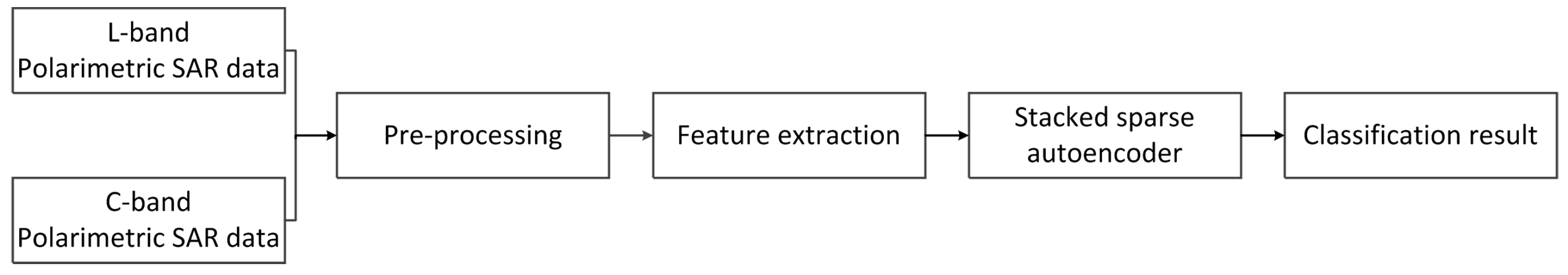
2.3. Lithology Classification Based on Deep Learning

It is challenging to classify lithology because the surface has suffered from weathering for years. In this paper, a novel classification method is proposed for lithology classification based on dual-frequency Pol-SAR data and the SSAE classifier. The proposed method has the flow chart as shown in Figure 1, which includes pre-processing of Pol-SAR data, polarimetric feature extraction, and classification with the SSAE.

2.3.1. Pol-SAR Data Pre-Processing

● Speckle Reduction

SAR images, as a consequence of their coherent nature, are subject to speckle, which decreases image quality and makes image description and interpretation difficult. Thus, a refined Lee filter [28] whose window size is $9\times 9$ is applied to the Pol-SAR dataset as a pre-processing process to reduce speckles.

● Superpixel Segmentation

A superpixel is a perceptually consistent unit with the pixels in one group being similar in character and texture. Superpixel segmentation can divide an image into a number of small contiguous regions where the pixels in each region are homogeneous. It is thus a type of oversegmentation of an image. The pixels in the same superpixel are considered as the same category in this paper.

The Pauli RGB image is formed with the intensities of three channels. After oversegmentation, the Pauli RGB image can be segmented as $\left\{I_1,\cdots ,I_N\right\}$ using the SLIC superpixel generating algorithm [29]. After segmentation, all the pixels in a superpixel will be labeled in the same class, which can be expressed by the averaged coherency matrix ${\overline{T}}_j$:

$${\overline{T}}_j=\frac{1}{n_j}\sum _{i=1}^{n_j}{T}_i,$$

(19)

where $n_j$ is the number of pixels in superpixel $I_j$.

Due to the set average processing, superpixel segmentation mitigates the influence of speckle noise compared with the original coherent matrices. To utilize the spatial features of Pol-SAR data, the polarimetric features used in the novel classification are all extracted from the superpixel segmented image.

2.3.2. Lithology Feature Extraction

Despite using advanced remote sensing tools, classification of lithology is challenging due to high similarity caused by weathering and coverage, which can produce confusion in the classification. Thus, in this study, we extract new features to increase the separability among different classes and to improve the classifier performance.

The volume and surface scattering power obtained from Freeman decomposition is used in this study to indicate the differences in structures. The cross polarized ratio measures the roughness of the surface, and the co-polarized correlation coefficient is related to the permittivity. The lithology can be well characterized by combining these features. The lithological differences are sensitive to the wavelength of electromagnetic waves. Therefore, we can improve the classifier by synthesizing different frequency Pol-SAR data. New features are defined in this paper based on the cross polarized ratio, co-polarized correlation coefficient, and the Freeman–Durden decomposition to indicate how features change with different wavelengths:

$$\Delta r_{\mathrm{xv}}=\frac{r_{\mathrm{xv}\_\mathrm{C}}-r_{\mathrm{xv}\_\mathrm{L}}}{r_{\mathrm{xv}\_\mathrm{C}}+r_{\mathrm{xv}\_\mathrm{L}}}$$

(20)

$$\Delta \rho =\frac{{\rho }_{\_\mathrm{C}}-{\rho }_{\_\mathrm{L}}}{{\rho }_{\_\mathrm{L}}+{\rho }_{\_\mathrm{C}}}$$

(21)

$$\Delta P_{\mathrm{v}}=\frac{P_{\mathrm{v}\_\mathrm{C}}-P_{\mathrm{v}\_\mathrm{L}}}{P_{\mathrm{v}\_\mathrm{C}}+P_{\mathrm{v}\_\mathrm{L}}}$$

(22)

$$\Delta P_{\mathrm{s}}=\frac{P_{\mathrm{s}\_\mathrm{C}}-P_{\mathrm{s}\_\mathrm{L}}}{P_{\mathrm{s}\_\mathrm{L}}+P_{\mathrm{s}\_\mathrm{C}}},$$

(23)

where $r_{\mathrm{xv}\_\mathrm{i}}$, ${\rho }_{\_i}$, and $P_{\mathrm{v}\_\mathrm{i}}$ and $P_{\mathrm{s}\_\mathrm{i}}$$\left(i=\mathrm{L},\mathrm{C}\right)$ are the cross polarized ratio, co-polarized correlation coefficient, and volume and surface scattering powers under L and C bands. Equations (20)–(23) represent the trend and variation of the target characteristics when the imaging frequency changes. This indicates the differences in the lithology scattering mechanisms. Scattering mechanisms corresponding to target feature variations are shown in

Table 1. Scattering mechanisms corresponding to target feature variations.

Features Variation ($\mathbf{C}\to \mathbf{L}$)	$>0$	$<0$
$\Delta r_{\mathrm{xv}}$	Increased surface roughness	Decreased surface roughness
$\Delta \rho$	Increased permittivity	Decreased permittivity
$\Delta P_{\mathrm{v}}$	Increased volume scattering	Decreased volume scattering
$\Delta P_{\mathrm{s}}$	Increased surface scattering	Decreased surface scattering

. Compared with the single-frequency Pol-SAR image classification, the proposed method based on dual-frequency Pol-SAR images exploits the trend and variation of the features with frequency change rather than static and isolated scattering mechanisms.

Therefore, the new classification feature vector is constructed, including $T_{11\_i}$, $real\left(T_{12\_i}\right)$, $imag\left(T_{12\_i}\right)$, $real\left(T_{13\_i}\right)$, $imag\left(T_{12\_i}\right)$, $T_{22\_i}$, $real\left(T_{23\_i}\right)$, $imag\left(T_{23\_i}\right)$, $T_{33\_i}$, ($i=\mathrm{L},\mathrm{C}$), $\Delta r_{\mathrm{xv}}$, $\Delta \rho$, $\Delta P_{\mathrm{v}}$, and $\Delta P_{\mathrm{s}}$, which is utilized to distinguish different lithology.

2.3.3. Lithology Classification

In this paper, SSAE is used to classify the lithology. Every pixel in the Pol-SAR image can be used for feature vector extraction. Then, we determine an optimal configuration of SSAE according to the classification results. The determined SSAE can be trained by the training dataset. Finally, lithologies can be classified by the trained SSAE.

The optimal architecture of SSAE can be obtained if the number of hidden layers and neurons of each layer are fixed. The steps are as follows.

Step 1: Determine the optimal number of layers. The dataset is used for training on different SSAE topologies with increasing depth but the same neurons. The classification accuracy is analyzed to compare different architectures. In this way, we can obtain the SSAE with most suitable number of layers for this dataset.

Step 2: Determine the suitable number of neurons in each hidden layer. tTe dataset is used for training on different SSAEs. The number of hidden layers in each SSAE has been determined by step 1, and here the number of neurons is varying. Then we can obtain the optimal number of neurons by evaluating the classification accuracy of these SSAEs.

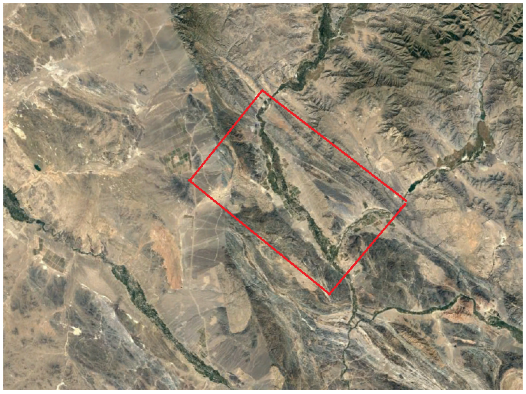
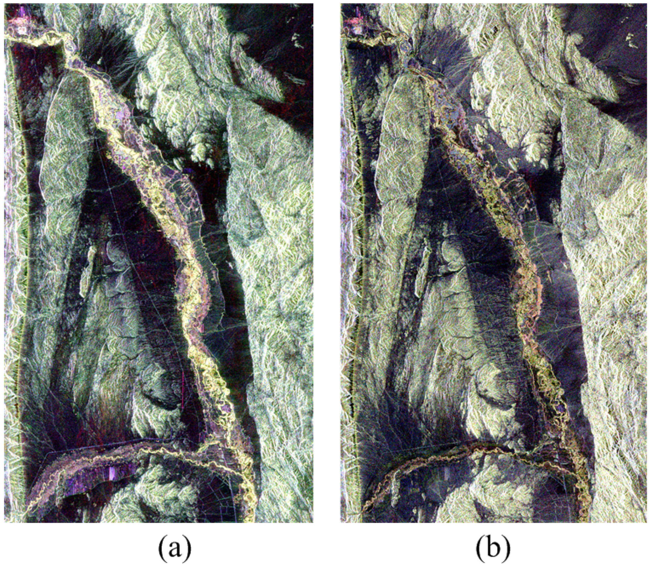
2.4. Dataset Description

The experimental data used in this paper are acquired by the NASA/JPL SIR-C system in Qinghe Xinjiang, China, in 1994, including the 4-Look Complex L-Band and C-Band datasets with a resolution of 12.5 m × 12.5 m. According to the ground truth acquired by the Chinese Academy of Sciences in 1994, there are eight classes of lithology in the experimental area, including Alluvium (${\mathrm{Q}}_4^{\mathrm{a}1}$), Diluvium (${\mathrm{Q}}_{2-3}^{\mathrm{p}1}$), Alluvium–Diluvium (${\mathrm{Q}}_{3-4}^{\mathrm{a}\mathrm{p}1}$), Beitashan Formation (${\mathrm{D}}_{2\mathrm{b}}$), Biotite granite, Leucogranite (${\gamma }_4^{2\mathrm{c}}$), Upper Aermantie Formation (${\mathrm{D}}_{3\mathrm{a}}^{\mathrm{b}}$), Nanmingshui Formation (${\mathrm{C}}_{1\mathrm{n}}$), and Mayinebo Formation (${\mathrm{D}}_{1\mathrm{m}}$). The reference map of this area is provided in Figure 2. The L-Band and C-Band Pauli RGB images are shown in Figure 3. Figure 4 is the ground truth where black color means that the pixels have no class labels.

3. Results

In this section, the performance of the proposed method is verified and analyzed.

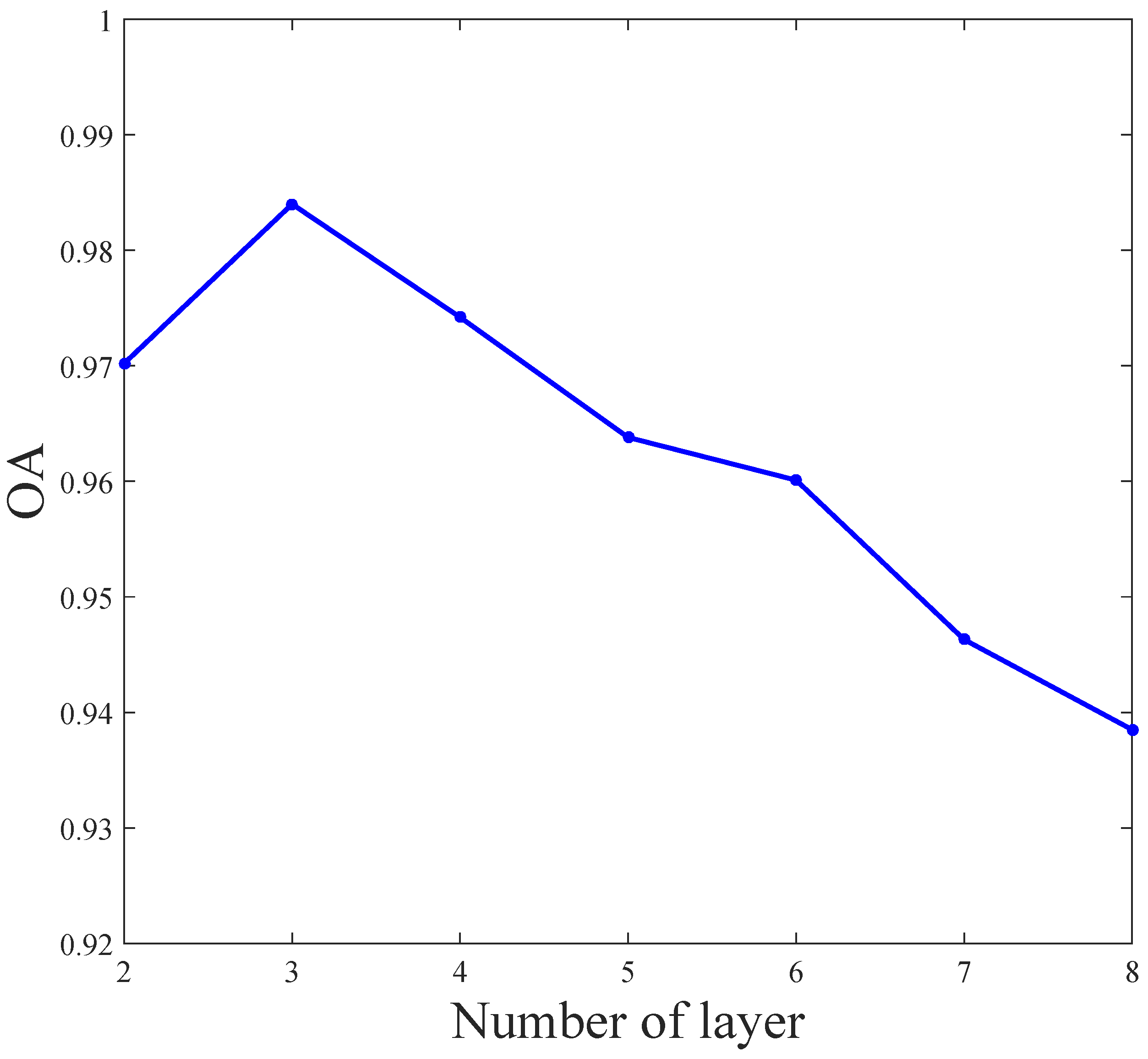
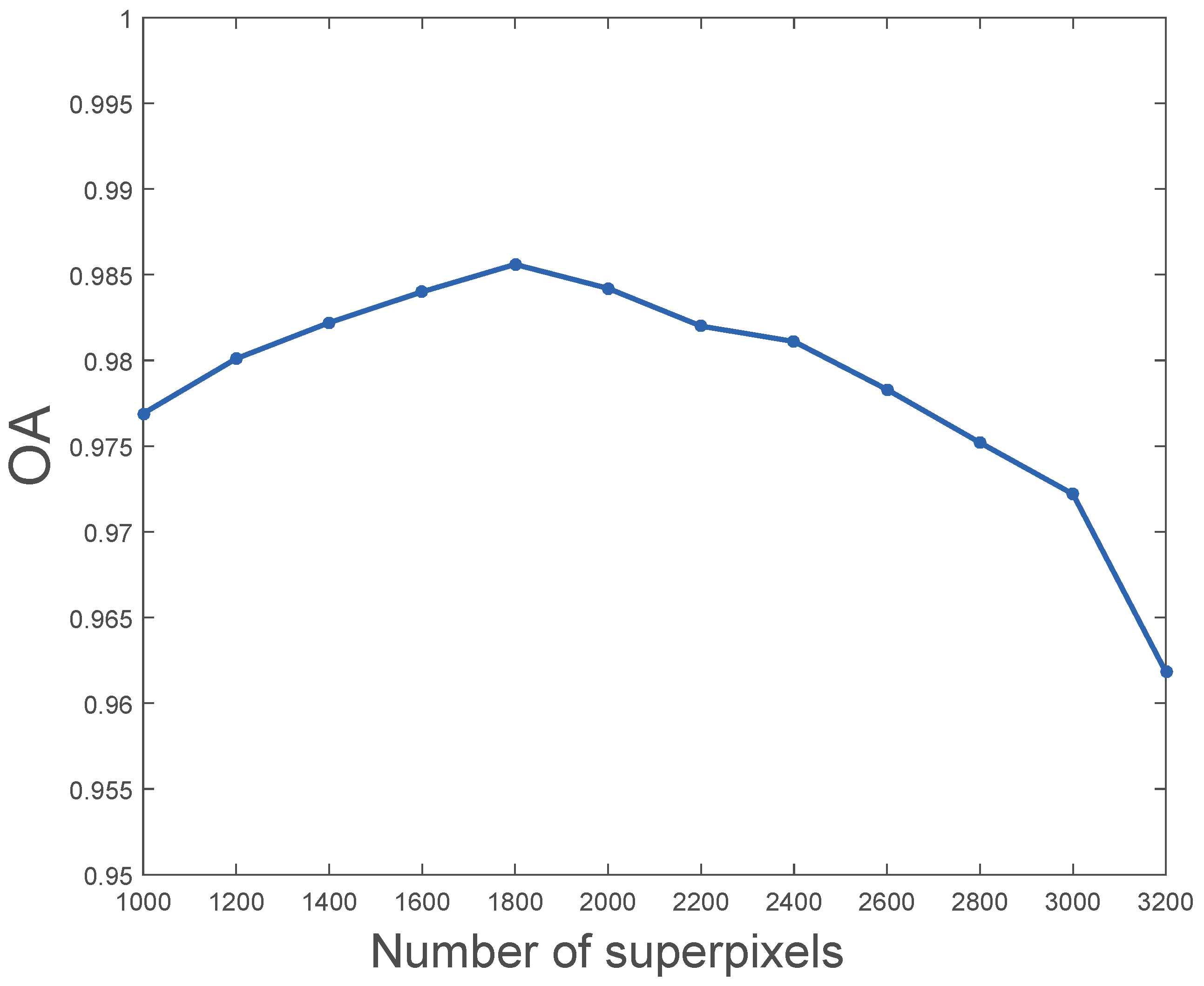
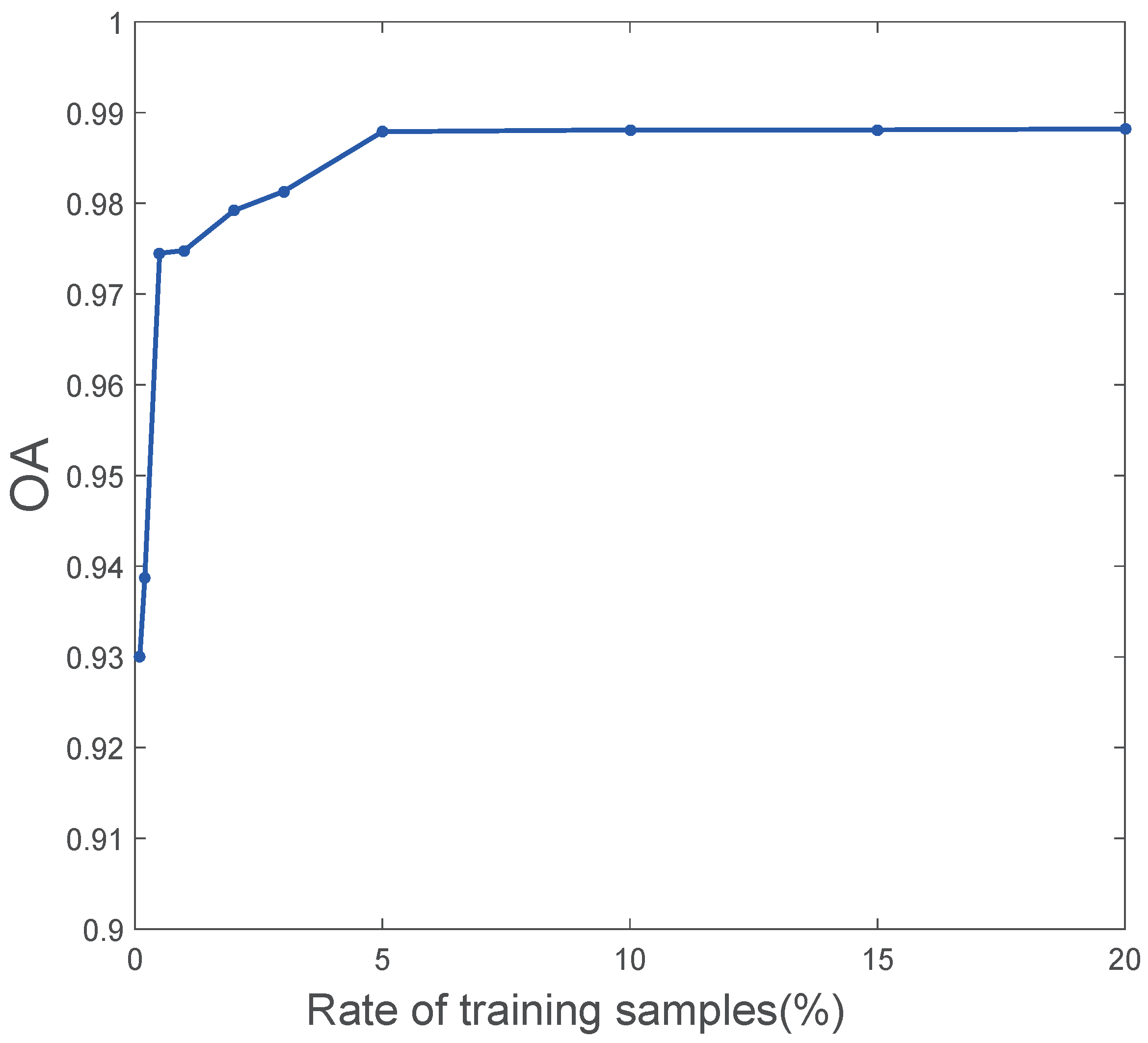
3.1. Experimental Parameters

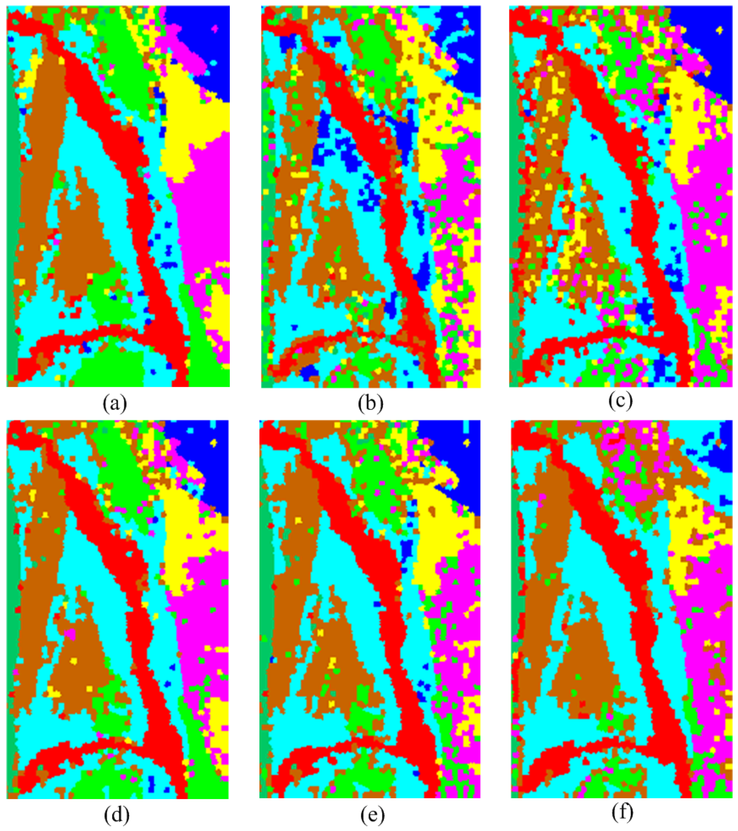
Our algorithm comes with some parameters that can affect the classification performance, such as the number of hidden layers and nodes in the SSAE, and the number of superpixels and training pixels. Specifically, the number of hidden layers and nodes in each layer can influence the performance of the SSAE. Moreover, superpixels divided from the Pauli RGB image can affect the classification results. A smaller number of superpixels implies that a superpixel contains more pixels and therefore more contextual information of the neighborhood can be considered. However, the classification of boundaries becomes poor when the number of superpixels is too small. Furthermore, the number of training pixels also influences the estimation accuracy. In order to analyze the impact of these parameters, experiments are carried out with the Qinghe dataset.

To determine the optimal number of layers, SSAE topologies with increasing depth were trained with the same number of superpixels and training pixels. In this experiment, the SIR-C image was divided into 2200 superpixels, and 10% of labeled pixels were randomly selected as the training set to train the network. The overall accuracy (OA), which is defined in Equation (24), is calculated to compare different architectures. From the plot shown in Figure 5, it can be seen that a three-layer SSAE is the most suitable for the dataset. Furthermore, the network has 60, 80 ,and 100 nodes in these hidden layers. From the above mentioned results, a three-layer SSAE with 60, 80, and 100 nodes was applied in the following experiments. The OA is:

$$OA=\frac{{\displaystyle \sum _{i=1}^r}{x}_{ii}}{N},$$

(24)

where N is the number of total samples, r denotes the number of classes, and $x_{ii}$ is the diagonal elements in the confusion matrix.

Then, the optimal number of superpixels obtained from the SIR-C image can be determined by following experiments. In this step, the SIR-C image is divided into 1000, 1200, 1400, 1600, 1800, 2000, 2200, 2400, 2600, 2800, 3000, and 3200 superpixels, and then classification performance is analyzed to find the optimal number of superpixels. As shown in Figure 6, 1800 superpixels is the favorable parameter.

Finally, we validate the performance of our network architecture with different numbers of training pixels. We respectively choose 0.1%, 0.2%, 0.5%, 1%, 2% , 3%, 5%, 10%, 15%, and 20% of labeled pixels as the training set to train the network. From Figure 7, we find that, when the rate of training samples increases from 0.1% to 5%, the OA of classification increases sharply at first, and then a stable and high OA is obtained. 5% of the labeled pixels is enough to train the network, and it can prevent overfitting. Thus, as shown in

Table 2. Training and testing pixel numbers for the Qinghe dataset.

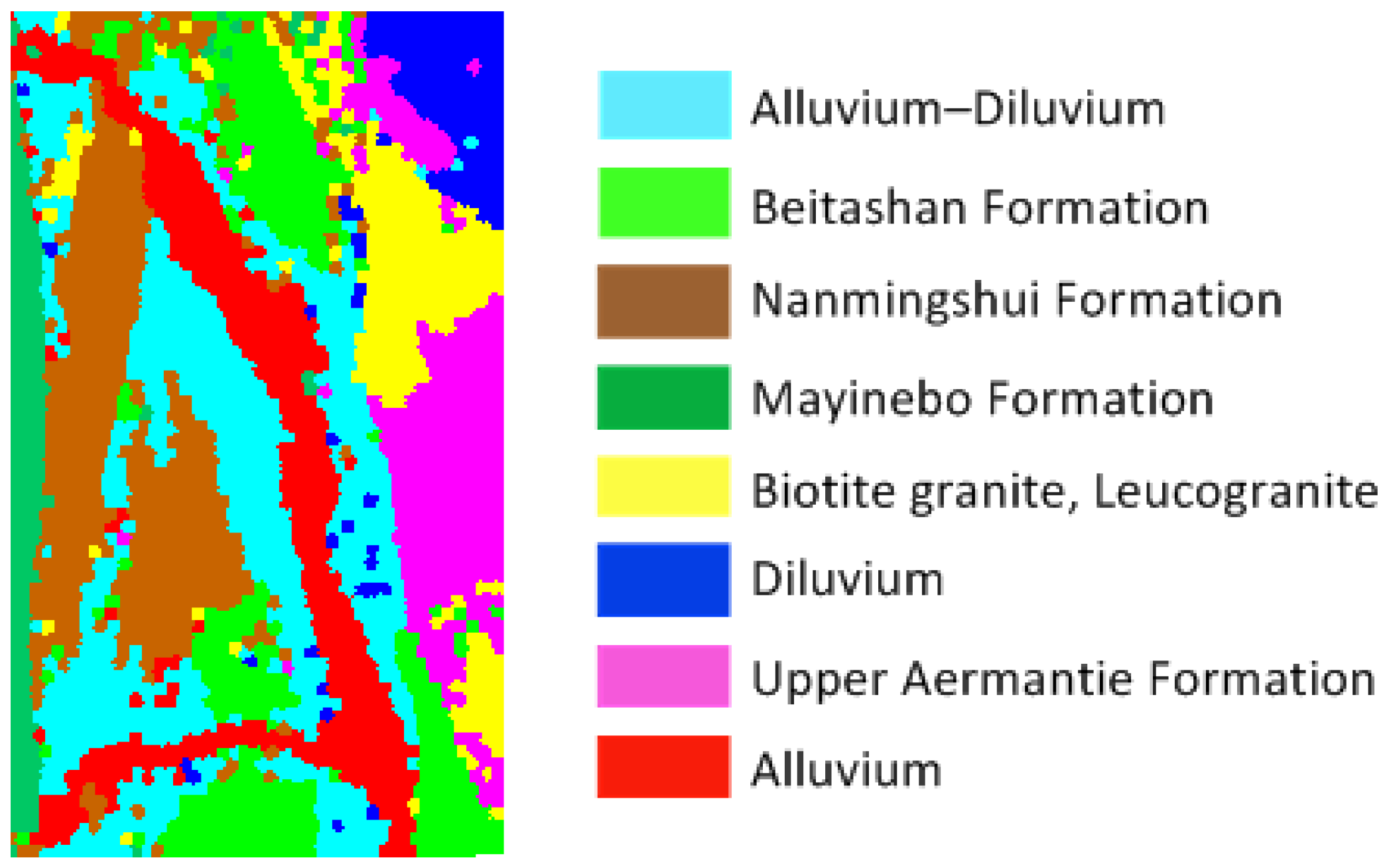
	Class Label	All Pixels	Training Pixels	Testing Pixels
Alluvium	1	343,987	17,199	326,788
Beitashan Formation	2	322,833	16,142	306,691
Diluvium	3	167,735	8,387	159,348
Biotite granite, Leucogranite	4	211,923	10,596	201,327
Upper Aermantie Formation	5	318,968	15,948	303,020
Alluvium–Diluvium	6	371,692	18,585	353,107
Nanmingshui Formation	7	352,351	17,618	334,733
Mayinebo Formation	8	212,628	10,631	208,375
Total	-	2,302,117	115,106	2,187,011

, 5% of the labeled pixels are randomly selected as a training dataset, and the remainder are regarded as the testing dataset.

3.2. Classification Results

In this experiment, using the proposed method, the Pol-SAR images can be classified.

First, the data should be pre-processed. A refined Lee filter with 9 × 9 window size is chosen to reduce the noise. Then, after superpixel segmentation, 1800 superpixels remain, and the result is shown in Figure 8. It can be seen that most pixels belonging to the same superpixel have nearly the same color. This means that these pixels have nearly the same scattering mechanism, and can be classified as one group.

Then, polarimetric features can be extracted from the Pol-SAR data, and the features maps are shown in Figure 9. It can be seen that when just using the original features, some classes can not be distinguished, however significant differences can be found in the features maps between these two classes when the new features are used.

Finally, extracted features are entered into the SSAE which has three hidden layers with 60, 80, and 100 nodes, respectively. The classified map is depicted in Figure 10.

To varify the advantages of the new features compared to the original features (${\mathrm{P}}_{\mathrm{s}\_\mathrm{i}}$, ${\mathrm{P}}_{\mathrm{v}\_\mathrm{i}}$, ${\rho }_{\mathrm{hh}\_\mathrm{vv}\_\mathrm{i}}$, and $r_{\mathrm{xv}\_\mathrm{i}}$ (i = L, C)), comparison experiments and analysis are conducted. In this experiment, we use $d_{i,j}$, which is defined as follows, to describe the difference between class i and j:

$$d_{i,j}=\max \left\{\frac{{\overline{f}}_i}{{\overline{f}}_j},\frac{{\overline{f}}_j}{{\overline{f}}_i}\right\},$$

(25)

where ${\overline{f}}_i$ and ${\overline{f}}_j$ represent the average of class i and j with feature f, respectively. $d_{i,j}$ is a number greater than 1, and it is proportional to the difference between two classes.

From Figure 3 and Figure 4, we can directly see that Beitashan Formation (class 2) and Upper Aermantie Formation (class 5) are difficult to distinguish, Diluvium (class 3) is easily confused with Alluvium–Diluvium (class 6). Therefore, $d_{2,5}$ and $d_{3,6}$ are calculated in the regions marked in Figure 9a with original features and new features.

As can be seen in

Table 3. The difference between two classes.

	${\mathbf{P}}_{\mathbf{s}\_\mathbf{L}}$	${\mathbf{P}}_{\mathbf{s}\_\mathbf{C}}$	$\mathbf{\Delta }{\mathbf{P}}_{\mathbf{s}}$	${\mathbf{P}}_{\mathbf{v}\_\mathbf{L}}$	${\mathbf{P}}_{\mathbf{v}\_\mathbf{C}}$	$\mathbf{\Delta }{\mathbf{P}}_{\mathbf{v}}$	${\mathit{\rho }}_{\_\mathbf{C}}$	${\mathit{\rho }}_{\_\mathbf{L}}$	$\mathbf{\Delta }\mathit{\rho }$	${\mathit{r}}_{\mathbf{xv}\_\mathbf{C}}$	${\mathit{r}}_{\mathbf{xv}\_\mathbf{L}}$	$\mathbf{\Delta }{\mathit{r}}_{\mathbf{xv}}$
$d_{2,5}$	1.08	1.06	1.26	1.03	1.08	1.21	1.01	1.03	1.20	1.02	1.06	1.31
$d_{3,6}$	1.00	1.03	1.10	1.02	1.15	1.18	1.01	1.01	1.04	1.03	1.11	1.27

, $d_{2,5}$ and $d_{3,6}$ for the new features are greater than those for the original features, which indicates that the new features are more effective in increasing the class separability than the original features. For example, for the situation that just uses $r_{xv\_L}$, $d_{3,6}$ is 1.06. However, $d_{3,6}$ is improved to 1.31 when $\Delta r_{xv}$ is used.

As shown in Figure 10, the proposed method can generate competitive visual effects with good connectivity and smooth borders, compared with the ground truth. Thus, lithology can be classified in a good way with this method.

Although favorable results of lithology classification can be obtained with the proposed method, several different classes of lithology are confused. The confusion matrix is shown in

Table 4. Confusion Matrix.

	Predicted	Class 1	Class 2	Class 3	Class 4	Class 5	Class 6	Class 7	Class 8
Real
Class 1		306,036	0	155	0	187	1,767	1,413	30
Class 2		205	286,749	0	21	889	3	2,682	0
Class 3		0	0	147,703	60	0	3,198	0	0
Class 4		0	0	49	189,009	1,436	28	208	0
Class 5		0	191	795	307	285,751	27	0	0
Class 6		0	18	6,420	0	221	327,856	7	0
Class 7		0	0	0	204	0	406	316,459	46
Class 8		0	0	0	0	0	38	83	119,343

.

The Diluvium is mostly confused with Alluvium–Diluvium, leading to a low classification accuracy of these classes. This is primarily due to the fact that both Diluvium and Alluvium–Diluvium have a low back-scattering power.

3.3. Comparison with Other Classifiers

To validate and test the performance of the proposed method, the SIR-C data of Qinghe Xinjiang, China, was used. The experimental verification included two aspects, which are the classification accuracy and computational burden.

3.3.1. Classification Accuracy

To validate the lithology classification accuracy, a comparison between the proposed method and other methods is made in this section. The classifiers compared are three SSAE methods with different inputs, the Support Vector Machine (SVM) classifier, and Hou’s method from Reference [18]. The three SSAE methods in this paper can be labeled as M1, M2, and M3, whose inputs are the coherency matrix of the L-frequency, the C-frequency, and the dual-frequency Pol-SAR data, respectively. Both the SVM classifier and Hou’s method utilized the same features as the proposed method. The superpixel segmentation is introduced for these comparison methods. The SVM is a typical method in classification and Hou’s method is a state of the art method in Pol-SAR image classification. In the experiment of SVM, ’rbf’ is used as the kernel and c = 100, gamma = 0.01. The classification accuracy is reported in

Table 5. Classification accuracy.

	The Proposed Method	M1	M2	M3	SVM	Hou’s Method
Class 1	0.9885	0.9154	0.9719	0.9863	0.9813	0.9885
Class 2	0.9869	0.5497	0.5754	0.9450	0.7250	0.5475
Class 3	0.9784	0.7628	0.9982	0.9439	0.9640	0.9578
Class 4	0.9910	0.7912	0.7147	0.8716	0.8185	0.8772
Class 5	0.9954	0.6190	0.8800	0.9121	0.7145	0.6922
Class 6	0.9801	0.6843	0.8690	0.9743	0.9443	0.8744
Class 7	0.9979	0.8295	0.7000	0.9514	0.9155	0.8227
Class 8	0.9990	0.6772	0.8141	0.9446	0.8910	0.6680
OA	0.9890	0.7299	0.8055	0.9470	0.8669	0.8005
Kappa	0.9873	0.6884	0.7742	0.9385	0.8458	0.7704

and the results are plotted in Figure 11. The OA and kappa coefficient (Kappa) are calculated to evaluate the classification performance. Kappa is defined as:

$$\mathrm{Kappa}=\frac{N{\displaystyle \sum _{i=1}^r}{x}_{ii}-{\displaystyle \sum _{i=1}^r}\left(x_{i+}\times x_{+i}\right)}{N^2-{\displaystyle \sum _{i=1}^r}\left(x_{i+}\times x_{+i}\right)},$$

(26)

where N is the number of total samples, r denotes the number of classes, $x_{ii}$ is the diagonal elements in confusion matrix, and $x_{i+}$ and $x_{+i}$ are the number of samples in the ith row and the ith column of confusion matrix, respectively.

It can be directly seen from Figure 11 that the classification performance is improved significantly compared with the other five methods. As shown in Table 5, the proposed method has a lithology classification accuracy of 98.90% in this experiment, and it outperforms M1, M2, M3, SVM, and Hou’s method, which have accuracies of 72.99%, 80.55%, 94.70%, 86.69%, and 80.05%, respectively. The classification accuracy of lithology, especially for classes with high similarity, has been improved with the proposed method. From the results of M1, M2, and M3, we can conclude that dual-frequency Pol-SAR data can provide more information than single frequency Pol-SAR data; the accuracy of M3 is better than M1 and M2. As can be seen from the classification accuracy of the proposed method and M3, the new features extracted from dual-frequency Pol-SAR data are effective and can improve the classification accuracy of lithology. SSAE is more suitable for lithology classification than SVM, because SSAE can extract deep features of input data and classify the lithology with these features. Therefore, the classification result of the proposed method is better than SVM. By comparing the performance of the proposed method and Hou’s method, we can tell that the algorithm in this paper is more effective for lithology classification. Generally, the proposed method outperforms the reference methods because new features extracted from dual-frequency Pol-SAR data can increase the class separability of the input data, and SSAE is suitable for lithology classification.

3.3.2. Computational Burden

The computational burden of the proposed method is also an important issue, and the execution times of all methods are given in

Table 6. Time consumed.

	The Proposed Method	M1	M2	M3	SVM	Hou’s Method
Time consumed (s)	1871	1781	1812	1839	4977	1867

. Please note that the time shown in Table 6 is for the training step, which is the most time consuming of all the steps. The computational burden of the SVM is low when the number and dimension of samples are small. However, in this experiment, the number of samples is too large. Therefore, the computational burden of SVM is heavier than other methods. For the methods using SSAE, the time consumed is almost related to the input dimension because they have the same number of samples and the same architecture of the SSAE.

From Table 6, we can see that the proposed method has an acceptable computational burden, and the times consumed for the methods using SSAE are significantly less than the method with SVM.

4. Discussion

The objective of this study is to classify lithology using dual-frequency Pol-SAR data. In this paper, new features are extracted from dual-frequency Pol-SAR data to increase the class separability of the input data, and the SSAE is selected to obtain deep features of the input data for lithology classification. From Figure 10, we can see that lithology is classified successfully with the proposed method. To verify the performance of the proposed method, several methods including M1, M2, M3, SVM, and Hou’s method were applied to the same dataset for classification of lithology. The accuracy of M1 and M2 is 72.99% and 80.55%. The accuracy of these methods is low because they only use single frequency Pol-SAR data. The performance of Hou’s method is 80.80%. The classification performance of SVM is 86.69% and the SVM consumes more time than the other methods. Both M3 and the proposed method achieved more than 90% classification accuracy. Accuracy and an acceptable time consumed is essential in the classification with the proposed method. Therefore, the proposed method has the best result of lithology classification.

Classification of lithology is important in geological exploration, thus the method proposed in this paper can be used widely in the future. If we can obtain a few labels spread over a specific region by manual investigation, we can propagate this knowledge over the entire region. Besides, we also can train the network on one set of a region and apply it to another region, if the data of these regions are acquired under the same radar imaging conditions.

The current paper used SSAE to extract deep features of input data and classify lithology. In the future, new classifiers can be applied in the proposed method to improve the classification accuracy. Recently, a combination of results from different classifiers has been proposed [30] and our future study will investigate this approach, which may improve the results obtained in this paper.

5. Conclusions

The identification of lithology from Pol-SAR data is challenging due to weathering and surface occlusion. In this paper, we have proposed a novel classification method based on dual-frequency Pol-SAR data and a deep learning algorithm. This method includes pre-processing, dual-frequency polarimetric features extraction, and classification with an SSAE. In this method, superpixels are produced to integrate contextual information of the neighborhood. Then, new features are proposed to increase the class separability of lithology by combining dual-frequency Pol-SAR data. These features and the coherency matrices of dual-frequency Pol-SAR data are incorporated into an SSAE for lithology classification. The performance of the classifier is demonstrated with measured SIR-C data. The overall accuracy is about 98.90% for the dataset in the experiment. New features are proved to be necessary by comparing with M1, M2, M3, and Hou’s method. Meanwhile, it has been demonstrated that the SSAE outperforms SVM for lithology classification. Experimental results confirm the validation and applicability of the proposed method for lithology classification.

References

- Cuizhen, W. Polarimetric SAR Data Analysis and Target Information Extraction; Institute of Remote Sensing Application, Chinese Academy of Sciences: Beijing, China, 1999. (In Chinese) [Google Scholar]
- Wang, X.; Yang, S.; Zhao, Y.; Wang, Y. Lithology identification using an optimized KNN clustering method based on entropy-weighted cosine distance in Mosozo strata of Gaoqing Field, Jiyang depression. J. Pet. Sci. Eng. 2018, 166, 157–174. [Google Scholar] [CrossRef]
- Kong, J.A.; Swartz, A.A.; Yueh, H.A.; Novak, L.M.; Shin, R.T. Identification of Terrain Cover Using the Optimum Polarimetric Classifier. J. Electromagn. Waves Appl. 1988, 2, 171–194. [Google Scholar]
- Lee, J.S.; Grunes, M.R. Classification of multi-look polarimetric SAR data based on complex Wishart distribution. Int. J. Remote Sens. 2002, 15, 2299–2311. [Google Scholar] [CrossRef]
- Cloude, S.R.; Pottier, E. An entropy based classification scheme for land applications of polarimetric SAR. IEEE Trans. Geosci. Remote Sens. 1997, 35, 68–78. [Google Scholar] [CrossRef]
- Freeman, A.; Durden, S.L. A three-component scattering model for polarimetric SAR data. IEEE Trans. Geosci. Remote Sens. 1998, 36, 963–973. [Google Scholar] [CrossRef]
- Qi, Z.; Yeh, G.O.; Li, X.; Lin, Z. A novel algorithm for land use and land cover classification using RADARSAT-2 polarimetric SAR data. Remote Sens. Environ. 2012, 118, 21–39. [Google Scholar] [CrossRef]
- Mahdianpari, M.; Salehi, B.; Mohammadimanesh, F.; Brisco, B.; Mahdavi, S.; Amani, M.; Granger, J.E. Fisher Linear Discriminant Analysis of coherency matrix for wetland classification using PolSAR imagery. Remote Sens. Environ. 2018, 206, 300–317. [Google Scholar] [CrossRef]
- Bengio, Y.; Courville, A.; Vincent, P. Presentation Learning: A Review and New Perspective. IEEE Trans. Pattern Anal. Mach. Intell. 2013, 35, 1798–1828. [Google Scholar] [CrossRef] [PubMed]
- Vincent, P.; Larochelle, H.; Lajoie, I.; Bengio, Y.; Manzagol, P.A. Stacked Denosing Autoencoder: Learning Useful Representation in a Deep Network with a Local Denosing Criterion. J. Mach. Learn. Res. 2010, 11, 3371–3408. [Google Scholar]
- Gao, F.H.T. Dual-Branch Deep Convolution Neural Network for Polarimetric SAR Image Classification. Appl. Sci. 2017, 7, 447. [Google Scholar] [CrossRef]
- Hansch, R.; Hellwich, O. Classification of Polarimetric SAR Data by Complex Valued Neural Networks. In Proceedings of the ISPRS Hannover Workshop 2009—High-Resolution Earth Imaging for Geospatial Information, Hannover, Germany, 2–5 June 2009. [Google Scholar]
- Lv, Q.; Dou, Y.; Niu, X.; Xu, J.; Li, B. Classification of land cover based on deep belief networks using polarimetric RADARSAT-2 data. In Proceedings of the 2014 IEEE Geoscience and Remote Sensing Symposium, Quebec City, QC, Canada, 13–18 July 2014; pp. 4679–4682. [Google Scholar]
- Zhou, Y.; Wang, H.; Xu, F.; Jin, Y.Q. Polarimetric SAR Image Classification Using Deep Convolutional Neural Networks. IEEE Geosci. Remote Sens. Lett. 2017, 13, 1935–1939. [Google Scholar] [CrossRef]
- Xie, H.; Wang, S.; Liu, K.; Lin, S.; Hou, B. Multilayer feature learning for polarimetric synthetic radar data classification. In Proceedings of the 2014 IEEE Geoscience and Remote Sensing Symposium, Quebec City, QC, Canada, 13–18 July 2014; pp. 2818–2821. [Google Scholar]
- Zhang, L.; Ma, W.; Zhang, D. Stacked Sparse Autoencoder in PolSAR Data Classification Using Local Spatial Information. IEEE Geosci. Remote Sens. Lett. 2017, 13, 1359–1363. [Google Scholar] [CrossRef]
- Geng, J.; Ma, X.; Fan, J.; Wang, H. Semisupervised Classification of Polarimetric SAR Image via Superpixel Restrained Deep Neural Network. IEEE Geosci. Remote Sens. Lett. 2017, 15, 122–126. [Google Scholar] [CrossRef]
- Hou, B.; Kou, H.; Jiao, L. Classification of Polarimetric SAR Images Using Multilayer Autoencoders and Superpixels. IEEE J. Sel. Top. Appl. Earth Observ. Remote Sens. 2017, 9, 3072–3081. [Google Scholar] [CrossRef]
- Cloud, S. Target decomposition theorems in radar scattering. Electron. Lett. 1985, 21, 22–24. [Google Scholar] [CrossRef]
- Wenguang, W.; Jun, W.; Peng, L.; Shiyi, M. A new ship detection method based on polarimetric SAR classification. Chin. J. Electron. 2008, 7, 769–774. [Google Scholar]
- Borgeaud, M.; Nell, J. Comparisons Of Theoretical Surface Scattering Models For Polarimetric Microwave Remote Sensing. In Proceedings of the IGARSS ’92 International Geoscience and Remote Sensing Symposium, Houston, TX, USA, 26–29 May 1992; pp. 180–182. [Google Scholar]
- Borgeaud, M.; Noll, J. Analysis of theoretical surface scattering models for polarimetric microwave remote sensing of bare soils. Int. J. Remote Sens. 1994, 15, 2931–2942. [Google Scholar] [CrossRef]
- Kozlov, A.; Ligthart, L.; Logvin, A.; Besieris, I.M.; Ligthart, L.P.; Pusone, E.G. Mathematical and Physical Modelling of Microwave Scattering and Polarimetric Remote Sensing; Kluwer Academic Publishers: Dordrecht, The Netherlands, 2001; pp. 261–264. [Google Scholar]
- Lee, H.; Ekanadham, C.; Ng, A.Y. Sparse deep belief net model for visual area V2. In Proceedings of the International Conference on Neural Information Processing System, Kitakyushu, Japan, 13–16 November 2007; pp. 873–880. [Google Scholar]
- Ng, A. Sparse autoencoder. In CS294A Lecture Notes; Stanford University: Stanford, CA, USA, 2011. [Google Scholar]
- Lecun, Y.; Bottou, L.; Bengio, Y.; Haffner, P. Gradient-based learning applied to document recognition. Proc. IEEE 1998, 86, 2278–2324. [Google Scholar] [CrossRef]
- Bengio, Y.; Lamblin, P.; Dan, P.; Larochelle, H. Greedy layer-wise training of deep networks. Adv. Neural Inf. Process. Syst. 2007, 19, 153–160. [Google Scholar]
- Lee, J.S.; Grunes, M.R.; Grandi, G.D. Polarimetric SAR speckle filtering and its implication for classification. IEEE Trans. Geosci. Remote Sens. 2002, 37, 2363–2373. [Google Scholar]
- Achanta, R.; Shaji, A.; Smith, K.; Lucchi, A.; Fua, P.; Susstrunk, S. SLIC superpixels compared to State-of-the-Art Superpixel Methods. IEEE Trans. Pattern Anal. Mach. Intell. 2012, 34, 2274–2282. [Google Scholar] [CrossRef] [PubMed]
- Soriano, A.; Vergara, L.; Ahmed, B.; Salazar, A. Fusion of scores in a detection context based on alpha integration. Neural Comput. 2015, 27, 1983–2010. [Google Scholar] [CrossRef] [PubMed]