Unsupervised Novelty Detection Using Deep Autoencoders with Density Based Clustering


Abstract
1. Introduction
- We derive a new DAE-DBC method for unsupervised novelty detection that is not domain specific.
- The number of clusters is unlimited and each cluster will be labeled by novelty depending on what percentage of objects that it contains exceed the error threshold. In other words, identifying novelty is based on the reconstruction error threshold without considering the sparse, or far, or small ones. Therefore, large-scale clusters are also possible to be novelty.
- Our extensive experiment shows that DAE-DBC has a greater performance than other state-of-the-art unsupervised anomaly detection methods.
2. Related Work
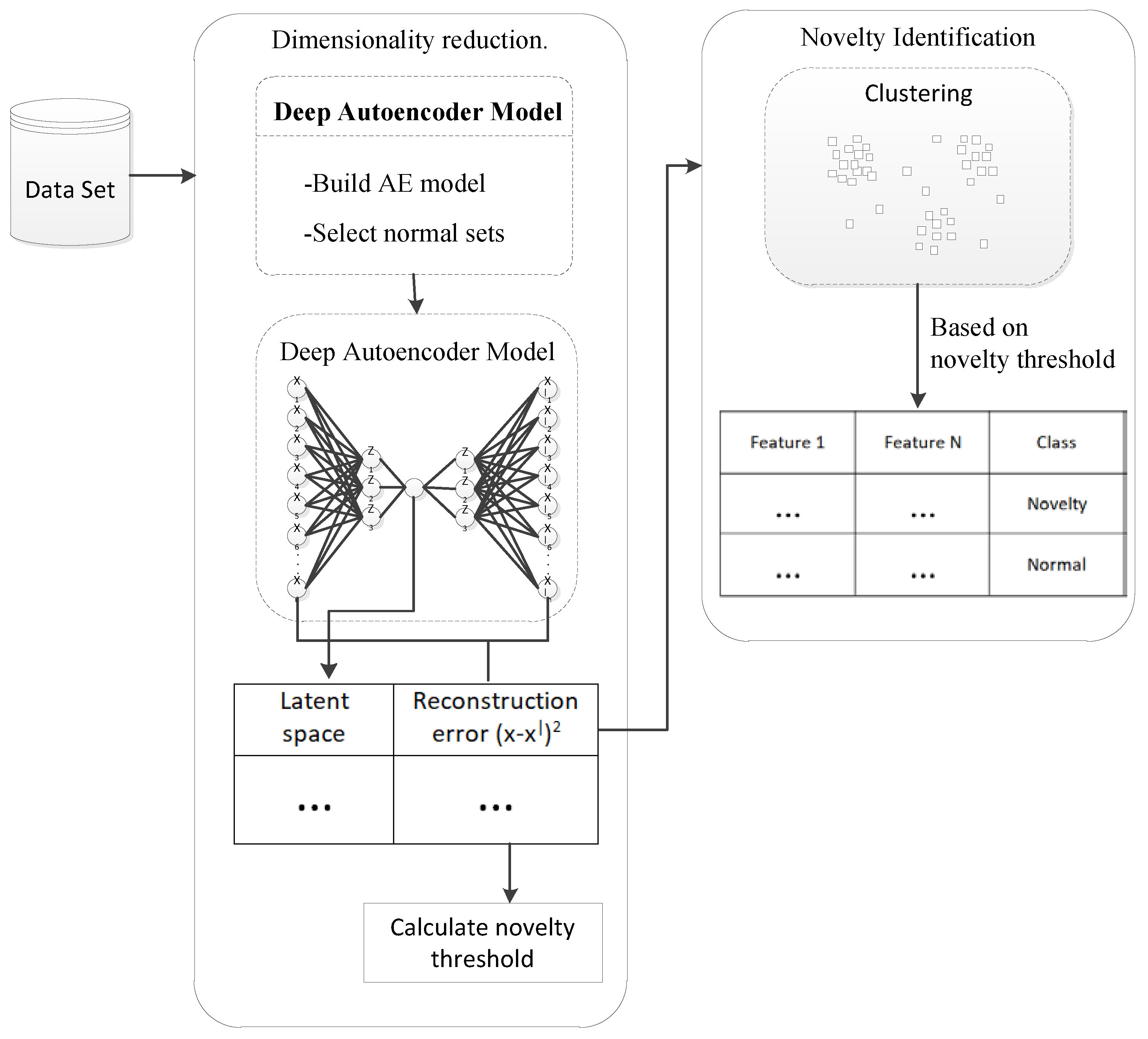
3. Methodology
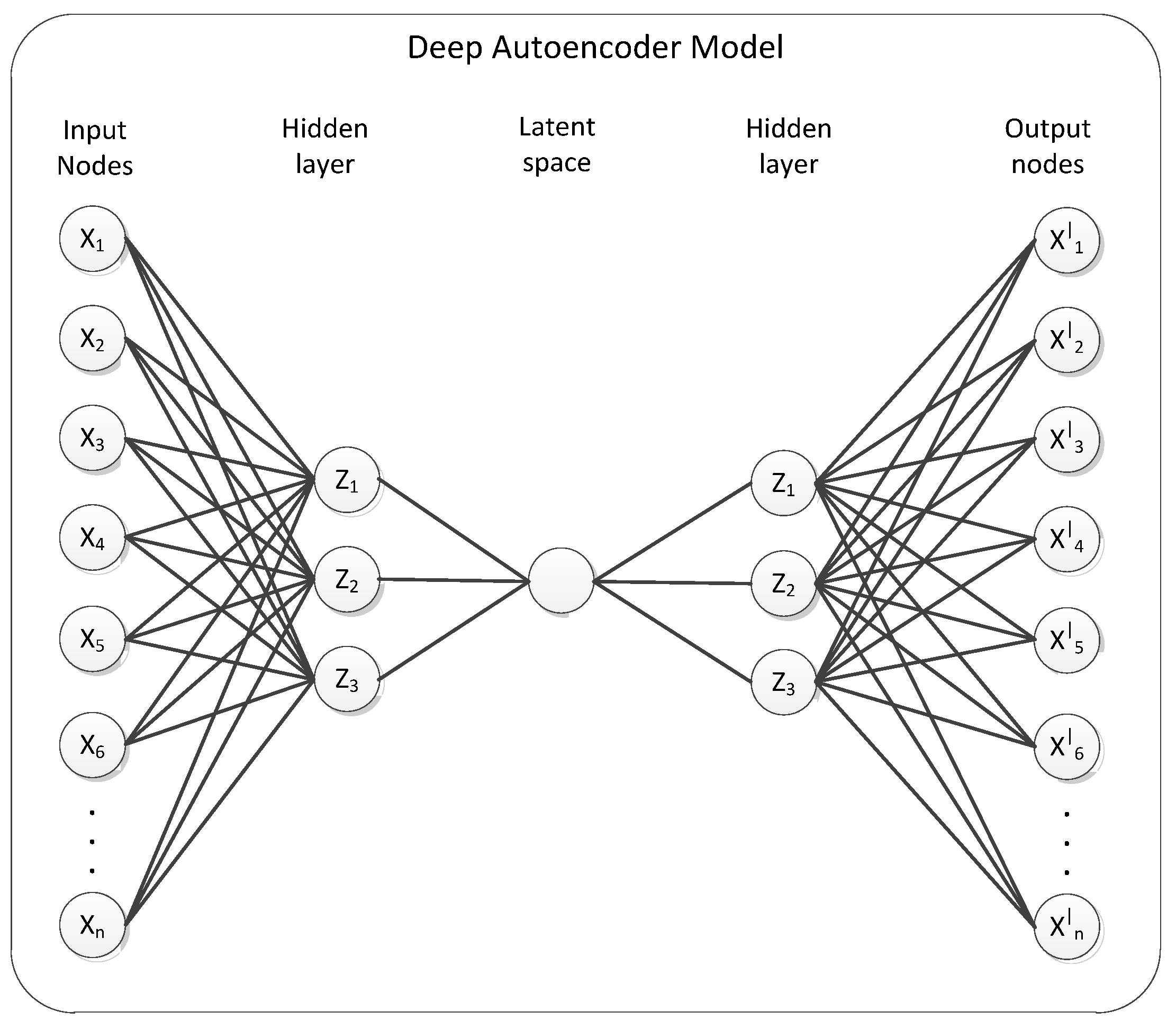
3.1. Deep Autoencoders for Dimensionality Reduction
| Algorithm 1: Dimensionality reduction. |
| 1: Input: Set of points 2: Output: Z |
| 3: inputLayer ← ( n_ nodes = n) 4: encoderLayer1 ← Dense(n_ nodes = n/2, activation = sigmoid)(inputLayer) 5: encoderLayer2 ← Dense(n_ nodes = 1, activation = sigmoid)(encoderLayer1) 6: decoderLayer1 ← Dense(n_ nodes = n/2, activation = tanh)(encoderLayer2) 7: decoder _layer2 ← Dense(n_ nodes = n, activation = tanh)(decoderLayer1) 8: AEModel ← Model(input_layer, decoder _layer2) 9: AEModel.fit(X) 10: ← AEModel.predict(X) |
| 11: reconstructionError ← [] 12: for i=0 to do 13: reconstructionErrori ← 2 14: end for |
| 15: threshold ← Otsu(reconstructionError) 16: X[reconstructionError] ← reconstructionError |
| 17: norms ← (X [reconstructionrError] < threshold) |
| 18: AEModel.fit(norms) 19: ← AEModel.predict(X) 20: E ← AEModel. encoderLayer2 |
| 21: reconstructionError ← [] 22: for i to do 23: reconstructionErrori ← 2 24: end for |
| 25: finalThreshold ← Otsu(reconstructionError) |
| 26: Z ← [] 27: Z[encoded] ← E 28: Z[error] ← reconstructionError 29: return Z |
- Run-time complexity of backpropagation of autoencoder model is O(epochs*training example*(number of weights))
- Prediction process is O(n)
- Calculate reconstruction errors from decoded output and input is O(n)
- Calculate novelty threshold is O(n)
3.2. Density Based Clustering for Novelty Detection
- Calculate nearest neighbors is O(dn3) where d is dimension and n is the number of samples
- DBSCAN clustering is O(n2)
- Identify novelty is O(n)
| Algorithm 2: Identify novelty. |
| 1: Input: Set of points , set op points X, 2: Output: X, #with decision |
| 3: nbrs ← NearestNeighbors (n_neighbors=3).fit (Z) 4: distance ← nbrs.kneighbors (Z) 5: distance.sort() 6: eps ← first extreme value of distance |
| 7: cluster ← dbscan(Z, eps) 8: n_clusters ← len(cluster.labels_) 9: X[labels] ← cluster.labels_ |
| 10: dict_error ← {} 11: for i=0 to n_clusters do 12: bool_values ← (X [labels_] == i ) 13: cluster_i_set ← Z[boolvalues] 14: n_instance_in_cluster_i = len(cluster_i_set) 15: error_count = 0 16: for j in n_instance_in_cluster_i do 17: if cluster_i_set[j] > final_threshold 18: error_count ← error_count + 1 19: endif 20: end for 21: dict_error[i] ← error_count 22: end for 23: for i=0 to n_clusters do 24: cluster_i ← X[db_labels == i] 25: n_of_instance ← len(cluster_i) 26: if n_of_instance * 0.5 less than or equal to dict_error.get(i) 27: X.update[ all rows in cluster, labels ] = 1 #novelty 28: else 29: X. update[ all rows in cluster, labels ] = 0 #normal 30: endif 31: end for 32: return X |
| Algorithm 3: DAE-DBC algorithm. |
| 1: Input: Set of points 2: Output: Y, { #decision |
| 3: Z ← Dimensionality reduction(X) 4: Y ← Identify novelty(Z) 5: return Y |
4. Experimental Study
4.1. Datasets
4.2. Methods Compared
- OC-SVM. OC-SVM is used for novelty detection based on building prediction model from only normal dataset [23]. Eta-SVM and Robust SVM that an enhanced OC-SVM are introduced by Mennatallah et al. [20] and they suggest an implementation which is an extension of Rapidminer. We use this extension configured by RBF kernel function for these three algorithms.
- PCA based methods. PCA is commonly used for outlier detection and calculates the outlier score using the principal component scores and reconstruction error which is the orthogonal distance of each data point and its first principal component score. The Gaussian Mixture Model and Cumulative Distribution Function are used to make novelty detection decision from Outlier score [35,36]. We compare the PCA-based methods including PCA-GMM, PCA-CDF, Kernel PCA-GMM, Kernel PCA-CDF and Robust PCA [25].
- DAE-DBC (Proposed method). The structure of the deep autoencoder is composed of the 5 number of layers like {input layer (n neurons) → encoding layer (n/2 neurons) → encoding layer (1 neuron) → decoding layer (n/2 neurons) → decoding layer (n neuron)}, where n is the number of neurons. In here, the number of neurons in a bottleneck hidden layer which is the compressed representation of the original input is equal to one, other hidden layers are composed of neurons of about a half of the input neurons. The sigmoid activation function is used for encoding type-layers, the tanh activation function is for decoding-type layers respectively. Reconstruction error and compressed representation are grouped by density-based DBSCAN clustering algorithm and the novelty threshold will decide whether the group is the novelty.
- DAE-Kmeans. Compare with the proposed method using the K-means clustering algorithm instead of density-based clustering. K-means clustering algorithms require the number of cluster k and we have used Silhouettes analysis which is used for evaluation of clustering validity to find optimal k [37].
- PCA-DBC, KPCA-DBC. Our proposed method is based on reconstruction error. So, we have used PCA and KPCA in place of AE for calculating reconstruction error and compressed representation.
4.3. Evaluation Metrics
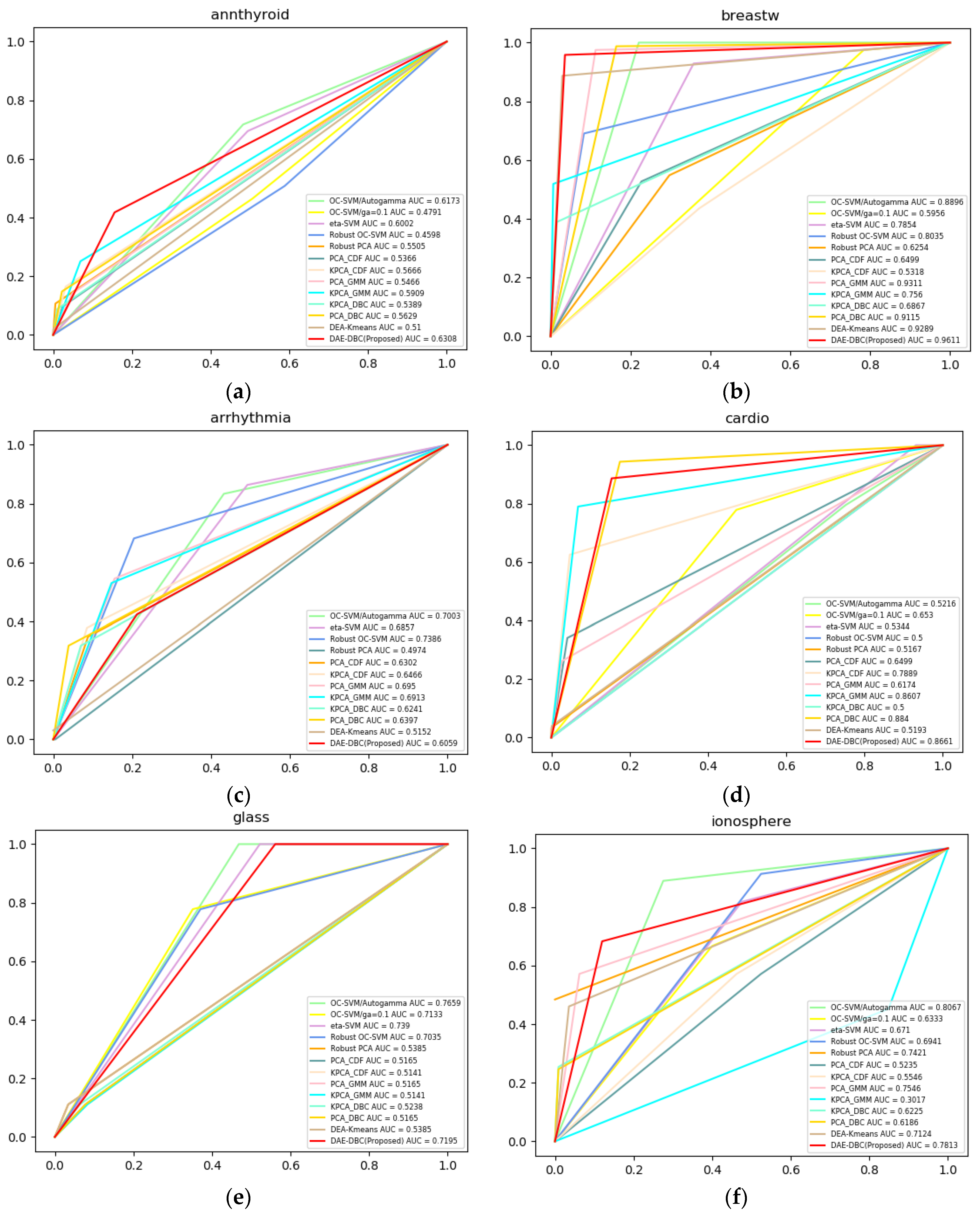
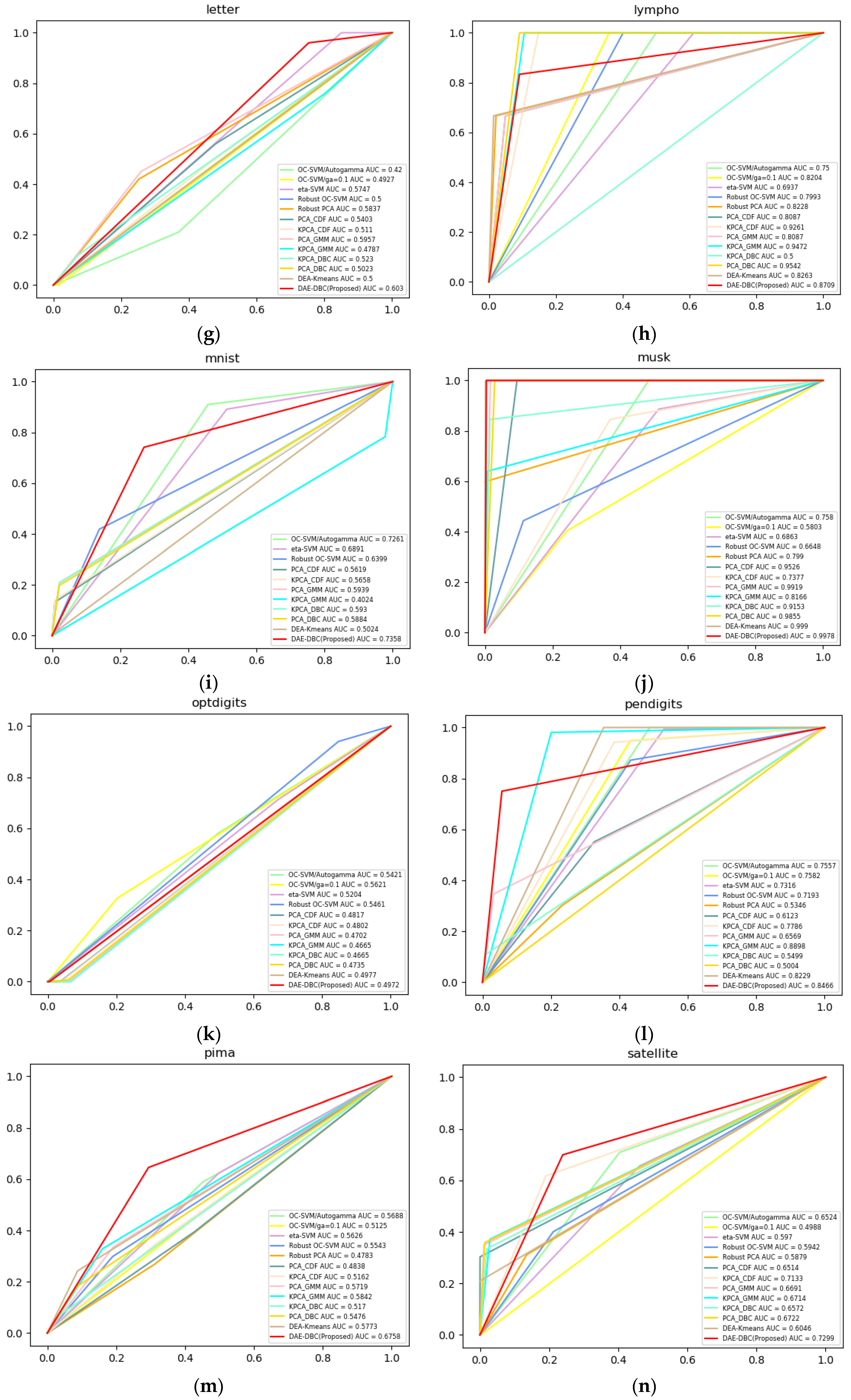
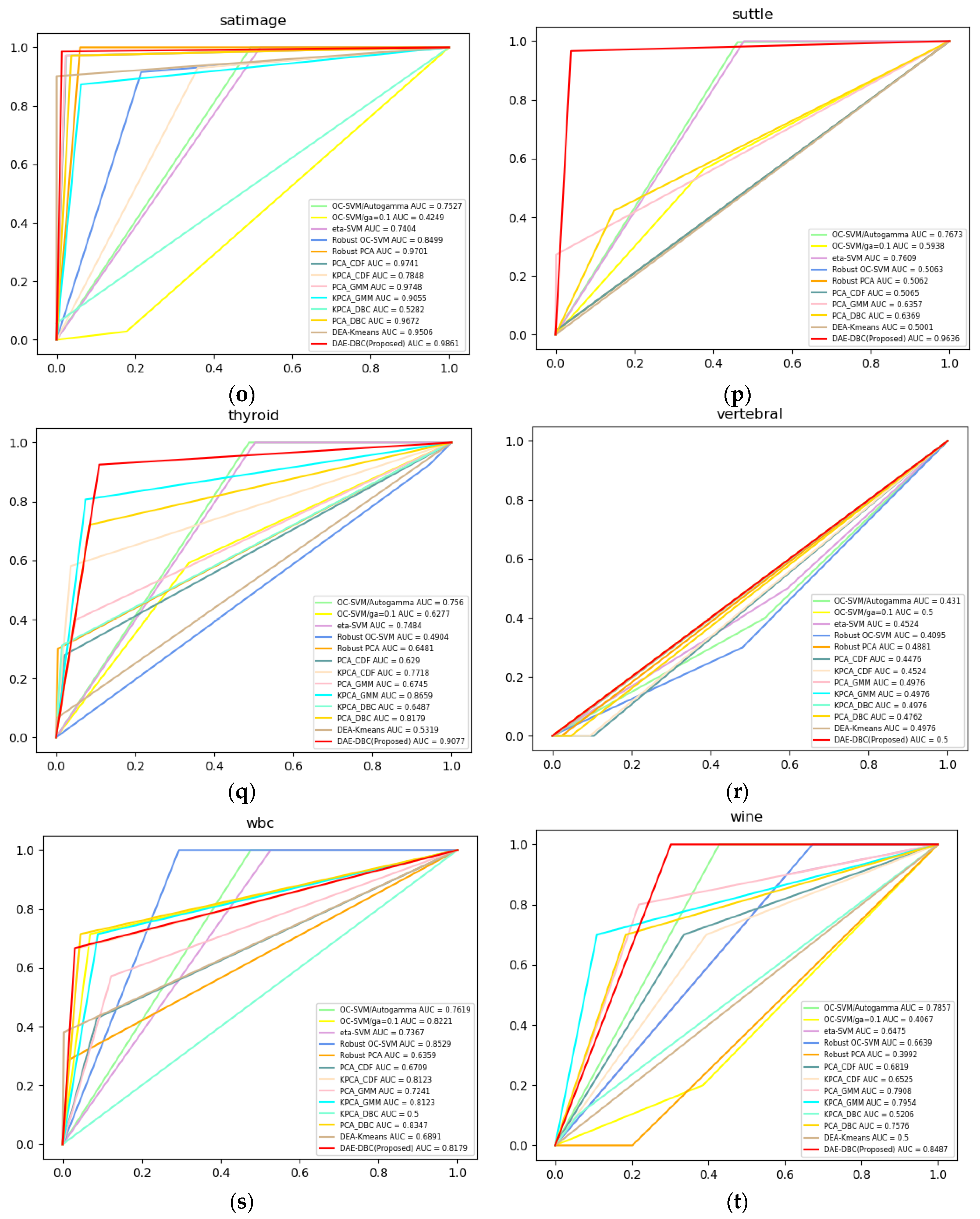
4.4. Experimental Result
5. Conclusions
Author Contributions
Funding
Conflicts of Interest
References
- Chandola, V.; Banerjee, A.; Kumar, V. Anomaly Detection: A Survey. ACM Comput. Surv. 2009, 41, 1–58. [Google Scholar] [CrossRef]
- Tan, P.N.; Steinbach, M.; Kumar, V. Anomaly Detection. In Introduction to Data Mining; Goldstein, M., Harutunian, K., Smith, K., Eds.; Pearson Education Inc.: Boston, MA, USA, 2006; pp. 651–680. ISBN 0-321-32136-7. [Google Scholar]
- Chalapathy, R.; Menon, A.K.; Chawla, S. Anomaly Detection using One-Class Neural Networks. arXiv, 2018; arXiv:1802.06360. [Google Scholar]
- Pascoal, C.; Oliveira, M.R.; Valadas, R.; Filzmoser, P.; Salvador, P.; Pacheco, A. Robust Feature Selection and Robust PCA for Internet Traffic Anomaly Detection. In Proceedings of the IEEE INFOCOM, Orlando, FL, USA, 25–30 March 2012. [Google Scholar]
- Kim, D.P.; Yi, G.M.; Lee, D.G.; Ryu, K.H. Time-Variant Outlier Detection Method on Geosensor Networks. In Proceedings of the International Symposium on Remote Sensing, Daejeon, Korea, 29–31 October 2008. [Google Scholar]
- Lyon, A.; Minchole, A.; Martınez, J.P.; Laguna, P.; Rodriguez, B. Computational techniques for ECG analysis and interpretation in light of their contribution to medical advances. J. R. Soc. Interface 2018, 15. [Google Scholar] [CrossRef] [PubMed]
- Anandakrishnan, A.; Kumar, S.; Statnikov, A.; Faruquie, T.; Xu, D. Anomaly Detection in Finance: Editors’ Introduction. In Proceedings of the Machine Learning Research, Halifax, Nova Scotia, 14 August 2017. [Google Scholar]
- Jin, C.H.; Park, H.W.; Wang, L.; Pok, G.; Ryu, K.H. Short-term Traffic Flow Forecasting using Unsupervised and Supervised Learning Techniques. In Proceedings of the 6th International Conference FITAT and 3rd International Symposium ISPM, Cheongju, Korea, 25–27 September 2013. [Google Scholar]
- Hauskrecht, M.; Batal, I.; Valko, M.; Visweswaran, S.; Cooper, C.F.; Clermont, G. Outlier detection for patient monitoring and alerting. J. Biomed. Inform. 2013, 46, 47–55. [Google Scholar] [CrossRef] [PubMed]
- Cho, Y.S.; Moon, S.C.; Ryu, K.S.; Ryu, K.H. A Study on Clinical and Healthcare Recommending Service based on Cardiovascula Disease Pattern Analysis. Int. J. Biosci. Biotechnol. 2016, 8, 287–294. [Google Scholar] [CrossRef]
- Chawla, N.V.; Japkowicz, N.; Kotcz, A. Editorial: Special Issue on Learning from Imbalanced Data Sets. SIGKDD Explor. Newsl. 2004, 6, 1–6. [Google Scholar] [CrossRef]
- Sarah, M.E.; Rajasegarar, S.; Karunasekera, S.; Leckie, C. High-dimensional and large-scale anomaly detection using a linear one-class SVM with deep learning. Pattern Recognit. 2016, 58, 121–134. [Google Scholar]
- Zimek, A.; Schubert, E.; Kriegel, H.P. A survey on unsupervised outlier detection in high-dimensional numerical data. Stat. Anal. Data Min. 2012, 5, 363–387. [Google Scholar] [CrossRef]
- Rousseeuw, P.J.; Hubert, M. Anomaly Detection by Robust Statistics. WIREs Data Min. Knowl Discov. 2018, 8, 1–30. [Google Scholar] [CrossRef]
- Hoffmann, H. Kernel PCA for novelty detection. Pattern Recognit. 2007, 40, 863–874. [Google Scholar] [CrossRef]
- Zong, B.; Song, Q.; Min, M.R.; Cheng, W.; Lumezanu, C.; Cho, D.; Chen, H. Deep autoencoding gaussian mixture model for unsupervised anomaly detection. In Proceedings of the 6th International Conference on Learning Representations, Vancouver, BC, Canada, 30 April–3 May 2018. [Google Scholar]
- Protopapadakis, E.; Voulodimos, A.; Doulamis, A.; Doulamis, N.; Dres, D.; Bimpas, M. Stacked Autoencoders for Outlier Detection in Over-the-Horizon Radar Signals. Comput. Intell. Neurosci. 2017, 2017. [Google Scholar] [CrossRef] [PubMed]
- Kim, H.; Hirose, A. Unsupervised Fine Land Classification Using Quaternion Autoencoder-Based Polarization Feature Extraction and Self-Organizing Mapping. IEEE Trans. Geosci. Remote Sens. 2018, 56, 1839–1851. [Google Scholar] [CrossRef]
- Elbatta, M.T.; Ashour, W.M. A Dynamic Method for Discovering Density Varied Clusters. International Journal of Signal Processing. Image Process. Pattern Recognit. 2013, 6, 123–134. [Google Scholar]
- Amer, M.; Goldstein, M.; Abdennadher, S. Enhancing One-class Support Vector Machines for Unsupervised Anomaly Detection. In Proceedings of the ACM SIGKDD Workshop on Outlier Detection and Description, Chicago, IL, USA, 11 August 2013. [Google Scholar]
- Ghafoori, Z.; Erfani, S.M.; Rajasegarar, S.; Bezdek, J.C.; Karunasekera, S.; Leckie, C. Efficient Unsupervised Parameter Estimation for One-Class Support Vector Machines. IEEE Trans. Neural Netw. Learn. Syst. 2018, 1–14. [Google Scholar] [CrossRef] [PubMed]
- Yin, S.; Zhu, X.; Jing, C. Fault Detection Based on a Robust One Class Support Vector Machine. Neurocomputing 2014, 145, 263–268. [Google Scholar] [CrossRef]
- Schölkopf, B.; Williamson, R.; Smola, A.; Shawe-Taylor, J.; Platt, J. Support Vector Method for Novelty Detection. In Proceedings of the 12th International Conference on Neural Information Processing Systems, Cambridge, MA, USA, 29 November–4 December 1999. [Google Scholar]
- Zaki, M.J.; Wagner, M., Jr. Data Mining and Analysis: Fundamental Concepts and Algorithms; Cambridge University Press: New York, NY, USA, 2014; ISBN 978-0-521-76633-3. [Google Scholar]
- Kwitt, R.; Hofmann, U. Robust Methods for Unsupervised PCA-based Anomaly Detection. In Proceedings of the IEEE/IST Workshop on “Monitoring, Attack Detection and Mitigation”, Tuebingen, Germany, 28–29 September 2006. [Google Scholar]
- Zhang, Y.D.; Zhang, Y.; Hou, X.X.; Chen, H.; Wang, S.H. Seven-Layer Deep Neural Network Based on Sparse Autoencoder for Voxelwise Detection of Cerebral Microbleed. Multimedia Tools Appl. 2018, 77, 10521–10538. [Google Scholar] [CrossRef]
- Jia, W.; Muhammad, K.; Wang, S.H.; Zhang, Y.D. Five-Category Classification of Pathological Brain Images Based on Deep Stacked Sparse Autoencoder. Multimedia Tools Appl. 2017, 77, 1–20. [Google Scholar] [CrossRef]
- Liou, C.; Cheng, W.; Liou, J.; Liou, D. Autoencoder for Words. Neurocomputing 2014, 139, 84–96. [Google Scholar] [CrossRef]
- Guo, Y.; Liu, Y.; Oerlemans, A.; Lao, S.; Wu, S.; Lew, M.S. Deep Learning for Visual Understanding: A review. Neurocomputing 2016, 187, 27–48. [Google Scholar] [CrossRef]
- Otsu, N. A Threshold Selection Method from Gray-Level Histograms. IEEE Trans. Syst. Man Cybern. 1979, 9, 62–66. [Google Scholar] [CrossRef]
- Ester, M.; Kriegel, H.P.; Sander, J.; Xu, X. A Density-Based Algorithm for Discovering Clusters in Large Spatial Databases with Noise. KDD-96 Proc. 1996, 96, 226–231. [Google Scholar]
- Hodge, V.; Austin, J. A Survey of Outlier Detection Methodologies. Artif. Intell. Rev. 2004, 22, 85–126. [Google Scholar] [CrossRef]
- Bellman, R.E. Adaptive Control Processes: A Guided Tour; Princeton University Press: Princeton, NJ, USA, 1961; ISBN 9781400874668. [Google Scholar]
- Rayana, S. ODDS. Stony Brook University, Department of Computer Sciences, 2016. Available online: http://odds.cs.stonybrook.edu/ (accessed on 30 July 2018).
- Yu, J. Fault Detection Using Principal Components-Based Gaussian Mixture Model for Semiconductor Manufacturing Processes. IEEE Trans. Semicond. Manuf. 2011, 24, 432–444. [Google Scholar] [CrossRef]
- Kim, J.; Grauman, K. Observe locally, infer globally: A space-time MRF for detecting abnormal activities with incremental updates. In Proceedings of the IEEE Conference on Computer Vision and Pattern Recognition, Miami, FL, USA, 20–25 June 2009. [Google Scholar]
- Rousseeuw, P.J. Silhouettes: A Graphical Aid to the Interpretation and Validation of Cluster Analysis. J. Comput. Appl. Math. 1987, 20, 53–65. [Google Scholar] [CrossRef]
- Kingma, D.P.; Ba, J. Adam: A method for stochastic optimization. In Proceedings of the 3rd International Conference for Learning Representations, San Diego, CA, USA, 7–9 May 2014. [Google Scholar]


| Dataset | Dim | Instance | Normal | Novelty | Description |
|---|---|---|---|---|---|
| BreastW | 10 | 683 | 444 | 239 | There are two classes, benign and malignant. The malignant class is considered as novelty. |
| Annthyroid | 6 | 7200 | 6666 | 534 | There are three classes are built: normal, hyperfunction and subnormal functioning. The hyperfunction and subnormal classes are treated as novelty class. |
| Arrhythmia | 274 | 452 | 386 | 66 | It is a multi-class classification dataset. The smallest classes, i.e., 3, 4, 5, 7, 8, 9, 14, 15 are combined to form the novelty class. |
| Cardio | 21 | 1831 | 1655 | 176 | There are 3 classes, normal, suspect and pathologic. Pathologic (novelty) class is downsampled to 176 points. The suspect class is discarded. |
| Glass | 9 | 214 | 205 | 9 | This dataset contains attributes regarding several glass types (multi-class). Here, class 6 is marked as novelty. |
| Ionosphere | 33 | 351 | 225 | 126 | There is one attribute having values all zeros, which is discarded. So, the total number of dimensions are 33. The ‘bad’ class is considered as novelty class. |
| Letter | 32 | 1600 | 1500 | 100 | 3 letters from data was sampled to form the normal class and randomly concatenate pairs of them to form the novelty class. |
| Lympho | 18 | 148 | 142 | 6 | It has four classes but two of them are quite small. Therefore, those two small classes are merged and considered as novelty. |
| Mnist | 100 | 7603 | 6903 | 700 | Digit-zero class is considered as inliers, while 700 images are sampled from digit-six class as the outliers. |
| Musk | 72 | 3062 | 2965 | 97 | The non-musk classes, j146, j147 and 252 are combined to form the inliers, while the musk classes 213 and 211 are added as novelty without downsampling. Other classes are discarded. |
| Optdigits | 64 | 5216 | 5066 | 150 | The instances of digits 1-9 are inliers and instances of digit 0 are down-sampled to 150 outliers. |
| Pendigits | 16 | 6870 | 6714 | 156 | It has10 classes (0 … 9). In this dataset, all classes have equal frequencies. So, the number of objects in one class (corresponding to the digit “0”) is reduced by a factor of 10%. |
| Pima | 8 | 768 | 500 | 268 | Several constraints were placed on the selection of instances from a larger database. In particular, all patients here are females at least 21 years old of Pima Indian heritage. |
| Satellite | 36 | 6435 | 4399 | 2036 | The smallest three classes, i.e., 2, 4, 5 are combined to form the outliers’ novelty. |
| Satimage | 36 | 5803 | 5732 | 71 | Class 2 is down-sampled to 71 outliers, while all the other classes are combined to form an inlier class. |
| Suttle | 9 | 49097 | 45586 | 3511 | The smallest 5 classes, i.e., 2, 3, 5, 6, 7 are combined to form the novelty class, while class 1 forms the inlier class. Data for class 4 is discarded. |
| Thyroid | 6 | 3772 | 3679 | 93 | There are 3 classes are built: normal, hyperfunction and subnormal functioning. The hyperfunction class is treated as novelty class. |
| Vertebral | 6 | 240 | 210 | 30 | The following convention is used for the class labels: Normal (NO) and Abnormal (AB). Here, “AB” is the majority class having 210 instances which are used as inliers and “NO” is downsampled from 100 to 30 instances as outliers. |
| WBC | 30 | 378 | 357 | 21 | There are 2 classes, benign and malignant. The malignant class of this dataset is downsampled to 21 points, which are considered as novelty. |
| Wine | 13 | 129 | 119 | 10 | Class 1 is downsampled to 10 instances to be used as novelty. |
| Dataset | Algorithm 1 | Algorithm 3 |
|---|---|---|
| Annthyroid | 0.5866 | 0.6308 |
| Breastw | 0.8962 | 0.9767 |
| Arrhythmia | 0.9181 | 0.6966 |
| Cardio | 0.7837 | 0.8661 |
| Glass | 0.4580 | 0.7195 |
| Ionosphere | 0.7440 | 0.7813 |
| Letter | 0.5957 | 0.6030 |
| Lympho | 0.7500 | 0.8709 |
| Mnist | 0.7315 | 0.7358 |
| Musk | 0.9266 | 0.9978 |
| Optdigits | 0.6108 | 0.4972 |
| Pendigits | 0.7861 | 0.8466 |
| Pima | 0.6423 | 0.6758 |
| Satellite | 0.6696 | 0.7299 |
| Satimage | 0.9204 | 0.9861 |
| Suttle | 0.9427 | 0.9695 |
| Thyroid | 0.9554 | 0.9077 |
| Vertebral | 0.4000 | 0.5000 |
| Wbc | 0.8221 | 0.8179 |
| Wine | 0.8487 | 0.8487 |
| RapidMiner/Extension of Outlier Detection/ | Python Implementation/Using Keras/ | ||||||||||||
|---|---|---|---|---|---|---|---|---|---|---|---|---|---|
| Dataset | OC-SVM /auto gamma, nu=0.5/ | OC-SVM /gamma=0.1, nu=0.5/ | eta-SVM /auto gamma, nu=0.5/ | Robust-SVM /auto gamma, nu=0.5/ | Robust-PCA | PCA-CDF | KPCA-CDF | PCA-GMM | KPCA-GMM | PCA-DBC | KPCA-DBC | DAE-Kmeans | DAE-DBC (Proposed) |
| Annthyroid | 0.6173 | 0.4791 | 0.6002 | 0.4598 | 0.5505 | 0.5366 | 0.5666 | 0.5466 | 0.5909 | 0.5629 | 0.5389 | 0.5100 | 0.6308 |
| Breastw | 0.8896 | 0.5956 | 0.7854 | 0.8035 | 0.6254 | 0.6499 | 0.5318 | 0.9311 | 0.7560 | 0.9115 | 0.6867 | 0.9289 | 0.9767 |
| Arrhythmia | 0.7003 | NA | 0.6857 | 0.7386 | 0.4974 | 0.6302 | 0.6466 | 0.6950 | 0.6913 | 0.6397 | 0.6241 | 0.5152 | 0.6966 |
| Cardio | 0.5216 | 0.6530 | 0.5344 | 0.5000 | 0.5167 | 0.6499 | 0.7889 | 0.6174 | 0.8607 | 0.8840 | 0.5000 | 0.5193 | 0.8661 |
| Glass | 0.7659 | 0.7133 | 0.7390 | 0.7035 | 0.5385 | 0.5165 | 0.5141 | 0.5165 | 0.5141 | 0.5165 | 0.5238 | 0.5385 | 0.7195 |
| Ionosphere | 0.8067 | 0.6333 | 0.6710 | 0.6941 | 0.7421 | 0.5235 | 0.5546 | 0.7546 | 0.3017 | 0.6186 | 0.6225 | 0.7124 | 0.7813 |
| Letter | 0.4200 | 0.4927 | 0.5747 | 0.5000 | 0.5837 | 0.5403 | 0.7400 | 0.5957 | 0.4787 | 0.5023 | 0.5230 | 0.5000 | 0.6030 |
| Lympho | 0.7500 | 0.8204 | 0.6937 | 0.7993 | 0.8228 | 0.8087 | 0.9261 | 0.8087 | 0.9472 | 0.9542 | 0.5000 | 0.8263 | 0.8709 |
| Mnist | 0.7261 | NA | 0.6891 | 0.6399 | NA | 0.5619 | 0.5658 | 0.5939 | 0.4024 | 0.5884 | 0.5930 | 0.5024 | 0.7358 |
| Musk | 0.7580 | 0.5803 | 0.6863 | 0.6648 | 0.7990 | 0.9526 | 0.7377 | 0.9919 | 0.8166 | 0.9855 | 0.9153 | 0.9990 | 0.9978 |
| Optdigits | 0.5421 | 0.5621 | 0.5204 | 0.5461 | NA | 0.4817 | 0.4980 | 0.4702 | 0.4665 | 0.4735 | 0.4665 | 0.8229 | 0.4972 |
| Pendigits | 0.7557 | 0.7582 | 0.7316 | 0.7193 | 0.5346 | 0.6123 | 0.7786 | 0.6569 | 0.8898 | 0.5004 | 0.5499 | 0.6926 | 0.8466 |
| Pima | 0.5688 | 0.5125 | 0.5626 | 0.5543 | 0.4783 | 0.4838 | 0.5162 | 0.5719 | 0.5842 | 0.5476 | 0.5170 | 0.5773 | 0.6758 |
| Satellite | 0.6524 | 0.4988 | 0.5970 | 0.5942 | 0.5879 | 0.6514 | 0.7133 | 0.6691 | 0.6714 | 0.6722 | 0.6572 | 0.6046 | 0.7299 |
| Satimage | 0.7527 | 0.4249 | 0.7404 | 0.8499 | 0.9701 | 0.9741 | 0.7848 | 0.9748 | 0.9055 | 0.9672 | 0.5282 | 0.9506 | 0.9861 |
| Suttle | 0.7673 | 0.5938 | 0.7609 | 0.5063 | 0.5062 | 0.5065 | NA | 0.6357 | NA | 0.6369 | NA | 0.5001 | 0.9695 |
| Thyroid | 0.7560 | 0.6277 | 0.7484 | 0.4904 | 0.6481 | 0.6290 | 0.7718 | 0.6745 | 0.8659 | 0.8179 | 0.6487 | 0.5319 | 0.9077 |
| Vertebral | 0.4310 | 0.5000 | 0.4524 | 0.4095 | 0.4881 | 0.4476 | 0.4524 | 0.4976 | 0.4976 | 0.4762 | 0.4976 | 0.4976 | 0.5000 |
| Wbc | 0.7619 | 0.8221 | 0.7367 | 0.8529 | 0.6359 | 0.6709 | 0.8123 | 0.7241 | 0.8123 | 0.8347 | 0.5000 | 0.6891 | 0.8179 |
| Wine | 0.7857 | 0.4067 | 0.6475 | 0.6639 | 0.3992 | 0.6819 | 0.6525 | 0.7908 | 0.7954 | 0.7576 | 0.5206 | 0.5000 | 0.8487 |
| Average AUC | 0.6865 | 0.5930 | 0.6579 | 0.6345 | 0.6069 | 0.6255 | 0.6606 | 0.6858 | 0.6762 | 0.6924 | 0.5744 | 0.6459 | 0.7829 |
| RapidMiner/Extension of Outlier Detection/ | Python Implementation/Using Keras/ | ||||||||||||
|---|---|---|---|---|---|---|---|---|---|---|---|---|---|
| Dataset | OC-SVM /auto gamma, nu=0.5/ | OC-SVM /gamma=0.1, nu=0.5/ | eta-SVM /auto gamma, nu=0.5/ | Robust-SVM /auto gamma, nu=0.5/ | Robust-PCA | PCA-CDF | KPCA-CDF | PCA-GMM | KPCA-GMM | PCA-DBC | KPCA-DBC | DAE-Kmeans | DAE-DBC (Proposed) |
| Annthyroid | 40 | 66 | 46 | 46 | 0.11 | 0.25 | 24.662 | 0.467 | 28.491 | 26.576 | 33.581 | 2002.1 | 261.46 |
| Breastw | 44 | 7 | 46 | 6 | 0.153 | 0.463 | 0.477 | 0.492 | 0.666 | 22.22 | 21.874 | 115.32 | 31.764 |
| Arrhythmia | 0< | NA | 1 | 0< | 0.063 | 0.082 | 0.206 | 0.111 | 0.394 | 6.737 | 9.155 | 105.33 | 32.916 |
| Cardio | 12 | 24 | 15 | 16 | 0.107 | 0.227 | 1.564 | 0.326 | 1.824 | 9.027 | 7.735 | 152.27 | 71.649 |
| Glass | 0< | 0< | 0< | 0< | 0.025 | 0.034 | 0.059 | 0.084 | 0.156 | 8.164 | 5.286 | 32.869 | 14.515 |
| Ionosphere | 0< | 0< | 0< | 0< | 0.041 | 0.069 | 0.115 | 0.138 | 0.263 | 32.845 | 5.919 | 39.85 | 19.17 |
| Letter | 5 | 11 | 7 | 7 | 0.072 | 0.267 | 1.349 | 0.315 | 1.574 | 9.577 | 9.775 | 113.1 | 60.347 |
| Lympho | 0< | 0< | 0< | 0< | 0.027 | 0.041 | 0.164 | 0.077 | 0.219 | 3.613 | 7.435 | 22.957 | 15.056 |
| Mnist | 1330 | NA | 1134 | 1111 | NA | 3.378 | 41.538 | 2.789 | 43.302 | 27.391 | 35.814 | 754.57 | 268.66 |
| Musk | 50 | 90 | 71 | 73 | 0.204 | 0.691 | 6.714 | 0.660 | 7.116 | 10.253 | 10.989 | 322.09 | 136.11 |
| Optdigits | 124 | 201 | 142 | 146 | NA | 0.923 | 15.405 | 0.997 | 16.585 | 29.792 | 21.358 | 509.33 | 180.97 |
| Pendigits | 31 | 42 | 31 | 36 | 0.262 | 0.561 | 23.313 | 0.656 | 24.260 | 23.485 | 30.98 | 637.16 | 221.27 |
| Pima | 0< | 0< | 0< | 0< | 0.037 | 0.112 | 0.360 | 0.166 | 0.497 | 7.867 | 5.266 | 80.555 | 28.045 |
| Satellite | 66 | 96 | 71 | 78 | 0.207 | 0.685 | 21.680 | 0.798 | 24.556 | 22.789 | 58.857 | 686.85 | 236.33 |
| Satimage | 42 | 58 | 44 | 55 | 0.187 | 0.642 | 17.275 | 0.849 | 18.386 | 2.419 | 21.31 | 592.40 | 217.29 |
| Suttle | 19,908 | 19,761 | 22,431 | 22,891 | 0.577 | 1.437 | NA | 1.780 | NA | 139.98 | NA | 5419.4 | 1753.7 |
| Thyroid | 13 | 18 | 15 | 17 | 0.088 | 0.207 | 5.677 | 0.271 | 6.097 | 13.092 | 17.961 | 328.83 | 218.54 |
| Vertebral | 0< | 0< | 0< | 0< | 0.07 | 0.060 | 0.060 | 0.107 | 0.111 | 4.497 | 9.151 | 37.441 | 20.874 |
| Wbc | 0< | 0< | 0< | 0< | 0.05 | 0.148 | 0.166 | 0.169 | 0.212 | 4.043 | 3.269 | 72.288 | 46.738 |
| Wine | 0< | 0< | 0< | 0< | 0.028 | 0.055 | 0.044 | 0.083 | 0.098 | 3.929 | 8.441 | 20.71 | 26.951 |
© 2018 by the authors. Licensee MDPI, Basel, Switzerland. This article is an open access article distributed under the terms and conditions of the Creative Commons Attribution (CC BY) license (http://creativecommons.org/licenses/by/4.0/).
Share and Cite
Amarbayasgalan, T.; Jargalsaikhan, B.; Ryu, K.H. Unsupervised Novelty Detection Using Deep Autoencoders with Density Based Clustering. Appl. Sci. 2018, 8, 1468. https://doi.org/10.3390/app8091468
Amarbayasgalan T, Jargalsaikhan B, Ryu KH. Unsupervised Novelty Detection Using Deep Autoencoders with Density Based Clustering. Applied Sciences. 2018; 8(9):1468. https://doi.org/10.3390/app8091468
Chicago/Turabian StyleAmarbayasgalan, Tsatsral, Bilguun Jargalsaikhan, and Keun Ho Ryu. 2018. "Unsupervised Novelty Detection Using Deep Autoencoders with Density Based Clustering" Applied Sciences 8, no. 9: 1468. https://doi.org/10.3390/app8091468
APA StyleAmarbayasgalan, T., Jargalsaikhan, B., & Ryu, K. H. (2018). Unsupervised Novelty Detection Using Deep Autoencoders with Density Based Clustering. Applied Sciences, 8(9), 1468. https://doi.org/10.3390/app8091468