Article

Optimisation of the Structure of a Wind Farm—Kinetic Energy Storage for Improving the Reliability of Electricity Supplies

by
Andrzej Tomczewski
and
Leszek Kasprzyk
*
Faculty of Electrical Engineering, Poznań University of Technology, Piotrowo 3A str., 60-965 Poznań, Poland
*
Author to whom correspondence should be addressed.
Appl. Sci. 2018, 8(9), 1439; https://doi.org/10.3390/app8091439
Submission received: 15 July 2018 / Revised: 15 August 2018 / Accepted: 20 August 2018 / Published: 23 August 2018
(This article belongs to the Special Issue Large Grid-Connected Wind Turbines)

Abstract

:
An important issue in the correct operation of the power system is the reliability of the electricity supply from generation systems. This particular problem especially concerns renewable sources, the output power of which is variable over time and additionally has a stochastic character. The solution used in the work to improve the reliability indicators of wind farm sources is the partial stabilization of their output power achieved through cooperation with the kinetic energy storage. Excessive increase in storage capacity is associated with a large increase in investment and operating costs. It is therefore important to determine the minimum storage capacity required to maintain the accepted criteria for the reliability of energy supply. In this paper, a population meta-heuristics algorithm was used for this purpose. The obtained results confirm the possibility of limiting the energy capacity of the flywheels, they also indicate its non-linear character as a function of selected parameters of the reliability of energy supplies from wind farms.

1. Introduction

The prospect of exhausting fuel resources, air pollution, growing environmental awareness and legal regulations contribute to the increasing popularity of renewable energy sources for the production of electricity (RES-E). This trend can be observed for both low-power sources, which typically supply individual facilities (including, in particular, photovoltaic systems) and high-power facilities, such as water power plantsas well as wind and photovoltaic farms [1,2]. In some countries, the share of renewable energy sources (RES) in the power grid is greater than the share of conventional sources (Norway is the leader in this field; 98% of electricity in Norway is generated by renewable power plants—mainly water power plants) [3,4,5]. Few EU countries can boast such a high share of renewable sources in power generation. According to the “Renewable energy in Europe—2017 Update” report, on average, about 30% of electricity in member-states was generated from renewable sources [3].
One should pay attention to the fact that a dynamic increase in the number of renewable energy sources has some disadvantages related to a lack of power generation stability, which depends on the current weather conditions and low operating inertia. The problem applies especially to solar and wind sources. Heterogeneity can stabilise the operation of a power grid. It involves a high share of prosumer solutions and integration by means of intelligent systems (e.g., power generation predictions). Another solution is to use energy storage units, which can buffer the generated power (e.g., power generated by photovoltaic systems during the day will be released at night). Unfortunately, in the area of electrical power engineering, the existing energy storage systems are insufficient on a large scale, except for pumped-storage power stations (and thermal storages in southern countries). Moreover, it is expensive to build new energy storage systems (ESS) intended to work with RES-E. The cost can reach thousands of Euro/kWh in the case of electrical-chemical and kinetic storage units [6,7,8]. This is why scientific centres worldwide carry out research on ESS that can function in conjunction with RES-E, especially photovoltaic cells and wind turbines. References [9,10,11,12,13,14,15] focused on the issue of predicting the generating capacity of RES-E to adapt in advance with the power generated by other systems. There are the examples of papers [16,17,18,19,20,21,22,23,24] concern with the selection of the structure of energy sources and storages according to location needs and conditions. The assessment of the ESS effectiveness and profitability of their use is of paramount importance. The issue was mentioned in papers [2,12,22,23].
However, the literature, does not provide exhaustive information on the reliability of electrical energy generation in the context of the contribution of unstable renewable sources to the power grid. This is why the authors decided to concentrate on the topic of cooperation between wind farms and kinetic energy storage. Minimising the volume of ESS fulfils the set criterion including the reduction of costs related to the RES-E and ESS system installation. Analyses were carried out using historical wind speed data and, hence, the identified indicators are not probabilities or expected values but specific values identified for the specific analysis period.

2. Characteristics of a Wind Farm—Kinetic Energy Storage System

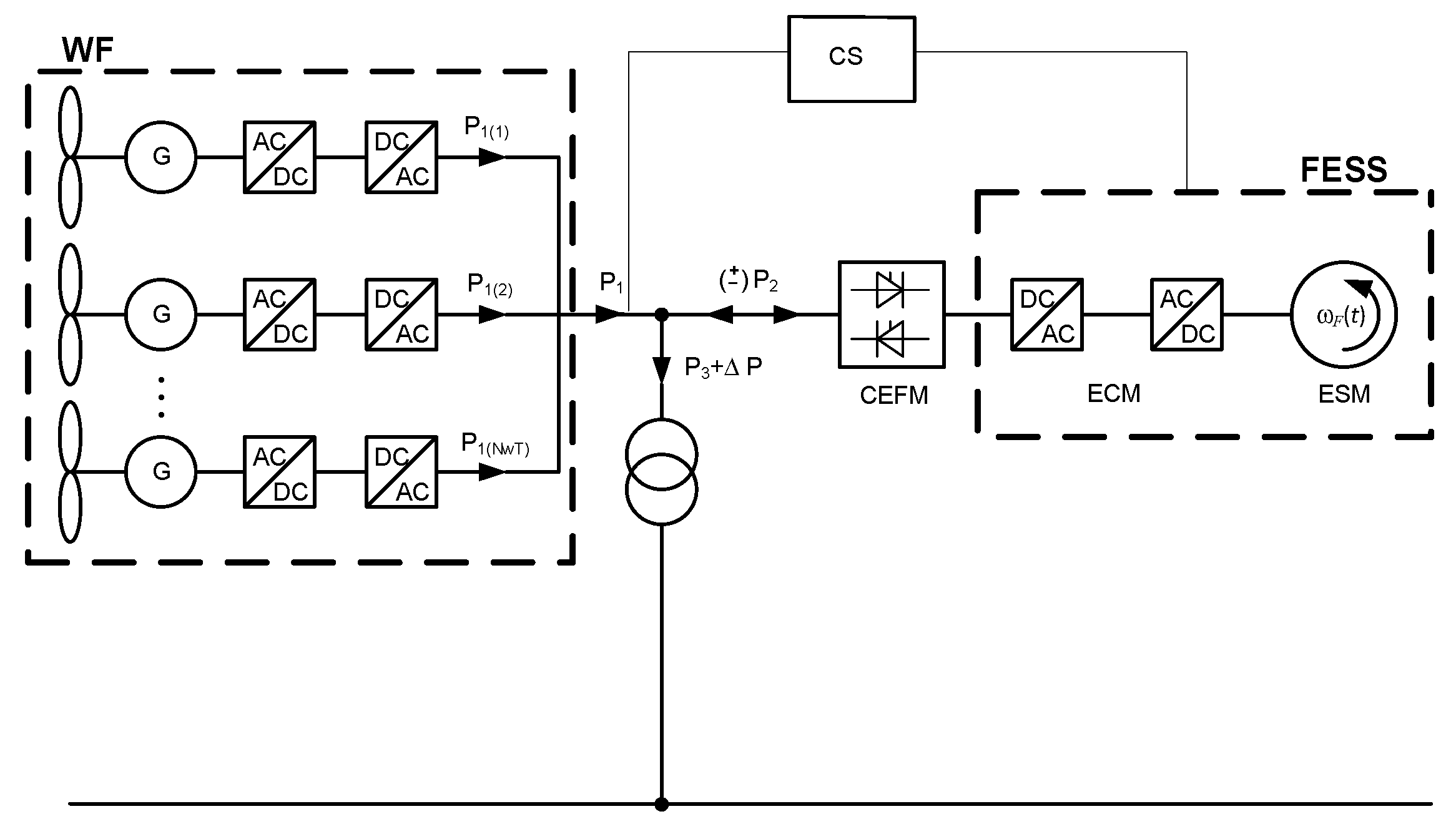
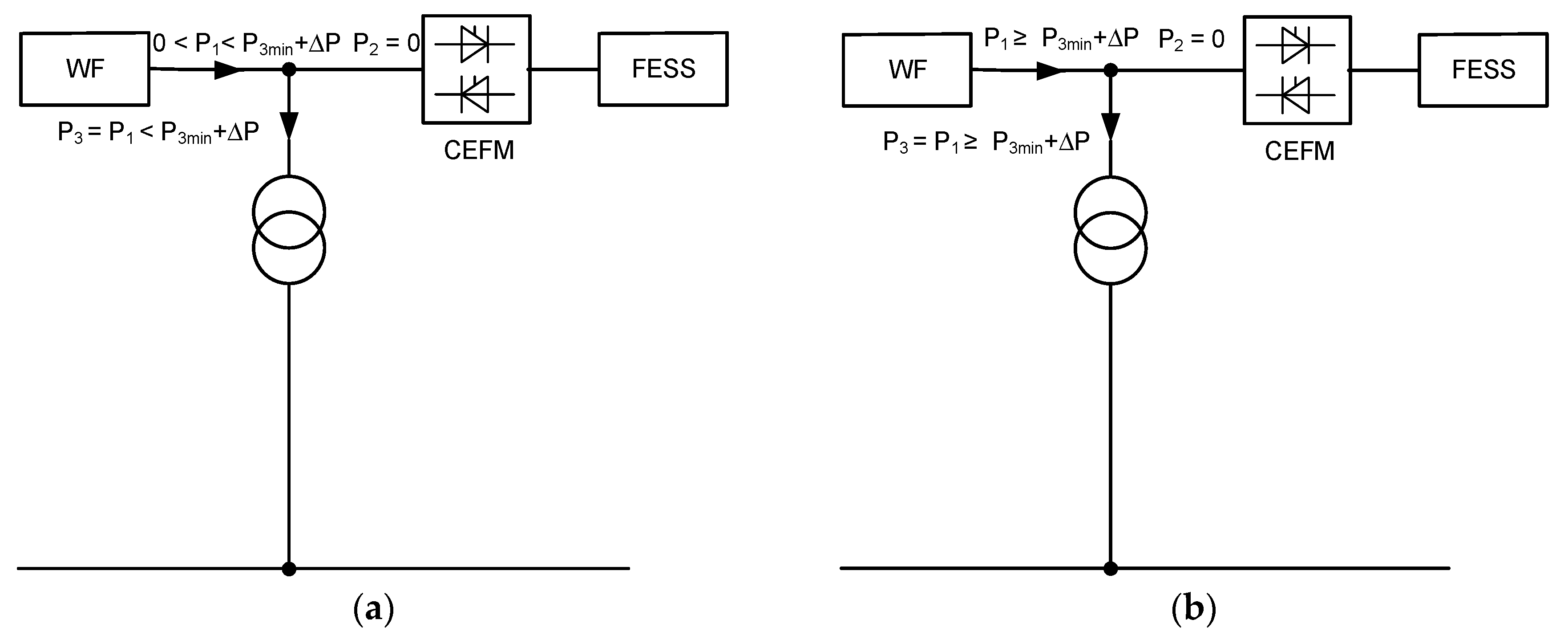
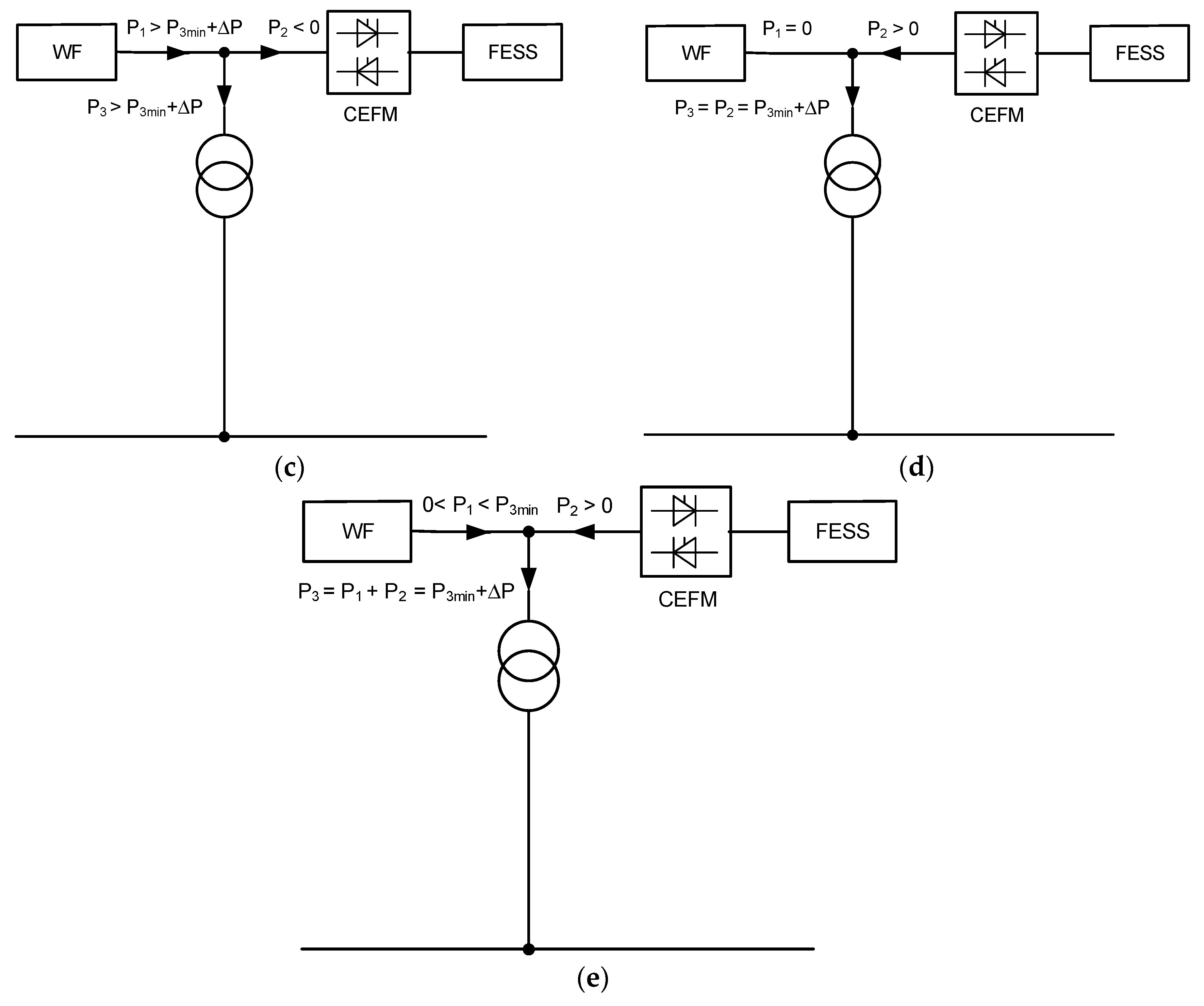
2.1. Description of the System, Power Flow Algorithm

A wind farm is an unstable source with random values of the instantaneous power P1(t) in the range [0, PWFn], where PWFn stands for the total of the rated power values of all turbines. The annual and multi-annual deterministic components add to the stochastic nature of the wind speed changes, which means that a period of one year should be taken as the minimum period of analysis for such systems.
In relation to the above, even high rated power wind farms, where turbines are located at a certain distance from one another, do not guarantee stable power released to the power grid in either short (minutes) or long (hours, days) time intervals [16]. The stability and predictability of power generation by the sources within the power grid are essential in order to guarantee an adequate level of power supply reliability and determine the energy safety of a country. In the case of wind sources, the best results of the output power stability (power released to the power grid) are achieved by using energy storage devices with a capacity suited to the power plant efficiency, its geographical location and assumed period of continuous operation. The capacity of the storage not only depends on the farm’s efficiency and the mean annual wind speed vwAvg, but also on the dynamics of wind speed changes specific for the local conditions, and on the statistical parameters of breaks in power generation: their mean duration, the number of subsequent intervals between the periods when the energy storage can be charged, etc. The author has presented detailed results of such studies in Reference [24].
Figure 1 presents a schematic diagram of a wind farm cooperating with a global (common for all turbines) storage of kinetic type. The power generated in each turbine P1(i)(t) (for i = 1, 2, …, NWT, where NWT is the number of turbines in the farm) is supplied to a node and then—depending on the instantaneous power of farm P1 and the state of charge (SOC) of the ESS—to storage P2 and/or power grid P3. The storage can also operate with power P2 when discharged, and then the stored energy is supplied to the power grid. The (+) sign of power P2 means that the storage is discharged, while (−) stands for its charged conditions. Power P3 is supplied to the power grid. The power is the sum of the power of the turbines and the storage, reduced by the ΔP power loss in the transformer and the line supplying power to the grid:
P 3 ( t ) = P 1 ( t ) + P 2 ( t ,   SOC ) Δ P
The CFEM (control flow of energy module) is responsible for controlling the flow of energy between the wind farm, storage, and power grid.
It is possible to improve the reliability of electrical energy supplies to the power grid from a wind farm-kinetic energy storage system when an appropriate control algorithm is implemented that stores the flow of energy between the turbines, storage and power grid.
This assumes that the minimum set power P3min on the system outlet is maintained at all times with the maximum duration Tmax, even when the wind speed drops below the turbine cut-in speed vcut-in (then P1 = 0). At an appropriately selected energy storage capacity AFESSn [24], it is possible to recover power in the periods when the power generated by the farm is lower than the assumed minimum value P3min. In this way, the system guarantees the maintenance of power supplied to the power grid regardless of weather conditions in a period not longer than Tmax and with power not lower than P3min. The implementation of energy storage results in an increase in the predictability of the source generation related to the partial stabilisation of its output power P3.
From the point of view of the acquired functionalities of the system presented in Figure 1, the control system is among its most important elements. The control system responds to the instantaneous values of wind speed vw(t) and the storage charging level SOC(t). Considering the turbine cut-in speed (vcut-in), reaching the rated power (vn) and the output power of the farm P3min (v3min), turbine cut-out time (vcut-out) and the generated power values corresponding to them, one can identify four operating conditions of a wind farm-kinetic energy storage system: independent operation of the farm, storage charging, independent operation of the storage and simultaneous operation of the storage and farm. The conditions and system diagrams corresponding to them are presented in Figure 2. The arrows mark the energy flow directions that depend on the current wind speed, the acquired power level P3min, the capacity of AFESSn storage and its charging level, as well as the mutual relations between power P1, P2max, P3, and P3min, where P2max is the maximum power of storage.

2.2. Wind Speed Measurement Data

A simulation of the operation of the system described in Section 2.1, establishing the course of instantaneous power, generated power, and the impact of a kinetic energy storage system on the reliability of electrical energy supplies to the power grid, requires the use of data which characterise the wind conditions. Measurements of the wind speed were used for this paper. Each sample represented the mean wind speed in the period ΔtM ≈ 47 s, while the number of samples used for one year was to 670,000. The duration of the kth sample is expressed based on the formula tk = k∙ΔtM, for k = 1, 2, …, N, where N stands for the number of samples.
All measurements used in the paper were carried out with an NP-3 (Far Data) anemometer in the radiation transfer station in Strzyżów near Rzeszów—south-eastern Poland at a height of hM = 10 m AGL. The reference measurement data were re-calculated for the actual altitude of the turbine nacelle hWT, for the needs of the study, according to the relationship describing the exponential form of the vertical profile of wind speed changes [25]:
v WT ( t k ) = v wM ( t k ) ( h WT h M ) α
where: k is wind speed sample number, vWT is wind speed at the height of the wind turbine nacelle hWT, vwM is wind speed at the measurement height hM, and α is coefficient depending on the land roughness.

3. Mathematical Model of the System

3.1. Turbine and Wind Farm

The identification of a turbine output power by means of an analysis, based on the wind speed measurement values requires the use of a mathematical and numerical model of the turbine [25]. In order to examine the reliability of power supplies from the wind farm to the power grid, a simplified model was used for the wind speed sampling period ΔtM. In the simplified model, the wind turbine plays the role of a functional unit modelling the power characteristics P1 = f(vw(t)). Based on linear interpolation between two points of the turbine power’s discrete characteristics, the power generated for the kth sample of the wind speed vw (tk) can be identified based on the following formula:
P 1 ( v w ( t k ) ) = { P 1 + P 2 P 1 v 2 v 1 ( v w ( t k ) v 1 )   for   v cut - in v w ( t k ) < v wn P WTn   for   v wn v w ( t k ) v cut - out 0   for   other   v w ( t k )
where: v1, v2 are wind speed values on the discrete characteristics of the turbine power between which the speed v1vw(tk) ≤ v2 is positioned, P1 and P2 correspond to the wind speed, v1 and v2 are turbine power values read from discrete power characteristics.
In order to approximate the farm model to its actual operating conditions, differences in the position and, hence, the actual wind speed on the nacelle level were taken into consideration for each NWT turbine. To that end, random changes (±5%) in the wind speed (in the moment tk) were considered for each turbine as compared to measurement samples. Thus, for the ith turbine and kth sample, the wind speed (in the moment tk) is:
v w ( i ) ( t k ) = ( 1 ± r n d   ( 0.05 ,   0.05 ) ) v w ( t k )
where: rnd (−0.05, 0.05) is a random value (normal deposition) from the [−0.05, 0.05] range. Then, the power released to the power grid from the reference farm is:
P 3 ( t k ) = i = 1 N WT P 1 ( i ) ( ( 1 ± r n d   ( 0.05 ,   0.05 ) ) v w ( t k ) ) Δ P

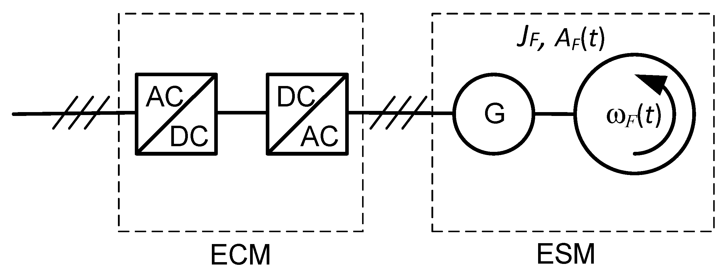
3.2. Kinetic Energy Storage

Kinetic energy storage systems use an indirect method of electrical energy storing in the form of flywheel rotational kinetic energy. Its shape, material and maximum rotational speed determine the storage dimensions, capacity, and weight, and are simultaneously the basic criteria of their division [9,24,26,27,28]. Figure 3 presents a general construction diagram of a kinetic energy storage system using a three-phase AC machine.
Analyses carried out to identify the reliability of power supply to the power grid do not require the consideration of all aspects of kinetic storage modelling and, especially, of dynamic states. A change in the storage charging level as a function of time (subsequent wind speed measurement samples) is important for the issue in question. Therefore, storage modelling was limited to the following equation of the rotational movement dynamics:
J F d ω F d t = P 2 ω F + ω F K 1 + K 2
where: JF is the moment of inertia of the system, P2 is the storage charging/discharge power, ωF is the rotational speed of the rotor, K1 is the coefficient of friction, K2 is the Coulomb’s friction.
Solving Equation (6), when the storage capacity, dimensions of the rotational mass and scope of changes in the working speed and efficiency of electrical systems, which are part of the storage, are known, one can identify the course of changes in the power stored in the storage system when it is connected to a wind turbine and power grid, and execute the algorithm given in Section 2.1.

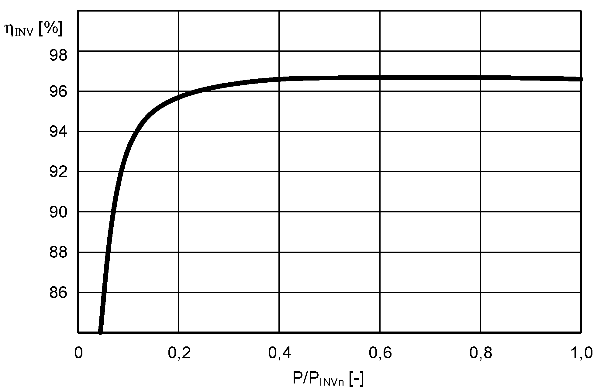
3.4. Power Electronics Systems Controlling the Flow of Power

From the point of view of the executed algorithm (point 2.1), power electronics systems related to DC electrical energy conversion into AC and vice versa (in the kinetic storage structure) and control of the energy flow between the turbine, storage and power grid according to Equation (1), are all important elements of the system presented in Figure 1. The efficiency of the abovementioned systems is a parameter that greatly affects the effectiveness of power conversion. A typical relationship of a power electronics converter ηINV as a function of load ηINV = f (P/PINVn) is used in the acquired model, where P is converted power, and PINVn is the rated power of the converter assembly. Figure 4 presents the assumed efficiency characteristics of power electronics systems.

4. Indicators of Electrical Energy Supplies from a Wind Farm—Kinetic Energy Storage System to the Power Grid

An assessment of electrical energy generation reliability for the assumed period involves the identification of the extent to which power demand Pz(t) is covered by the capacity of subsystem Pw(t). Information about reliability established for future periods (e.g., following changes in the structure of the interesting part of the grid) includes load connection, additional unstable sources etc. A model of power generation reliability, as a difference in the value of stochastic processes Pz(t) and Pw(t), is also defined as a stochastic process D(t) which is a power deficit. This is described by the general relationship [29]:
D ( t ) = { P z ( t ) P w ( t )   for   P z ( t ) > P w ( t ) 0   for   P z ( t ) P w ( t )
Indicators related to the duration of power deficit, power not supplied to customers and frequency and duration of occurrence, loss of energy expectation (LOEE), frequency and duration indices (F&D), expected capacity deficiency (ECD), probability of capacity deficiency (PCD), expected loss of load (XLOL) etc.—are used as quantitative parameters describing a stochastic process of a power deficit D(t) [29,30,31,32,33].
A method based on an analysis of the changes in the level of the output power P3 for a one-year period was used to compare the reliability of electrical energy supplies to the power grid from a wind farm—kinetic energy storage system with various structures. The application of an energy storage system helps to shape the changes in the power supplied to the system as compared to the power level resulting from changes in the wind energy. The applied indicators are similar to the parameters defined for a power deficit stochastic process D(t) but they still take into consideration the acquired power flow control algorithm (Section 2.1). Furthermore, they are identified based on historical data. The following indicators are used further in this paper:
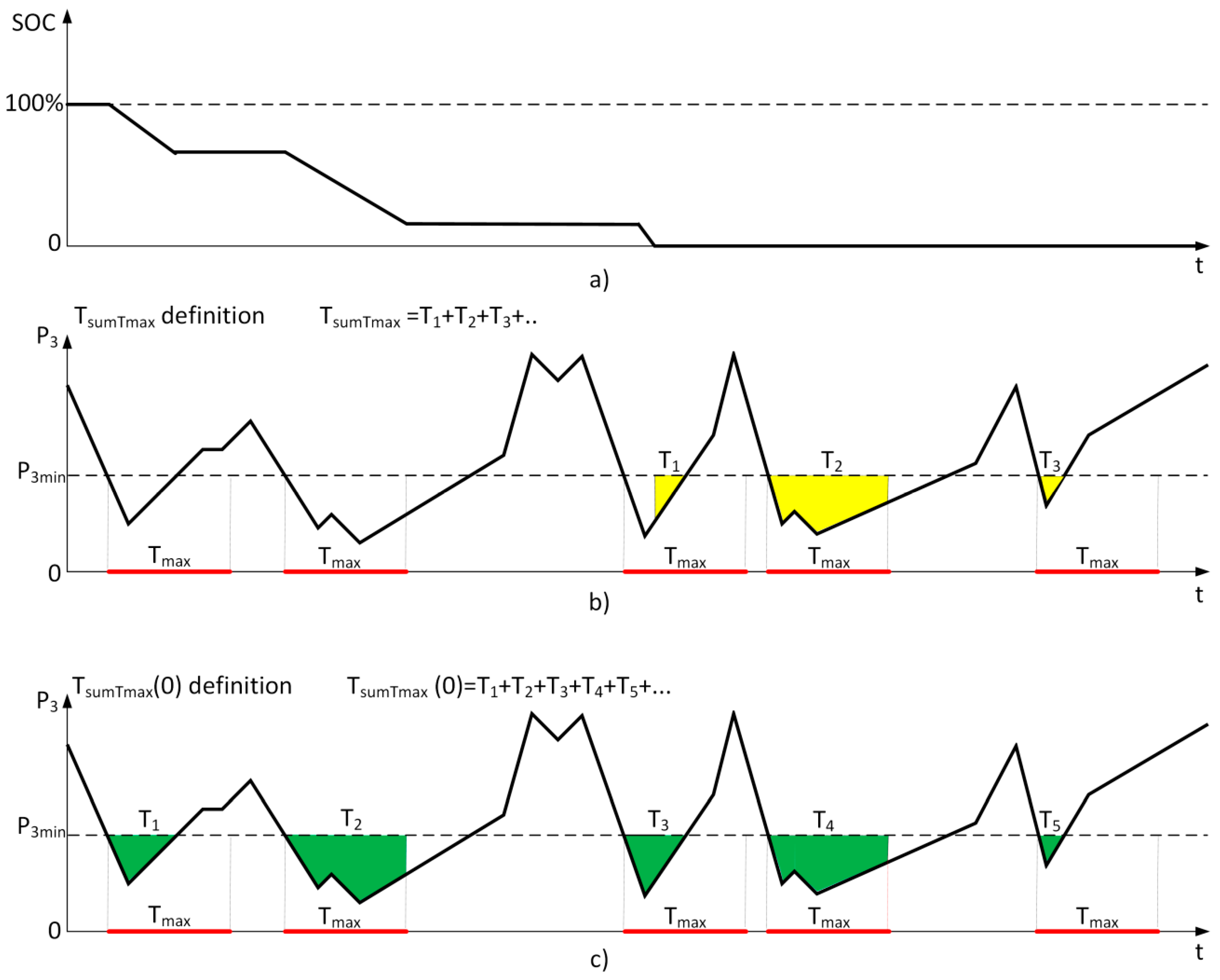
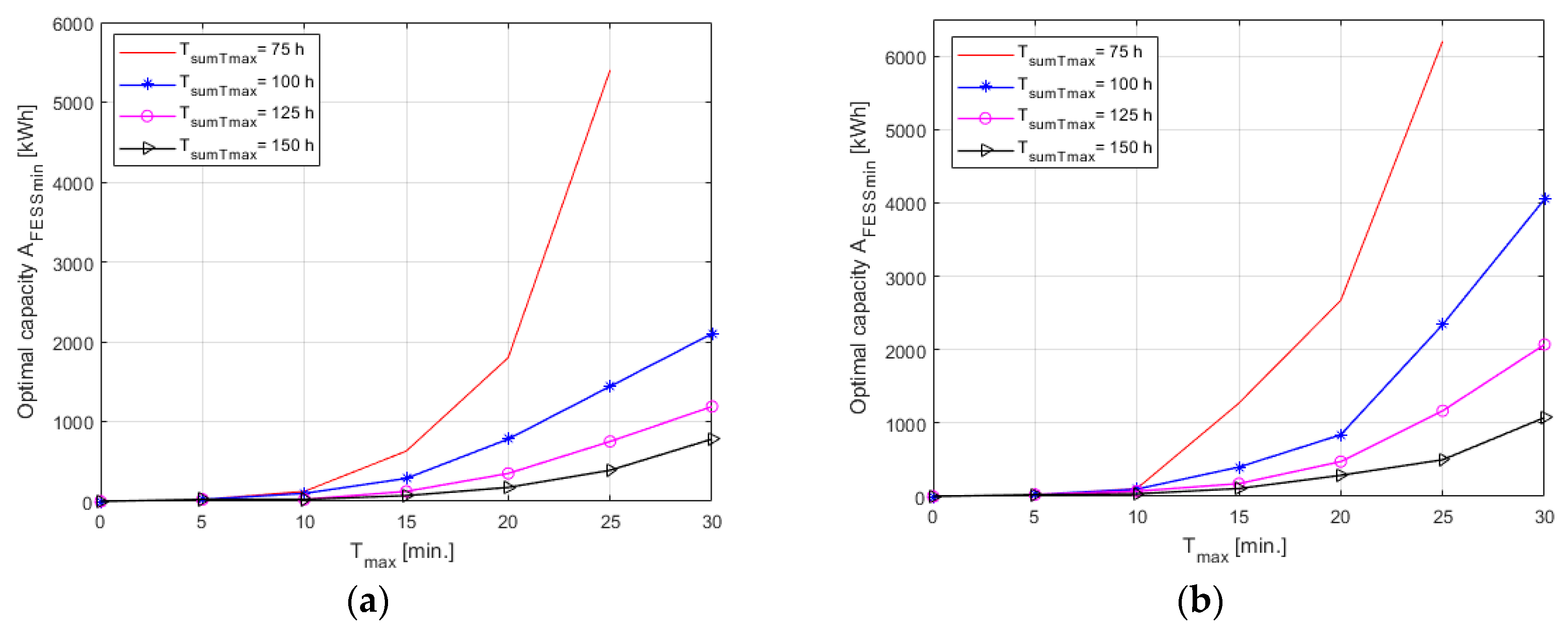
  • total annual time of power generation with a value lower than P3min, covering only the periods lasting up to Tmax (according to the system operation algorithm, the generated power deficit is replenished by the energy from the storage) at the storage capacity AFESS:
    T s u m T m a x ( A F E S S ) = i = 1 M T T m a x ( i )
    where: TTmax(i) is the duration of the ith interval which is shorter than or equal to Tmax in which the power supplied to the grid P3 is lower than the assumed minimum power P3min, and M is the number of intervals TTmax in which power deficit occurs,
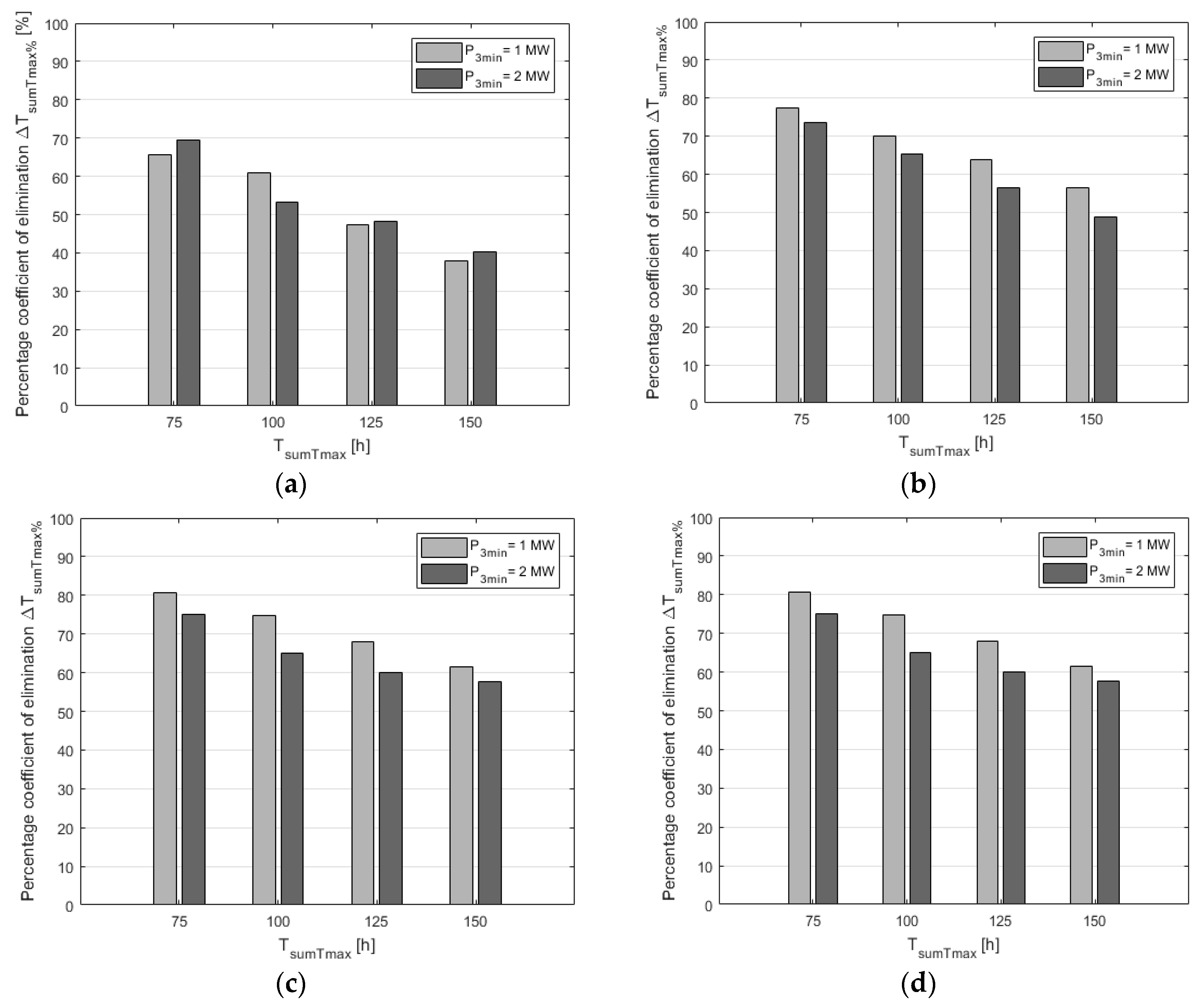
  • percentage coefficient of elimination of periods when the generated power value is lower than P3min, considering only the periods which last up to Tmax:
    Δ T s u m T m a x % = T s u m T m a x ( 0 ) T s u m T m a x ( A F E S S ) T s u m T m a x ( 0 ) × 100 %
    where: TsumTmax(0) is time TsumTmax identified for a system without storage, TsumTmax(AFESSn) is the time TsumTmax identified for a system with energy storage with a rated capacity AFESS (the diagram explaining the difference between Tmax, TsumTmax and TsumTmax(0) was presented in Figure 5),
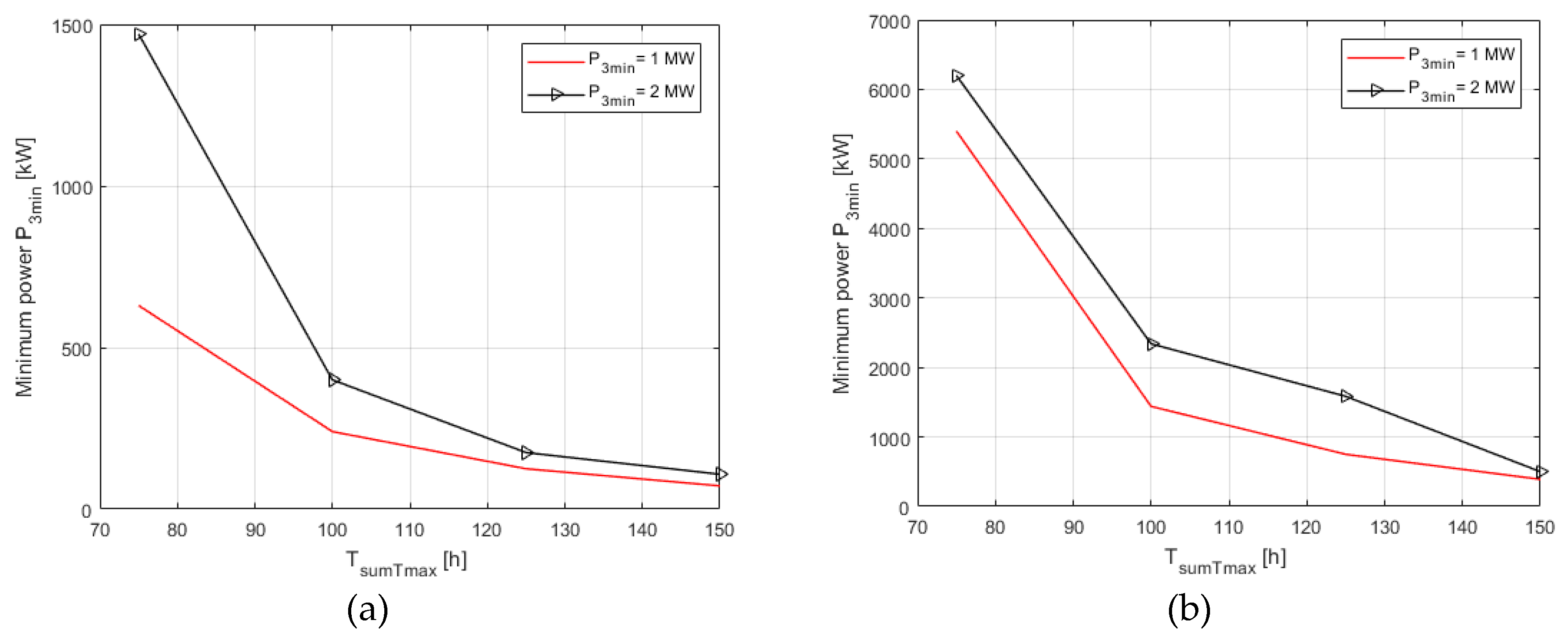
  • power deficit accounting only for periods lasting up to Tmax:
    Δ A = i = 1 M T T m a x ( i ) ( P 3 m i n P 3 a v g ( i ) )
    where: P3avg(i) is the mean power supplied to the grid from the wind farm—kinetic energy storage system in the ith interval shorter than or equal to Tmax, in which the power released to the grid P3 is lower than the assumed minimum power P3min.
Equation (8) identifies the total time composed of periods no longer than Tmax, in which the deficit of power generated by the system (P3 < P3min) was not completely covered by the energy in the storage. Efforts are made to minimise the indicator, while its value close to zero means complete elimination of power outages in the assumed maximum duration Tmax. High values of Equation (9) mean elimination of the majority of outages with duration up to Tmax. Efforts are then made to keep the value at 100%. Equation (10) characterises the system operation on the power side and helps to identify the power which was not supplied to the power grid in periods lasting up to Tmax. Efforts are made to keep the value of Equation (10) as low as possible, and ideally at 0.

5. Optimisation of a Wind Farm—Kinetic Energy Storage System

5.1. Purpose of Optimisation, Function and Constraints

The purpose of the optimisation task solved in the paper is to identify the structure of a wind farm—kinetic energy storage system, which for the set rated power of the farm PWTn and its geographical location minimises the capacity of AFESS storage limiting the annual time of supplies of power values to the power grid below P3min (considering only the periods which last up to Tmax) to TsumTmaxY. The vector of decisive variables x includes: wind turbine type NWT (x1), turbine height hWT (x2), number of turbines nWT (x3), type of kinetic storage NFESS (x4), and the number of connected energy storage modules nFESS (x5). The minimisation task defined in this way takes the following form:
A ˙ F E S S = min { A F E S S ( x ) } = f ( N WT ,   n WT ,   h WT ,   N F E S S ,   n F E S S ,   w )
where: A ˙ F E S S is the minimum capacity value meeting the requirements for the set operating conditions of the system, as w is the collection of algorithm parameters of energy flow between the farm, storage, and power grid.
The type of turbine used (variable x1) determines its power curve and at the same time the power generated in the moments specified by available wind speed samples. In the case of turbine, several variants are available differing in the installation height of the rotor (variable x2), which, according to Equation (2) to the vertical profile of wind speed variations, also affects the level of power generated by the turbine. The number of turbines specified by the variable x3 allows obtaining the nominal power of the PWFn farm assumed in the algorithm. With the assumed minimum power P3min (definition in Section 2.1), the number and duration of periods of power generation by the farm below the level P3min depend on the variables x1, x2 and x3 in Figure 5. Individual modules of kinetic magazines are characterized by different energy capacities, but the most important from the point of view of the analysed problem are the values of their maximum charging and discharging power (these parameters are determined by the variable x4). The last of these parameters in various ways adapt the properties of the energy storage in the field of exchange the energy, to the real dynamics of wind speed changes at a specific farm location (the course of changes in wind speed). The last variable x5 affects the total capacity and power of the used kinetic energy storage system.
Equation (11) can be solved only when considering the collection of constraints, i.e., the relationships (equality and/or inequality) which identify the size of the acceptable solution area X. Structural constraints in the analysed task (related directly to the vector of decisive variables) expressed in a standardised form include:
  • True power of the farm PWFr(x):
    1 P W F r ( x ) 0.9 P W F n 0 P W F r ( x ) 1.1 P W F n 1 0
  • Size of turbine database (number of designs and turbine heights) and kinetic storage units (number of energy storage types).
Constraints in the true power of the farm PWFr(x) are related to the inclusion in the calculation process of a finite collection of turbine designs whose multiple power values are not always equal to the assumed rated power of the farm PWFn.
Functional constraints (not related to vector x) cover the parameters which are a result of a numerical analysis of the system operation (output power P3) and are related to characteristic indicators of the control algorithm of the energy flow between the farm, storage, and power grid. In the analysed task, the functional constraints in a standardised form cover:
  • time TsumTmax(x) − Equation (6):
    T s u m T m a x ( x ) T s u m T m a x 1 0
    where: TsumTmaxY is the total annual boundary time of power generation below P3min assumed in the optimisation task, covering only the periods lasting up to Tmax;
  • maximum power of kinetic storage PFESSMax(x):
    1 P F E S S M a x ( x ) P 3 m i n 0
Interrelations between the parameters of the selected turbine (power characteristic, height) and a single module of energy storage (rated energy capacity, maximum charging and discharging power) directly affect, for the given location (wind conditions), the TsumTmax parameter in Figure 5. Equation (13) of limiting the indicated parameter to the value of TsumTmaxY therefore requires the use of different storage capacities for various types of turbines and energy storage. Therefore, the parameters determined in Equation (11) determine the value of the energy storage capacity, and the application of the optimization algorithm described in the paper allows the determination of the optimal structure of the wind farm—kinetic energy storage, minimizing the capacity of the storage working in it, while fulfilling all technical requirements for the cooperation of the farm with power system.

5.2. Selection of Optimisation Method, Description of Application Developed

The selection of the optimisation method dedicated to the solution defined in Section 5.1 of the task requires a detailed analysis of several elements, including in particular: the form of the function of the objective, the number of decisive variables and the size of the acceptable solution area [25,34,35,36]. Additionally, one should consider the possibilities of including in the optimisation complex numerical calculations used for identifying the value of the function of the objective and constraint control. The experience of the authors in the effective use of the method to solve similar tasks is very important [37].
The multi-modal nature of the acquired function of Equation (11) requires the use of stochastic methods or heuristics in order to seek its global extreme. Even though only five variables were defined in the reference task, the task remains complex and time-consuming, as a result of the multiple identification of changes in the power value in the analysed system, the integer nature of decisive variables and the hidden occurrence of variables in the criterion function. In relation to the above, a genetic algorithm population method is used to optimise the structure of a wind farm-kinetic energy storage system, which leads to the minimisation of storage capacity AFESS, according to the system operation algorithm described in Section 2.1. An important advantage of the method is related to its ability to modify the basic parameters in order to improve its effectiveness when performing detailed tasks. A disadvantage in the case of tasks with highly complex calculations is the reduced reproducibility of the results [35,36]. It is also necessary to perform initial tests whose results help to identify the appropriate AG parameters that would improve the reproducibility of the results and reduce calculation time.
The effectiveness of the proposed method in solving tasks of global optimisation in the area of electrical engineering and renewable energy was proven in a number of scientific publications, e.g., [38,39] and the authors used it successfully to optimise the structure of complex electrical light systems, the shape and parameters of high-power lines, and to minimise the cost of power generation in hybrid generation systems [37,40,41,42,43,44,45].
Based on the mathematical model described in Section 3 and a selected optimisation method in Matlab (Lincence no: 975466, Version 2014b, Poznan University of Technology, Poznan, Poland, 2014) and MS Visual Studio environment, an application was developed intended to optimise the structure of a wind farm—kinetic energy storage system with a view to minimising energy storage capacity. The application uses proprietary structures and classes related to different types of energy storage, wind turbines, PV modules, power electronics systems and indicators of the reliability of power supplies to the power grid mentioned in Section 4, as well as functions from the Global optimisation toolbox of the Matlab environment to implement the modified genetic algorithm method.
The assessment of the quality of solutions obtained through optimisation required an analysis of power: generated by farm P1, energy storage P2, and supplied to the power grid P3 in the analysed system. To that end, measurements of the wind speed in a one-year period and data from wind turbines and PV modules collected in a database developed for the purpose of the application were used.
The Augmented Lagrangian Genetic Algorithm (ALGA) interior penalty function method [46] was employed to consider the constraints of the optimisation tasks (Equations (12)–(14)). The ALGA method was implemented in the Matlab environment.

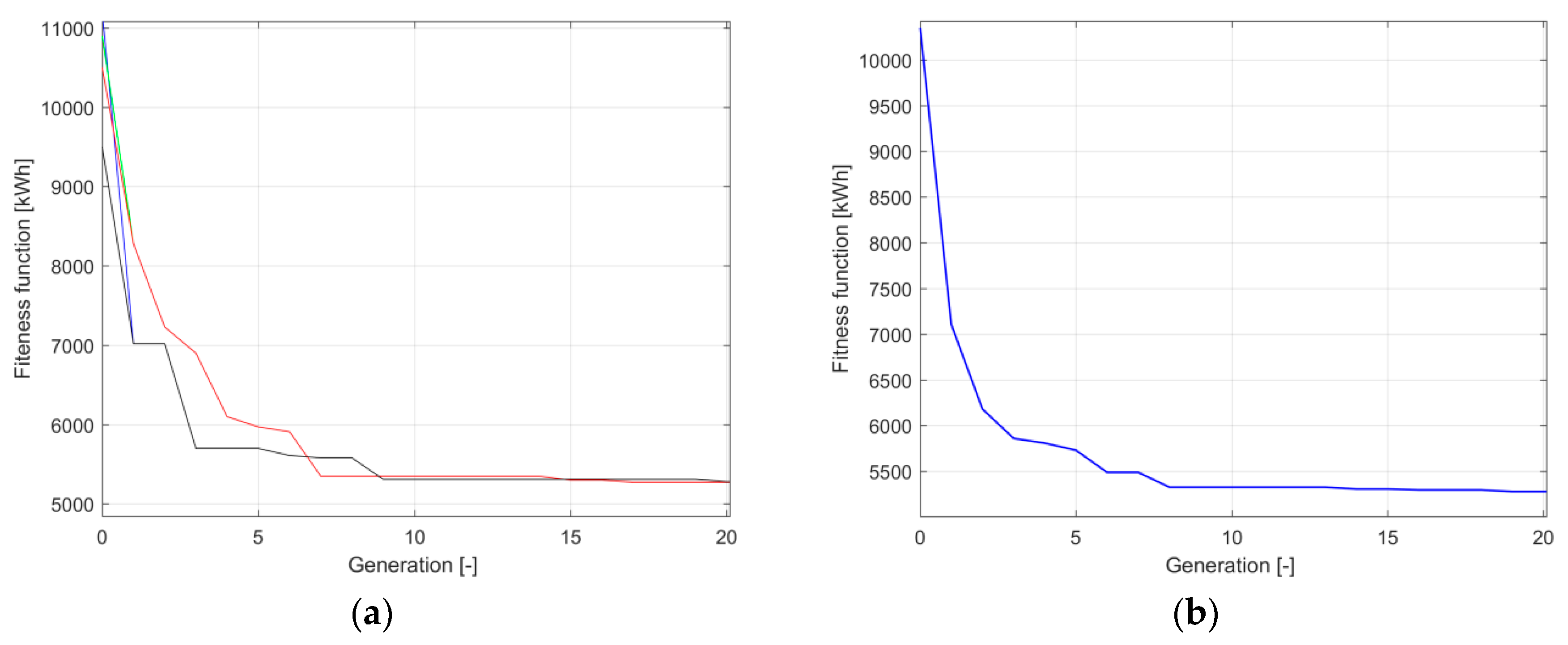
5.3. Optimisation Calculations

A search for the structure of a wind farm—kinetic energy storage system which minimises the capacity of energy storage AFESS (Equation (11)) for the assumed output parameters of the system, was carried out for wind farms with two power values: PWFn(1) = 5 MW and PWFn(2) = 10 MW (indices expressed as integers stand for a parameter option). Six time values were taken into account concerning power generation periods with power values below P3min: Tmax(1) = 5 min, Tmax(2) = 10 min, Tmax(3) = 15 min, Tmax(4) = 20 min, Tmax(5) = 25 min and Tmax(6) = 30 min; two minimum power values P3min(1) = 10%PWFn, and P3min(2) = 20%PWFn; and four values of the acceptable total time: TsumTmax(1) = 75 h, TsumTmax(2) = 100 h, TsumTmax(3) = 125 h, and TsumTmax(4) = 150 h.
The calculations were carried out using the developed optimisation algorithm and application described in Section 5.2 in order to conduct a preliminary study involving changes in the AG parameters to solve the test task. The obtained results helped to draw conclusions relating to the value of the algorithm parameters which contribute to the final solution before the maximum number of iterations, and reduce computing time to ca. 3 h. Finally, a genetic algorithm was applied using the remainder selection method, the Gaussian mutation and elite strategy with a transfer of three best individuals. The number of individuals Np = 50 and the number of generations Ng = 50 were established experimentally.
Figure 6 presents the changes in the value of the best individual’s (solution) adaptation as a function of the generation number for five activations of the algorithm (Figure 6b) for a farm with rated power PWFn(2) = 10 MW, power P3min(2) = 20%PWFn = 2 MW, Tmax(5) = 25 min, and TsumTmax(1) = 75 h.
Figure 7 presents the results of optimisation calculations as changes in the minimum capacity of a kinetic storagesystem which meets the required parameters of a system controlling the flow of energy between the farm, storage and power grid as a function of time Tmax for two wind farms with power PWFn(1) = 5 MW (Figure 7a) and power PWFn(2) = 10 MW (Figure 7b). In each case, the calculations were made for two minimum power values P3min(1) = 10%PWFn and P3min(2) = 20%PWFn and TsumTmax(1) = 100 h.
An essential issue for the analysed class of systems is to identify the relationship between the minimum capacity of the storage AFESSmin and the time of eliminated outages Tmax depending on the maximum total time TsumTmax. Optimisation calculations representing the aforementioned task were performed for a farm with power PWFn(2) = 10 MW, two power values P3min(1) = 10%PWFn = 1 MW and P3min(2) = 20%PWFn = 2 MW and four times TsumTmax:TsumTmax(1) = 75 h, TsumTmax(2) = 100 h, TsumTmax(3) = 125 h and TsumTmax(4) = 150 h. The results (value of the minimum capacity of energy storage AFESSmin meeting the assumed algorithm of the system operation as a function of time Tmax) are presented in Figure 8a (P3min(1) = 10%PWFn = 1 MW) and 8b (P3min(2) = 20%PWFn = 2 MW).
Figure 9 presents the relationship between the minimum capacity of the storage unit AFESSmin and the maximum total time TsumTmax for two values of time Tmax(3) = 15 min and Tmax(5) = 25 min.
Details of the optimisation results of the wind farm-kinetic energy storage system for rated power PWFn(2) = 10 MW and selected parameters P3min, TsumTmax, and time Tmax are presented in Table 1.
Figure 10 presents the changes in the percentage value of the coefficient of elimination of power generation periods with power values below P3min for solutions optimum as a function of time TsumTmax for two power values P3min(1) = 10%PWFn and P3min(2) = 20%PWFn, and two time values Tmax(3) = 15 min (Figure 9a) and Tmax(4) = 20 min (Figure 9b). The data were developed based on information given in Table 1.

5.4. Discussion

Following a thorough analysis of the results it was concluded that the applied optimisation methods, the parameters of the control algorithm of the energy flow between a wind farm, energy storage system and the power grid, and the system model were correct for the characteristics of the analysed task. Its solution had high reproducibility in minimising the capacity of the kinetic storage AFESSmin (Figure 6a) and fast computation times (Figure 6b). In the analysed examples, the tasks were solved between the 30th and 40th generations.
Based on the completed studies, it was established that the relationship between the minimum capacity of the energy storage system AFESSmin meeting the required criteria of a wind farm—kinetic energy storage system and time Tmax was non-linear (Figure 7 and Figure 8). It was demonstrated that the dependence points AFESSmin = f(Tmax) could be approximated by polynomial functions of order 3. The values of the determination coefficients identified for the functions amount to over 0.97, confirming the good fit of a polynomial model for the calculation points. A non-linear character was also observed for changes in the capacity AFESSmin as a function of the optimisation time constraint TsumTmaxAFESSmin = f (TsumTmax) (Figure 9).
The application of higher constraints (lower values of TsumTmax) amounting to 150, 125, 100, and 75 h/year contributed to an increase in the required capacity of energy storage AFESSmin. The increase was diversified for different values of time Tmax and power P3min, but between subsequent values of TsumTmax it usually ranged from 1.5 to 3.0 times (Figure 8). In the case of optimising calculations made for time Tmax = 30 minutes and the strongest constraint TsumTmax = 75 h, the task was not solved (Figure 8) for neitherpower P3min = 10%PWFn nor for P3min = 20%PWFn. Tests were repeated many times and an additional detailed analysis of the system operation with optimised parameters (type and number of turbines) was performed with a simultaneous increase in the power storage capacity. It was demonstrated that TsumTmax could not be limited at the level of 75 h/year by further increasing storage capacity. This was caused by the characteristics of the annual changes in wind speed for the reference geographical location (especially for the mean annual wind speed, which amounts to 4.1 m/s at an altitude of 1 m AGL, and to 6.2 m/s at 100 m AGL), and the nominal parameters of the analysed turbines and energy storages systems.
Depending on the geographical location of the farm and the parameters of the turbines and storage systems, it is possible that no solutions can occur for different values of time Tmax. Therefore, it is important to identify the maximum value of time for the assumed wind farm power PWFn, location and basic parameters of the system for which elimination of power generation periods with power values below P3min is possible on the TsumTmax level. Still, the developed algorithm and application require significant modifications, alongside additional studies. The authors plan to address this in future works on the cooperation between wind farms and kinetic energy storages.
The level of the guaranteed output power P3min (Figure 7 and Figure 8) in periods lasting up to Tmax greatly affects the minimum energy storage capacity AFESSmin. Before establishing the parameter value, one should analyse the actual wind farm operating conditions, especially its mean working power. Increasing the power P3min above the value results in a significant increment in the required energy storage capacity and may mean that the storage unit cannot be fully charged. Consequently, the system is not able to eliminate all assumed energy deficits lasting up to Tmax and does not meet a certain group of constraints TsumTmax (e.g., Table 1—results for Tmax = 30 min and constraints TsumTmax = 75 h). A lack of solutions for the cases analysed in Table 1 applies to a farm with low mean annual power of ca. 1 MW. In cases where solutions were found, the optimum mean annual power values of the wind farms ranged from about 1.5 MW to 3 MW.
The optimisation of the kinetic energy storage capacity helps to achieve high percentage values of the coefficient of elimination of power generating periods when the power value is below P3minTsumTmax% − Equation (9)) which amount to 40–80% (mean 53%) of the analysed cases depending on the value of time Tmax and constraint value TsumTmax (Figure 10). The value of the indicator ΔTsumTmax% increased as the system operation constraints become more stringent (shorter times TsumTmax), entailing a significant increase in the required storage capacity. When the value of the constraint time is reduced twice (from TsumTmax = 150 h to TsumTmax = 75 h), the optimised values of the energy storage capacity were 5 to 14 times higher, depending on time Tmax.
Values of power not supplied to the power grid ΔA (Equation (10)) in the system operation periods with power below P3min and time up to Tmax, analysed in a one-year period (Table 1), were established for the optimised structures of a farm with a kinetic energy storage system. The power value increased as time Tmax and constraint time TsumTmax increase. In the case of the analysed farm with power PWFn = 10 MW, the values were low (Table 1) compared to the total energy generated in a one-year period and they did not exceed 0.5%.
It should be emphasised that it was possible to achieve the presented results of a wind farm—kinetic energy storage system optimisation due to a short (ca. 47 s) period of wind speed averaging. For a typical value of 10 min, it was not possible to precisely simulate the system cooperation with the power grid due to an approximated analysis of the energy storage operation. In such cases, the results for the minimum energy storage capacity AFESSmin suffered from a much higher error. Based on the authors’ experience in the modelling of energy storage using RES, they suggest that the averaging period of wind speed measurements and other parameters related to power generation in RES—irradiation in particular—should be shorter than the period used currently and should amount to one or a few seconds.

6. Conclusions

The paper presents a new algorithm for identifying the minimum capacity of a kinetic energy storage system which helps to improve (on the assumed level) the reliability indicators of electrical energy supplies from an unstable source (i.e., wind farm) to the power grid. The concept of the method can be transferred onto different types of energy storage and unstable sources. In such a case, the relevant mathematical and numerical models of the system elements need to be replaced and preliminary studies conducted to establish the optimisation algorithm parameters.
The analyses helped to draw an important conclusion concerning changes in the values of reliability of power supplies from a wind farm to the power grid. It is possible to improve the value and stabilise the operation of the wind farm at relatively low capacities of energy storage (in cases of moderate parameters of the analysed system and optimisation constraints). It is still important to take such measures towards the majority of farms located close to one another, as it will help to predict the level of power generated from such sources more precisely. Any increase in the requirements concerning the system operating parameters results in a significant (up to several times) increase in the required capacity of the storage, and hence means higher investment and operating costs.
The authors of the paper focused on an essential matter related to the relative increase in the installed power of unstable sources in the generating systems operating in many countries. The situation causes a stochastic variance of electric power generation. The application of the presented methods and results can help to stabilise the output power of unstable sources at limited costs of necessary investments. Local compensation of temporary power deficiencies by storage system included in the structure of large wind farms helps to limit power transmission losses and to improve the total energy efficiency of the system.

Author Contributions

A.T. and L.K. conceived the base of the paper, discussed the optimization method of wind farm with flywheel energy storage system, elaborated summary. A.T. designed models of power system with wind turbine and energy storage, developed computer system, made calculations, prepared drawings. L.K. analyzed the results of simulation and optimization, provided some valuable suggestions, revised the paper.

Funding

This research was funded by Polish Government, grant number [04/42/DSPB/0431].

Conflicts of Interest

The authors declare no conflict of interest.

References

  1. Trzmiel, G. Determination of a mathematical model of the thin-film photovoltaic panel (CiS) based on measurement data. Eksploat. Niezawodn. 2017, 19, 516–521. [Google Scholar] [CrossRef]
  2. Koh, L.H.; Peng, W.; Tseng, K.J.; Gao, Z. Reliability evaluation of electric power systems with solar photovoltaic & energy storage. In Proceedings of the 2014 International Conference on Probabilistic Methods Applied to Power Systems, Durham, UK, 7–10 July 2014; pp. 1–5. [Google Scholar]
  3. Renewables 2016 Global Status Report. Available online: http://www.ren21.net (accessed on 15 May 2018).
  4. Renewable Energy in Europe—2017 Update. Recent Growth and Knock-on Effects; EEA Report, No 23/2017; European Environment Agency (EEA): Copenhagen, Denmark, 2017. [CrossRef]
  5. Europe 2020 Indicators. Available online: http://ec.europa.eu/eurostat/portal/page/portal/europe_2020_indicators/ (accessed on 15 May 2018).
  6. Kasprzyk, L. Modelling and analysis of dynamic states of the lead-acid batteries in electric vehicles. Eksploat. Niezawodn. 2017, 19, 229–236. [Google Scholar] [CrossRef]
  7. Price, J.E.; Sheffrin, A. Adapting California’s energy markets to growth in renewable resources. In Proceedings of the 2010 IEEE PES General Meeting, Providence, RI, USA, 25–29 July 2010; pp. 1–8. [Google Scholar]
  8. Komarnicki, P.; Lombardi, P.; Styczynski, Z. Economics of Electric Energy Storage Systems. In Electric Energy Storage Systems; Springer: Berlin/Heidelberg, Germany, 2017; pp. 181–194. [Google Scholar]
  9. Amiryar, M.E.; Pullen, K.R.; Nankoo, D. Development of a High-Fidelity Model for an Electrically Driven Energy Storage Flywheel Suitable for Small Scale Residential Applications. Appl. Sci. 2018, 8, 453. [Google Scholar] [CrossRef]
  10. Baghaee, H.R.; Mirsalim, M.; Gharehpetian, G.B.; Talebi, H.A. Fuzzy unscented transform for uncertainty quantification of correlated wind/PV microgrids: Possibilistic–probabilistic power flow based on RBFNNs. IET Renew. Power Gener. 2017, 11, 867–877. [Google Scholar] [CrossRef]
  11. Zheng, D.; Semero, Y.K.; Zhang, J.; Wei, D. Short-term wind power prediction in microgrids using a hybrid approach integrating genetic algorithm, particle swarm optimization, and adaptive neuro-fuzzy inference systems. IEEJ Trans. Electr. Electron. Eng. 2018. [Google Scholar] [CrossRef]
  12. Ding, Y.; Wang, P.; Chang, L.P. Reliability evaluation of electric power systems with high wind power penetration. In Proceedings of the 2009 8th International Conference on Reliability, Maintainability and Safety, Chengdu, China, 20–24 July 2009; pp. 24–26. [Google Scholar]
  13. Sideratos, G.; Hatziargyriou, N. An advanced statistical method for wind power forecasting. IEEE Trans. Power Syst. 2007, 22, 258–265. [Google Scholar] [CrossRef]
  14. Chang, W.Y. A literature review of wind forecasting methods. J. Power Energy Eng. 2014, 2, 161–168. [Google Scholar] [CrossRef]
  15. Kassa, Y.; Zhang, J.H.; Zheng, D.H.; Wei, D. Short term wind power prediction using ANFIS. In Proceedings of the 2016 1st IEEE International Conference on Power and Renewable Energy, Shanghai, China, 21–23 October 2016; pp. 388–393. [Google Scholar]
  16. Zhu, Y.; Zang, H.; Cheng, L.; Gao, S. Output Power Smoothing Control for a Wind Farm Based on the Allocation of Wind Turbines. Appl. Sci. 2018, 8, 980. [Google Scholar] [CrossRef]
  17. Mazzeo, D.; Oliveti, G.; Baglivo, C.; Congedo, P.M. Energy reliability-constrained method for the multi-objective optimization of a photovoltaic-wind hybrid system with battery storage. Energy 2018, 156, 688–708. [Google Scholar] [CrossRef]
  18. Alemany, J.; Kasprzyk, L.; Magnago, F. Effects of binary variables in mixed integer linear programming based unit commitment in large-scale electricity markets. Electr. Power Syst. Res. 2018, 160, 429–438. [Google Scholar] [CrossRef]
  19. Lombardi, P.; Röhrig, C.; Rudion, K.; Marquardt, R.; Müller-Mienack, M.; Estermann, A.S.; Voropai, N.I. An A-CAES pilot installation in the distribution system: A technical study for RES integration. Energy Sci. Eng. 2014, 2, 116–127. [Google Scholar] [CrossRef] [Green Version]
  20. Baghaee, H.R.; Mirsalim, M.; Gharehpetian, G.B. Multi-objective optimal power management and sizing of a reliable wind/PV microgrid with hydrogen energy storage using MOPSO. J. Intell. Fuzzy Syst. 2017, 32, 1753–1773. [Google Scholar] [CrossRef]
  21. Kaviani, A.; Baghaee, H.R.; Riahy, G.H. Optimal sizing of a stand-alone wind/photovoltaic generation unit using particle swarm optimization. Simul. Trans. Soc. Model. Simul. 2009, 85, 89–99. [Google Scholar]
  22. Acuña, L.G.; Padilla, R.V.; Mercado, A.S. Measuring reliability of hybrid photovoltaic-wind energy systems: A new indicator. Renew. Energy 2017, 106, 68–77. [Google Scholar] [CrossRef]
  23. Jiang, X.; Zhang, Z.; Wang, J. Studies on the reliability and reserve capacity of electric power system with wind power integration. In Proceedings of the 2012 Power Engineering and Automation Conference, Wuhan, China, 18–20 September 2012; pp. 1–4. [Google Scholar]
  24. Tomczewski, A. Operation of a Wind Turbine-Flywheel Energy Storage System under Conditions of Stochastic Change of Wind Energy. Sci. World J. 2014, 2014, 643769. [Google Scholar] [CrossRef] [PubMed]
  25. Kaabeche, A.; Belhamel, M.; Ibtiouen, R. Techno-economic valuation and optimization of integrated photovoltaic/wind energy conversion system. Sol. Energy 2011, 85, 2407–2420. [Google Scholar] [CrossRef]
  26. Díaz-Gonzáleza, F.; Sumpera, A.; Gomis-Bellmunta, O.; Villafáfila-Roblesb, R. A review of energy storage technologies for wind power applications. Renew. Sustain. Energy Rev. 2012, 16, 2154–2171. [Google Scholar] [CrossRef]
  27. Fuchs, G.; Lunz, B.; Leuthold, M.; Sauer, D.U. Technology Overview on Electricity Storage; Overview on the Potential and on the Deployment Perspectives of Electricity Storage Technologies; Institute for Power Electronics and Electrical Drives: Aachen, Germany, 2012. [Google Scholar]
  28. Amiryar, M.E.; Pullen, K.R. A Review of Flywheel Energy Storage System Technologies and Their Applications. Appl. Sci. 2017, 7, 286. [Google Scholar] [CrossRef]
  29. Paska, J. Reliability Issues in Electric Power Systems with Distributed Generation. Rynek Energii 2008, 5, 18–28. (In Polish) [Google Scholar]
  30. Glossary of Terms Used in Reliability Standards; NERC: Swindon, UK, 2008.
  31. Power System Reliability Analysis; Application Guide; CIGRE WG 03 of SC 38 (Power System Analysis and Techniques); e-cigre: Paris, France, 1987.
  32. Power System Reliability Analysis; Composite Power System Reliability Evaluation; CIGRE Task Force 38-03-10; e-cigre: Paris, France, 1992.
  33. Reliability Assessment Guidebook, version 2.1; NERC: Swindon, UK, 2010.
  34. Castro Mora, J.; Calero Baro, J.M.; Riquelme Santos, J.M.; Burgos Payan, M. An evolutive algorithm for wind farm optimal design. Neurocomputing 2007, 70, 2651–2658. [Google Scholar] [CrossRef]
  35. Goldberg, D.E. Genetic Algorithms in Search, Optimization and Machine Learning; Addison-Wesley Longman Publishing: Boston, MA, USA, 1988. [Google Scholar]
  36. Michalewicz, Z.; Fogel, D.B. How to Solve It: Modern Heuristics, 2nd ed.; Springer: Berlin/Heidelberg, Germany, 2004. [Google Scholar]
  37. Kasprzyk, L.; Tomczewski, A.; Bednarek, K.; Bugała, A. Minimisation of the LCOE for the hybrid power supply system with the lead-acid battery. In Proceedings of the 2017 International Conference Energy, Enviroment and Material Systems, Polanica-Zdroj, Poland, 13–15 September 2017. [Google Scholar]
  38. Ismail, M.S.; Moghavvemi, M.; Mahlia, T.M.I. Genetic algorithm based optimization on modeling and design of hybrid renewable energy systems. Energy Convers. Manag. 2014, 85, 120–130. [Google Scholar] [CrossRef]
  39. Al-Shamma’a, A.A.; Addoweesh, K.E. Techno-economic optimization of hybrid power system using genetic algorithm. Int. J. Energy Res. 2014, 38, 1608–1623. [Google Scholar] [CrossRef]
  40. Bednarek, K. Electrodynamic calculations and optimal designing of heavy-current lines. Prz. Elektrotech. 2008, 84, 138–141. [Google Scholar]
  41. Bednarek, K.; Nawrowski, R.; Tomczewski, A. An application of genetic algorithm for three phases screened conductors optimization. In Proceedings of the 2000 International Conference on Parallel Computing in Electrical Engineering, Trois-Rivieres, QC, Canada, 27–30 August 2000; pp. 218–222. [Google Scholar]
  42. Bednarek, K.; Jajczyk, J. Effectiveness of optimization methods in heavy-current equipment designing. Prz. Elektrotech. 2009, 85, 29–32. [Google Scholar]
  43. Kasprzyk, L.; Tomczewski, A.; Bednarek, K. Efficiency and economic aspects in electromagnetic and optimization calculations of electrical systems. Prz. Elektrotech. 2010, 86, 57–60. [Google Scholar]
  44. Kasprzyk, L.; Nawrowski, R.; Tomczewski, A. Optimization of Complex Lighting Systems in Interiors with use of Genetic Algorithm and Elements of Paralleling of the Computation Process. In Intelligent Computer Techniques in Applied Electromagnetics, Studies in Computational Intelligence; Wiak, S., Krawczyk, A., Dolezel, I., Eds.; Springer: Berlin/Heilderberg, Germany; New York, NY, USA, 2008; Volume 116, pp. 21–29. [Google Scholar]
  45. Nawrowski, R.; Tomczewski, A. Optimization of overall costs in designing complex lighting systems. Acta Techn. CSAV 2008, 53, 65–79. [Google Scholar]
  46. Conn, A.R.; Gould, N.I.M.; Toint, P.L. A Globally Convergent Augmented Lagrangian Barrier Algorithm for Optimization with General Inequality Constraints and Simple Bounds. Math. Comput. 1997, 66, 261–288. [Google Scholar] [CrossRef]
Figure 1. Schematic diagram of a wind farm cooperating with a kinetic magazine of a global type (CS: control system; ECM: Energy Conversion Module; ESM: Energy Storage Module; FESS: flywheel energy storage system; WF: wind farm).
Applsci 08 01439 g001
Figure 2. Power flow in the wind turbine (WT)-FESS system for different system operating conditions: (a,b) independent operation of a wind farm; (c) storage charging; (d) independent operation of the storage (discharging); (e) simultaneous operation of a wind farm and a storage system (P3′—output power of the system considering power losses ΔP in the transformer and the line).
Applsci 08 01439 g002aApplsci 08 01439 g002b
Figure 3. Structure of kinetic energy storage using a three-phase AC machine (AF: flywheel mechanical energy, G: generator, ωF: rotational speed of the system, JF: moment of inertia of the system (mainly the flywheel), AC/DC, DC/AC: power electronics converters.
Applsci 08 01439 g003
Figure 4. Changes in the efficiency of power electronics systems used in the analysed system as a function of a relative value of converted power (P/PINVn).
Applsci 08 01439 g004
Figure 5. The diagram presenting the difference between Tmax, TsumTmax and TsumTmax(0): (a) FESS’s state of charge; (b) process of output power changes P3 with marked periods shorter than Tmax, in which the system does not provide minimum power P3min; (c) process of changes in output power P3 with marked periods shorter than Tmax, in which the system does not provide minimum power P3min.
Applsci 08 01439 g005
Figure 6. Changes in the value of the function of the best individual’s adaptation as a function of the generation number for a farm power PWFn(1) = 10 MW, power P3min(2) = 20%PWFn = 2 MW, Tmax(3) = 25 min and TsumTmax(1) = 75 h: (a) for five activations of the genetic algorithm; (b) mean value from ten activations of the genetic algorithm.
Applsci 08 01439 g006
Figure 7. Changes in the optimum (minimum) capacity of a kinetic energy storage system AFESSmin as a function of time Tmax for two power values P3min(1) = 10%PWFn and P3min(2) = 20%PWFn and time TsumTmax(x) = 100 h for: (a) a farm with rated power PWFn(1) = 5 MW; (b) a farm with rated power PWFn(2) = 10 MW.
Applsci 08 01439 g007
Figure 8. Changes in the minimum (optimum) capacity of a kinetic energy storage system AFESSmin as a function of time Tmax for a farm power PWFn(2) = 10 MW, time: TsumTmax = 75 h, TsumTmax = 100 h, TsumTmax = 125 h, TsumTmax = 150 h and the optimised system data: (a) P3min(1) = 10%PWFn = 1 MW; (b) P3min(2) = 20%PWFn = 2 MW.
Applsci 08 01439 g008
Figure 9. Changes in the minimum (optimum) capacity of the kinetic storage unit AFESSmin in the function of time TsumTmax for: (a) Tmax(3) = 15 min; (b) Tmax(5) = 25 min.
Applsci 08 01439 g009
Figure 10. Changes in the percentage value of the coefficient of elimination of power generation periods with power values below P3min (Equation 9) for a farm with rated power PWFn =10 MW, power P3min = 1 MW and P3min = 2 MW and: (a) Tmax(2) = 10 min; (b) Tmax(3) = 15 min; (c) Tmax(4) = 20 min; (d) Tmax(5) = 25 min.
Applsci 08 01439 g010
Table 1. Results of optimising calculations for selected configurations of a wind farm—kinetic storage system for a farm with rated power PWFn(2) = 10 MW and different time values Tmax.
No.P3min (MW)Tmax (min)TsumTmax (h)TsumTmax (AFESSmin) (h)TsumTmax(0) (h)ΔTsumTmax (%)AFESSmin (kWh)Turbine’s Number/Power(−)/(MW)PWFnr (MW)ΔA (MWh)
Tmax(2) = 10 min
11107573.7214.365.612510/0.9921.1
211010096.2247.161.0725/1.8931.6
3110125122.5232.147.2364/2.39.238.5
4110150144.8225.537.8256/1.810.847.6
52107573.4241.669.610810 0.9937.3
621010092.7198.053.21004/2.39.249.3
7210125120.5231.248.1723/3960.4
8210150144.2241.540.2366/1.810.872.0
Tmax(3) = 15 min
91157574.9329.877.363012/0.910.825.7
1011510093.3312.270.124010/0.9930.0
11115125118.1327.663.91254/2.39.236.9
12115150142.7327.656.4724/2.39.242.8
132157574.9283.973.614704/2.39.250.9
1421510098.2283.965.44004/2.39.263.4
15215125123.6283.956.41754/2.39.275.6
16215150145.2283.948.91084/2.39.284.5
Tmax(4) = 20 min
171207574.7384.980.6180012/0.910.837.8
1812010099.5397.774.968412/0.910.834.1
19120125123.3384.967.935010/0.9940.3
20120150147.9384.961.617510/0.9946.7
212207574.9302.875.3267011/0.99.952.0
2222010098.8285.665.484010/0.9962.9
23220125124.9314.260.247412/0.910.876.5
24220150149.5353.057.72884/2.39.296.7
Tmax(5) = 25 min
251257574.9447.283.3540010/0.9929.3
2612510099.3482.879.414404/2.39.239.2
27125125124.9447.272.175010/0.9944.0
28125150148.7447.266.839010/0.9954.6
292257574.9355.578.9620011/0.99.954.4
3022510099.8355.571.9234011/0.99.970.3
31225125124.7334.162.7158410/0.9987.3
32225150148.9334.155.550010/0.9995.8
Tmax(6) = 30 min
3313075-------
3413010099.3552.082.121006/1.810.854.0
35130125124.3552.077.511886/1.810.865.0
36130150148.9552.073.07806/1.810.875.9
3723075-------
3823010099.8426.976.6405012/0.910.870.9
39230125124.9398.868.7207011/0.99.988.3
40230150149.7378.960.5107511/0.99103.0

