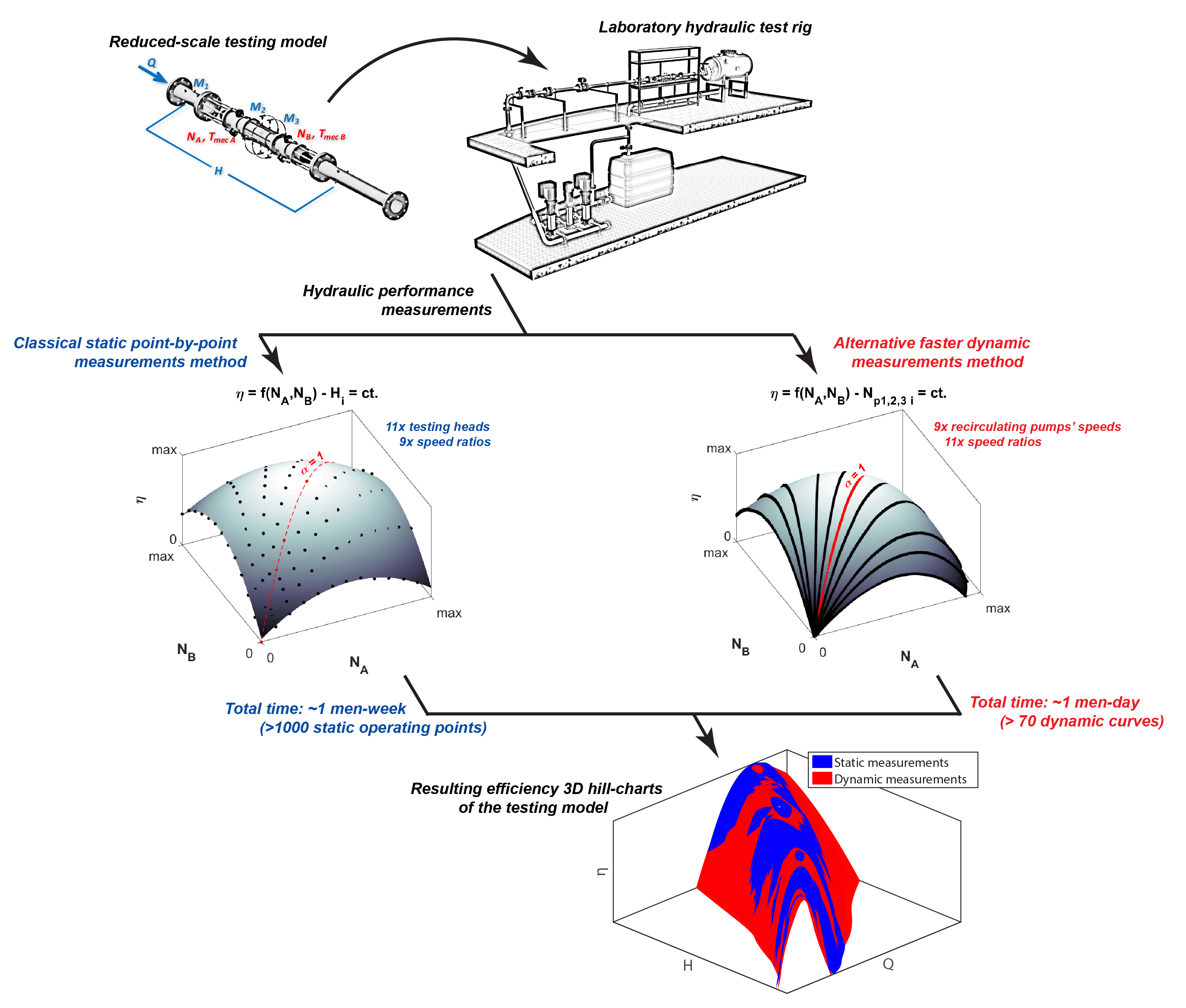
Figure 1.
Standard methodology to reconstruct the full hydraulic efficiency hill-chart of a double-regulated machine using the classical static measurements method: (a) First step: measurements of several efficiency hill-charts at constant testing head Hi and constant speed ratio between the two runners, αi; (b) Second step: calculation of discharge-efficiency and head-efficiency envelopes for all testing heads; (c) Third step: construction of the final full 3D hill-chart of the machine by surface interpolation using the previously obtained envelopes.
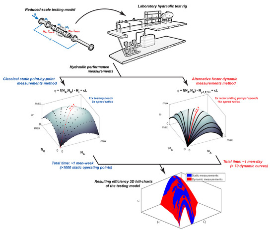
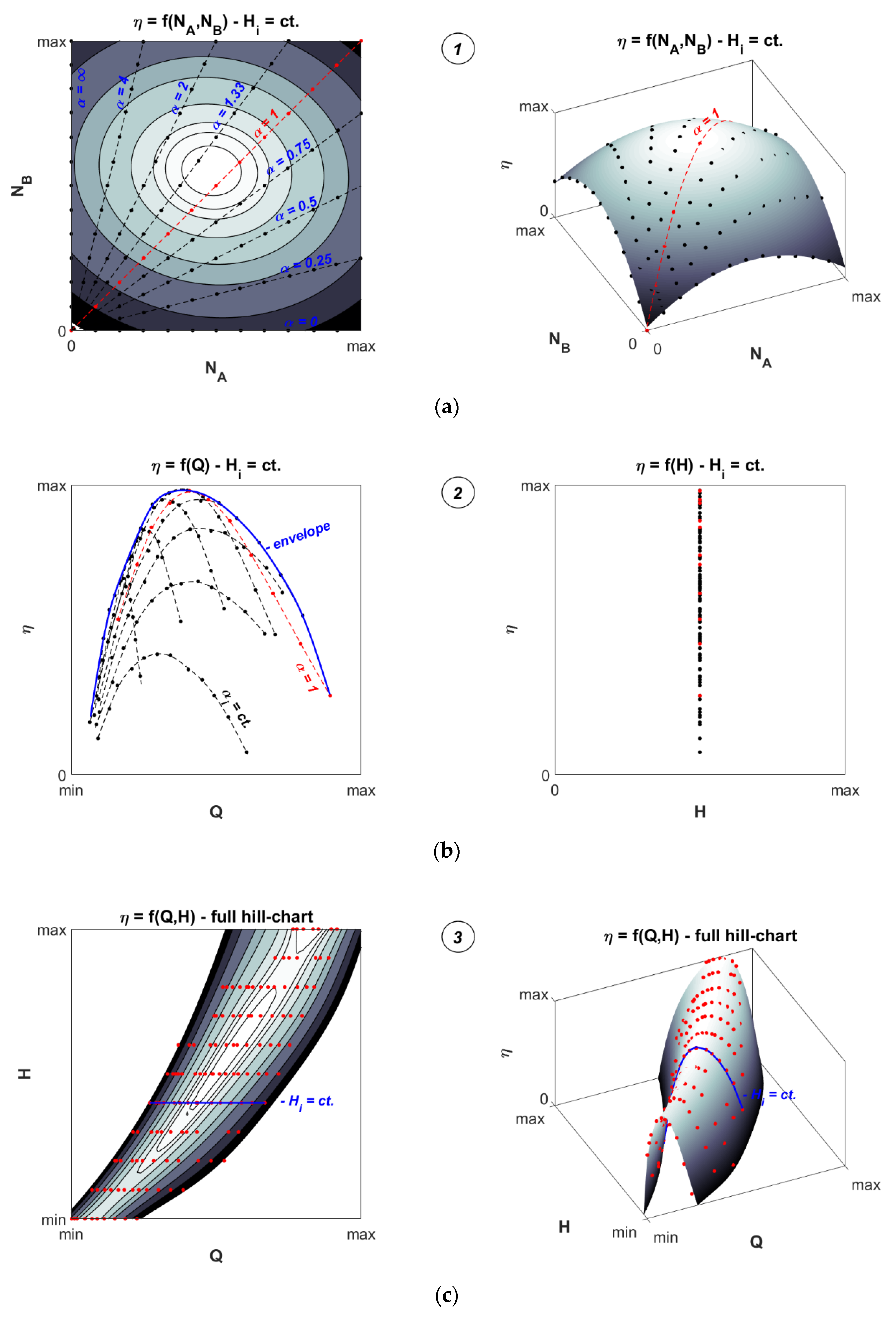
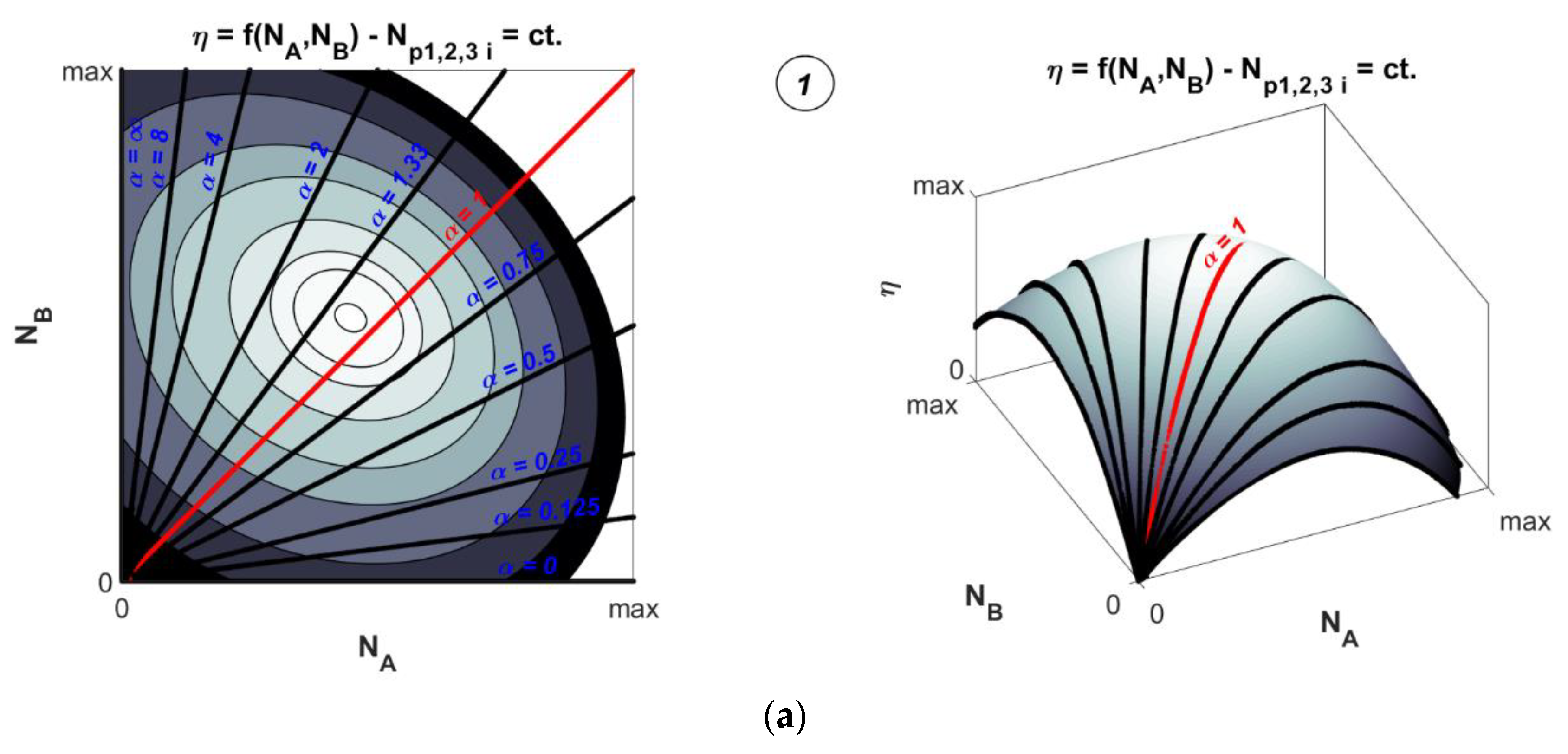
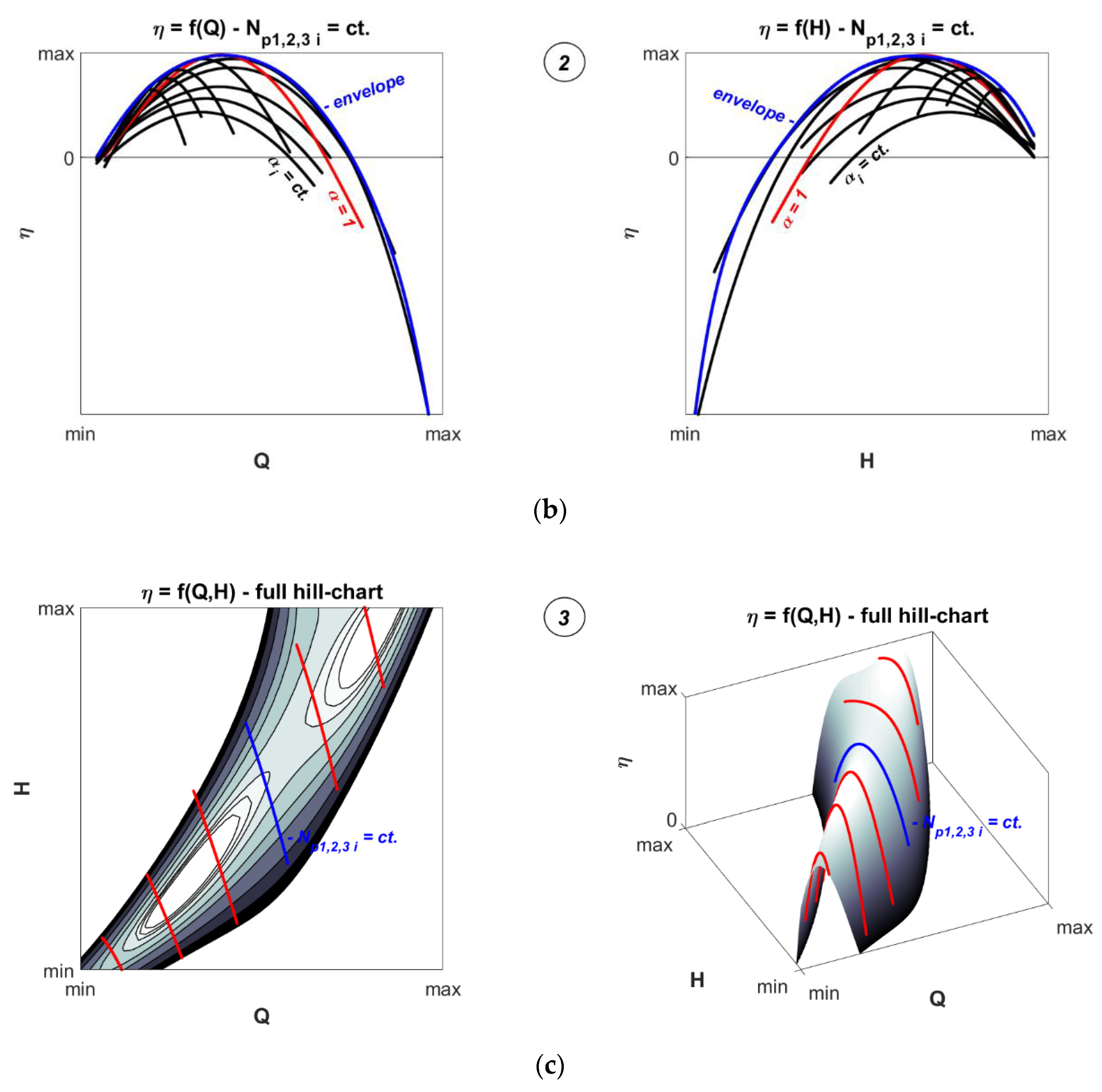
Figure 2.
Employed methodology to reconstruct the full hydraulic efficiency hill-chart of a double-regulated machine using the alternative dynamic measurements method: (a) First step: measurements of several efficiency hill-charts at constant rotational speed Np1,2,3 i of the test rig recirculating pumps and constant speed ratio between the two runners, αi; (b) Second step: calculation of discharge-efficiency and head-efficiency envelopes for all testing recirculating pumps’ speed values; (c) Third step: construction of the final full 3D hill-chart of the machine by surface interpolation using the previously obtained envelopes.
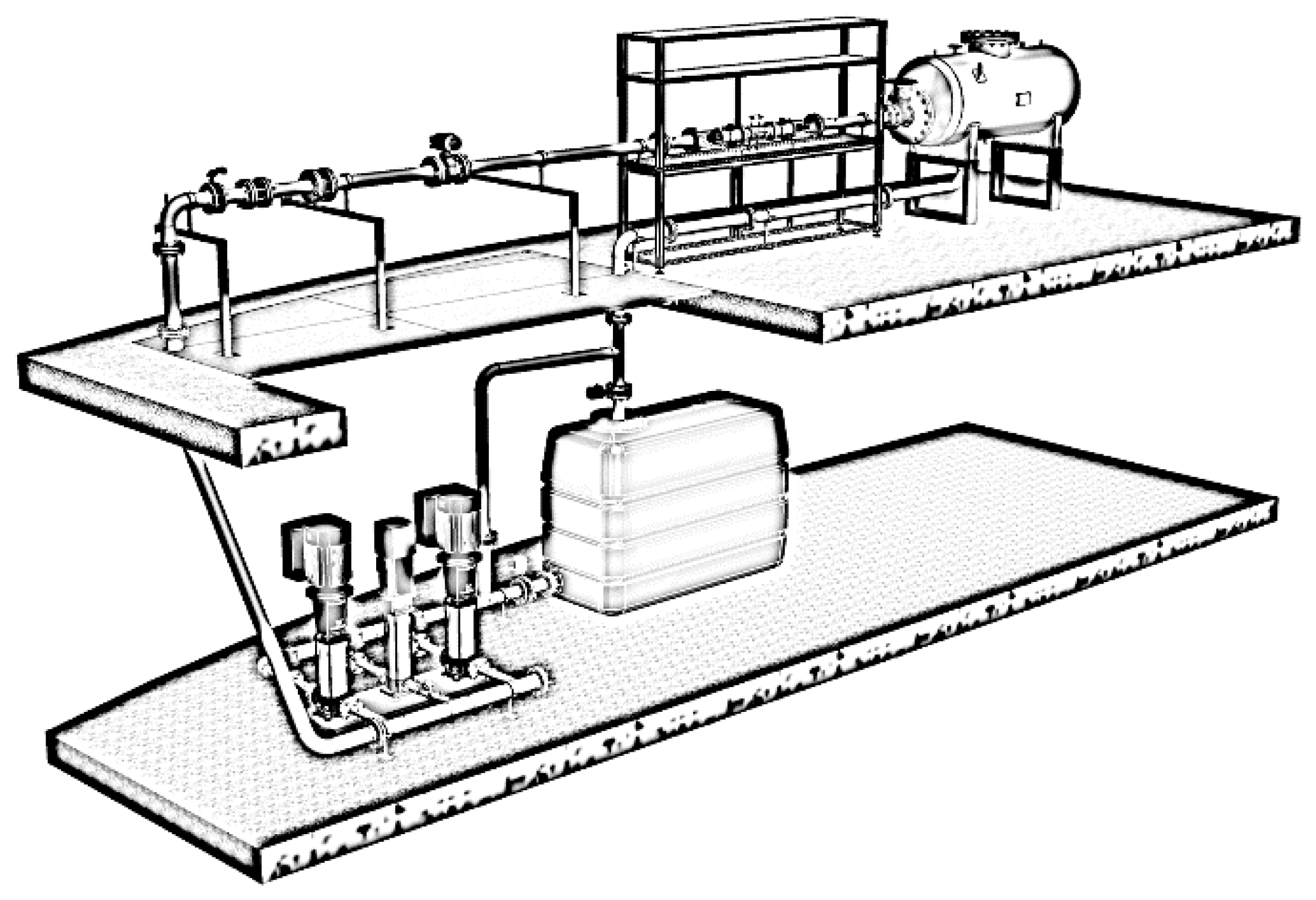
Figure 3.
Hydraulic test rig (2016 version) of the HES-SO Valais//Wallis—Switzerland [
12]. (Main characteristics: (1) Maximum head: 160 mWC; (2) Maximum discharge: ±100 m
3/h; (3) Generating power: 20 kW; (4) Pumping power: 2 × 18.5 kW and 1 × 5.5 kW; (5) Maximum pumps’ speed: 3500/3000 min
−1; (6) Total circuit volume: 4.5 m
3).
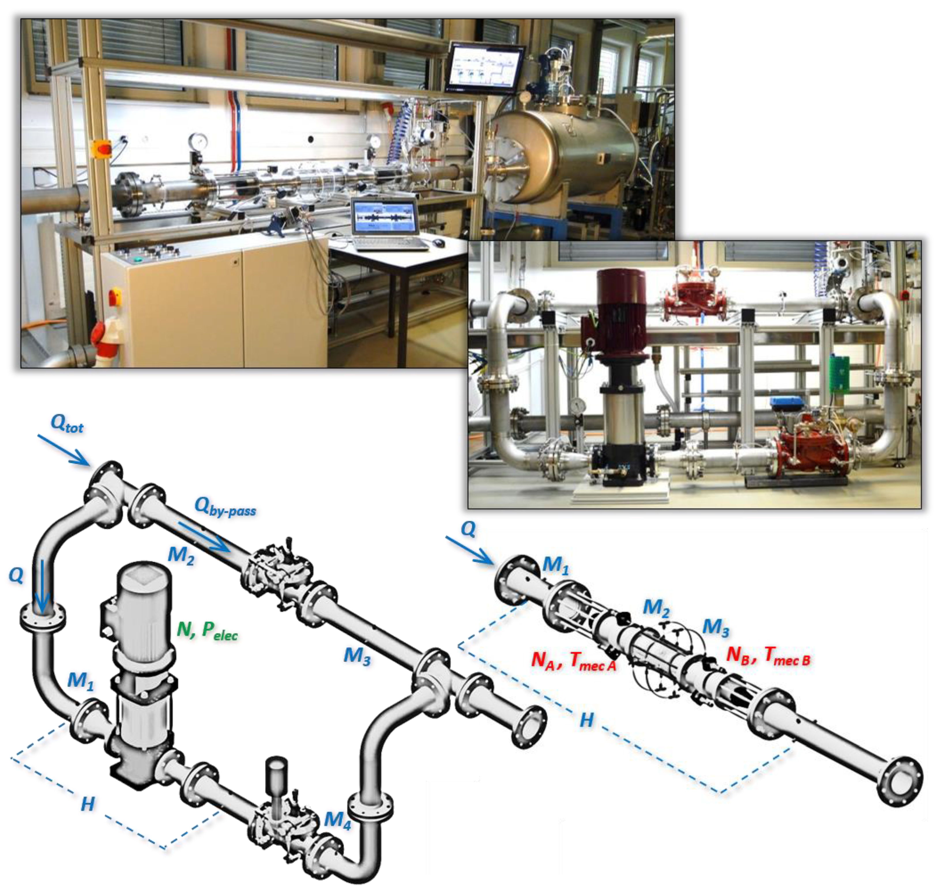
Figure 4.
Experimental setup of the counter-rotating microturbine and of the pump-as-turbine (PAT) for hydraulic performance measurements on the test rig.
Figure 4.
Experimental setup of the counter-rotating microturbine and of the pump-as-turbine (PAT) for hydraulic performance measurements on the test rig.
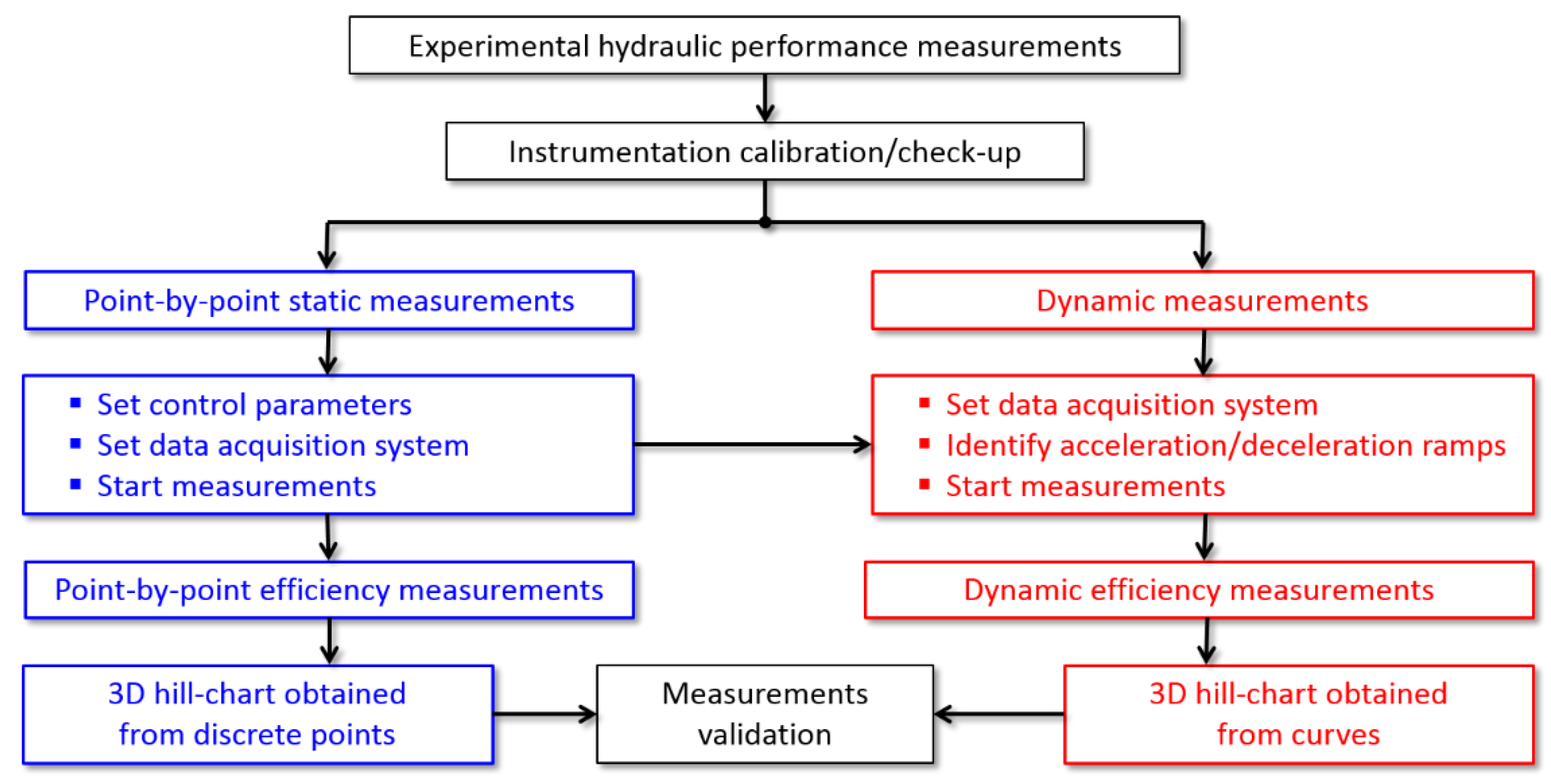
Figure 5.
Flowchart of the employed experimental protocol [
32,
33].
Figure 5.
Flowchart of the employed experimental protocol [
32,
33].
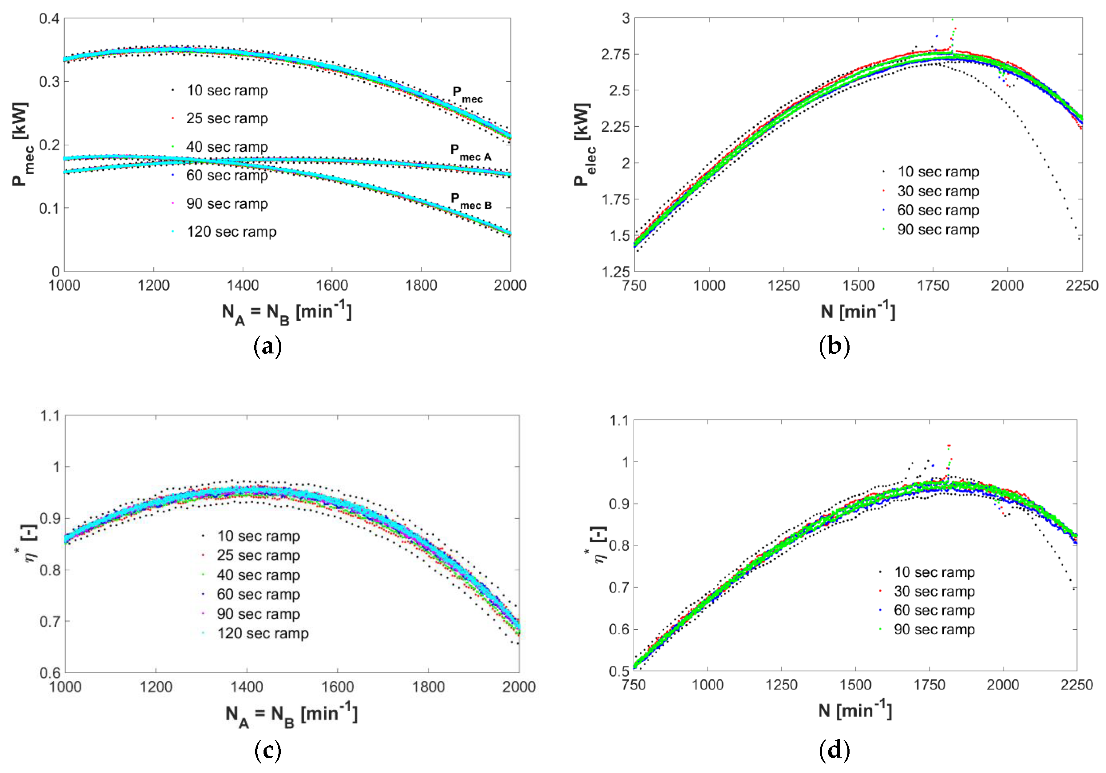
Figure 6.
Influence of the acceleration/deceleration ramp of the runner(s) speed on the power and on the efficiency during one forth and back cycle at fixed testing inflow conditions: (a) variation of the counter-rotating microturbine mechanical power (Np1,2,3 = 1500 min−1); (b) variation of the PAT electrical power (Np1,2,3 = 2000 min−1); (c) variation of the counter-rotating microturbine efficiency (Np1,2,3 = 1500 min−1); (d) variation of the PAT efficiency (Np1,2,3 = 2000 min−1).
Figure 7.
Influence of the acceleration/deceleration ramp of the runner(s) speed on the efficiency fluctuation during one forth and back cycle at fixed testing inflow conditions: (a) counter-rotating microturbine—constant test rig pumps’ speed of Np1,2,3 = 1500 min−1; (b) PAT—constant test rig pumps’ speed of Np1,2,3 = 2000 min−1.
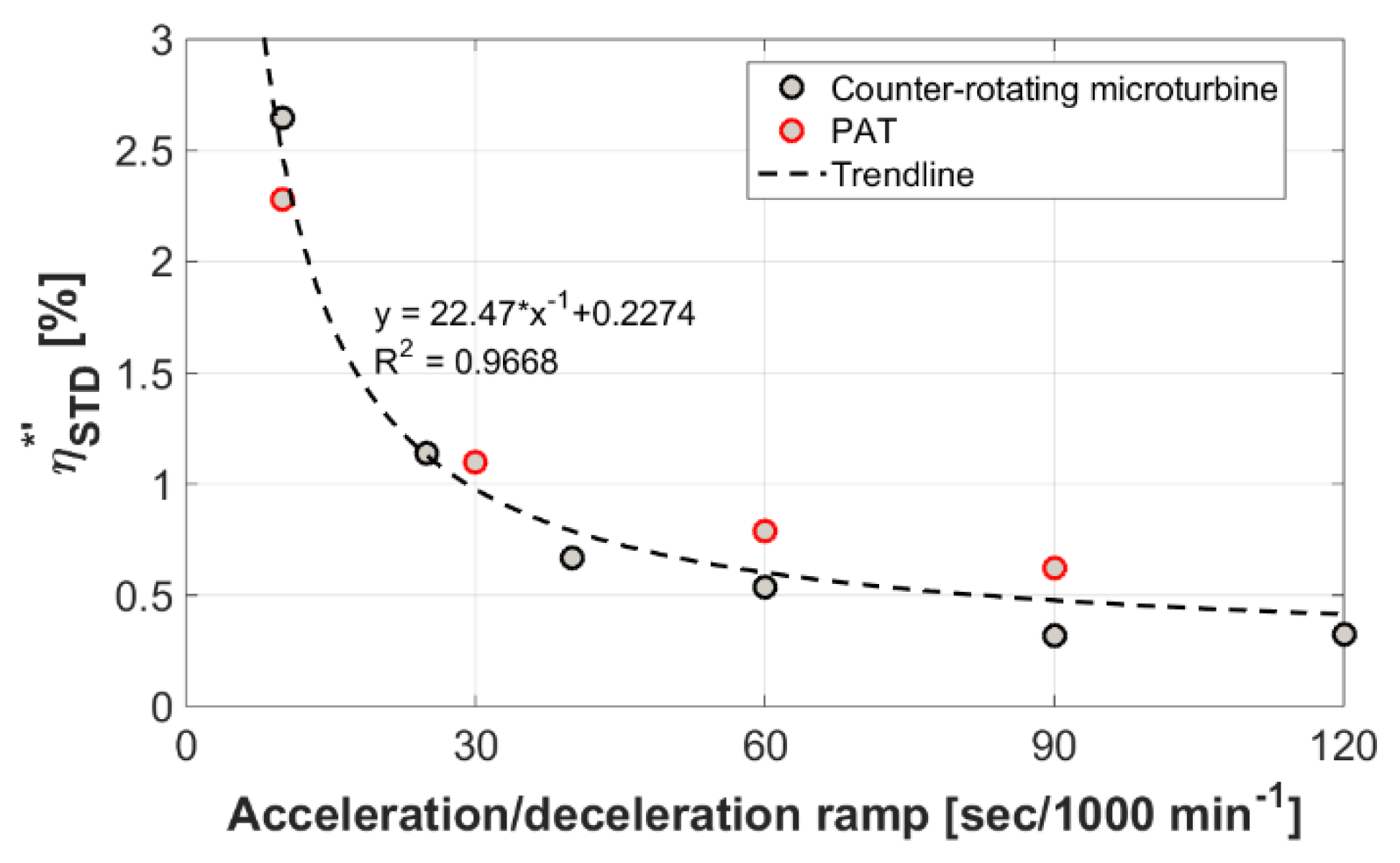
Figure 8.
Resulting efficiency fluctuation standard deviation (STD) depending on the acceleration/deceleration ramp.
Figure 8.
Resulting efficiency fluctuation standard deviation (STD) depending on the acceleration/deceleration ramp.
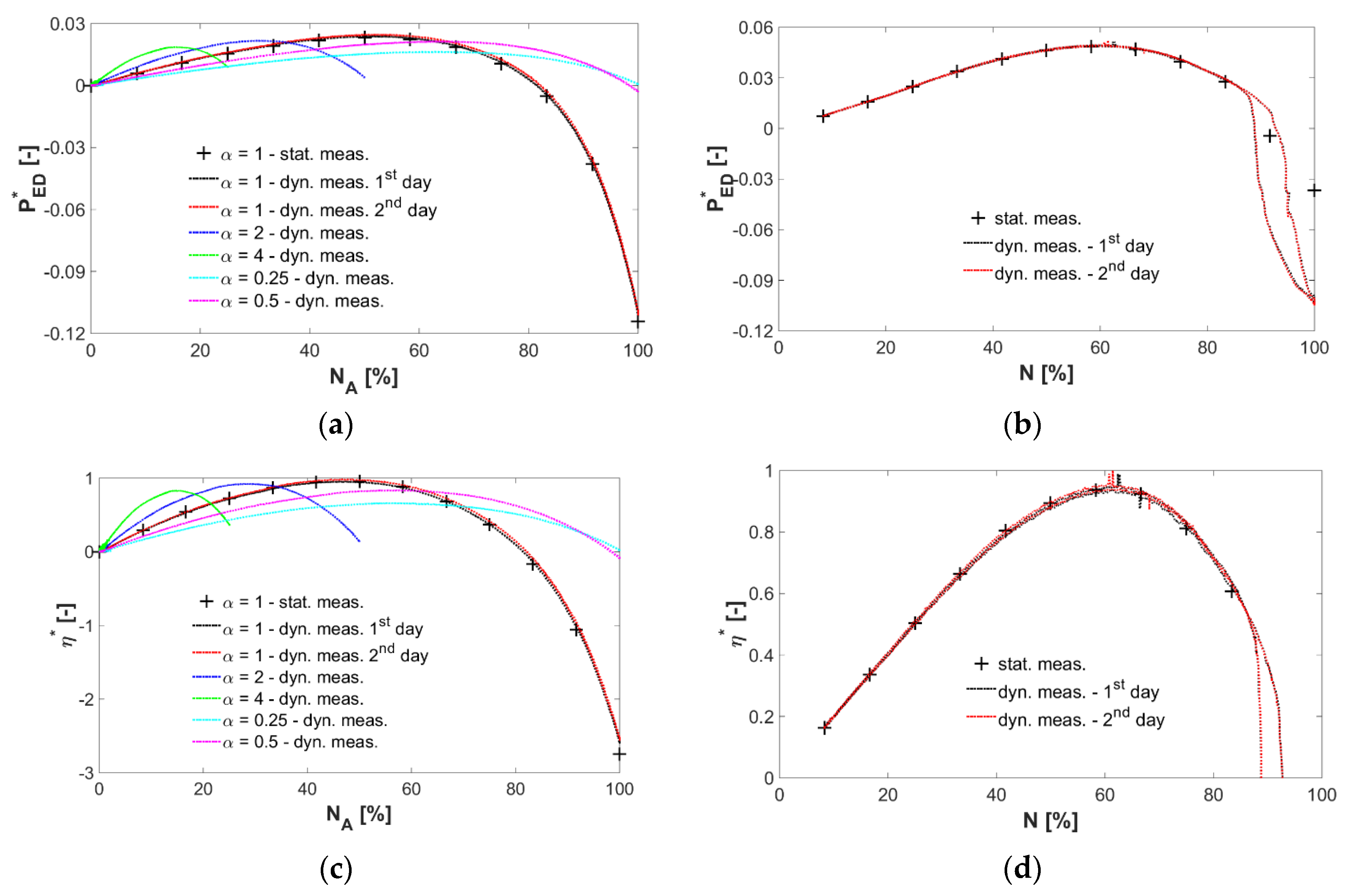
Figure 9.
Dynamic versus static power coefficient and efficiency measurements during one forth and back cycle at fixed testing inflow conditions: (a) variation of the counter-rotating microturbine power coefficient (Np1,2,3 = 1500 min−1); (b) variation of the PAT power coefficient (Np1,2,3 = 2000 min−1); (c) variation of the counter-rotating microturbine efficiency (Np1,2,3 = 1500 min−1); (d) variation of the PAT efficiency (Np1,2,3 = 2000 min−1).
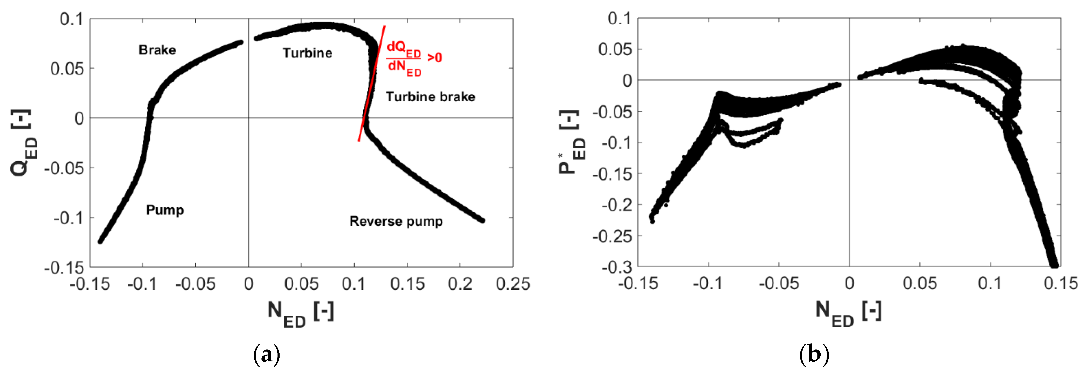
Figure 10.
Resulting 4-quadrant characteristic curves of the PAT obtained by the dynamic measurements method: (a) speed-discharge factor characteristic curve; (b) speed-power factor characteristic curves.
Figure 10.
Resulting 4-quadrant characteristic curves of the PAT obtained by the dynamic measurements method: (a) speed-discharge factor characteristic curve; (b) speed-power factor characteristic curves.
Figure 11.
Resulting efficiency hill-chart contours obtained by classical static point-by-point and by the dynamic measurement methods: (a) counter-rotating microturbine—result of static measurements; (b) PAT—result of static measurements; (c) counter-rotating microturbine—result of dynamic measurements; (d) PAT—result of dynamic measurements; (e) contour plot scale.
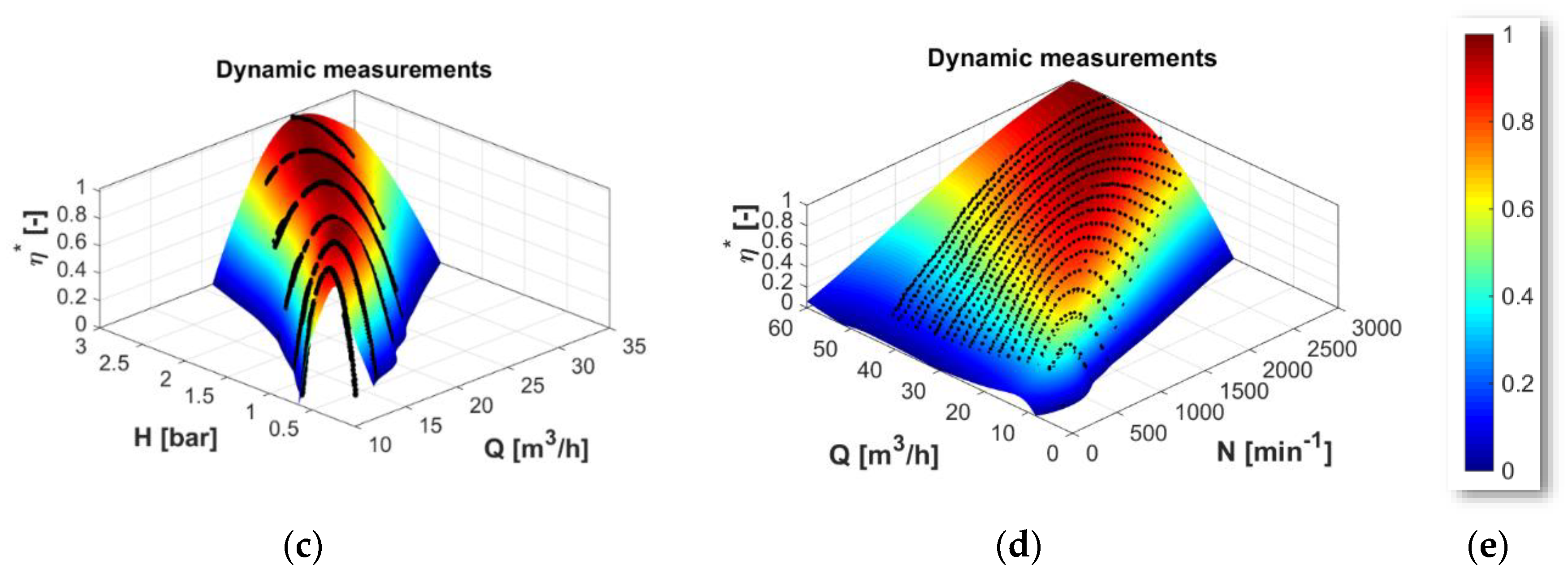
Figure 12.
Resulting efficiency 3D hill-charts obtained by classical static point-by-point and by the dynamic measurement methods: (a) counter-rotating microturbine—result of static measurements; (b) PAT—result of static measurements; (c) counter-rotating microturbine—result of dynamic measurements; (d) PAT—result of dynamic measurements; (e) colour plot scale.
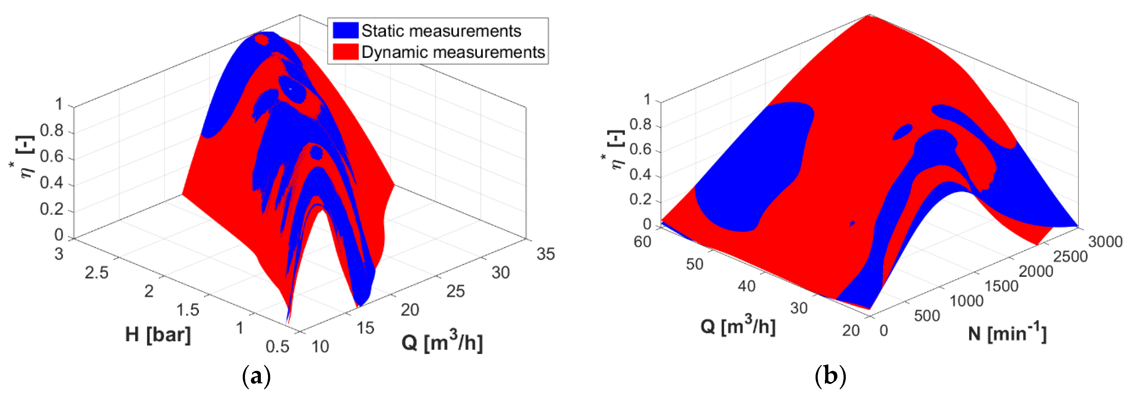
Figure 13.
Validation of resulting 3D hill-charts obtained by the dynamic measurements method with the results of the classical static point-by-point method: (a) comparison for the counter-rotating microturbine; (b) comparison for the PAT.
Figure 13.
Validation of resulting 3D hill-charts obtained by the dynamic measurements method with the results of the classical static point-by-point method: (a) comparison for the counter-rotating microturbine; (b) comparison for the PAT.
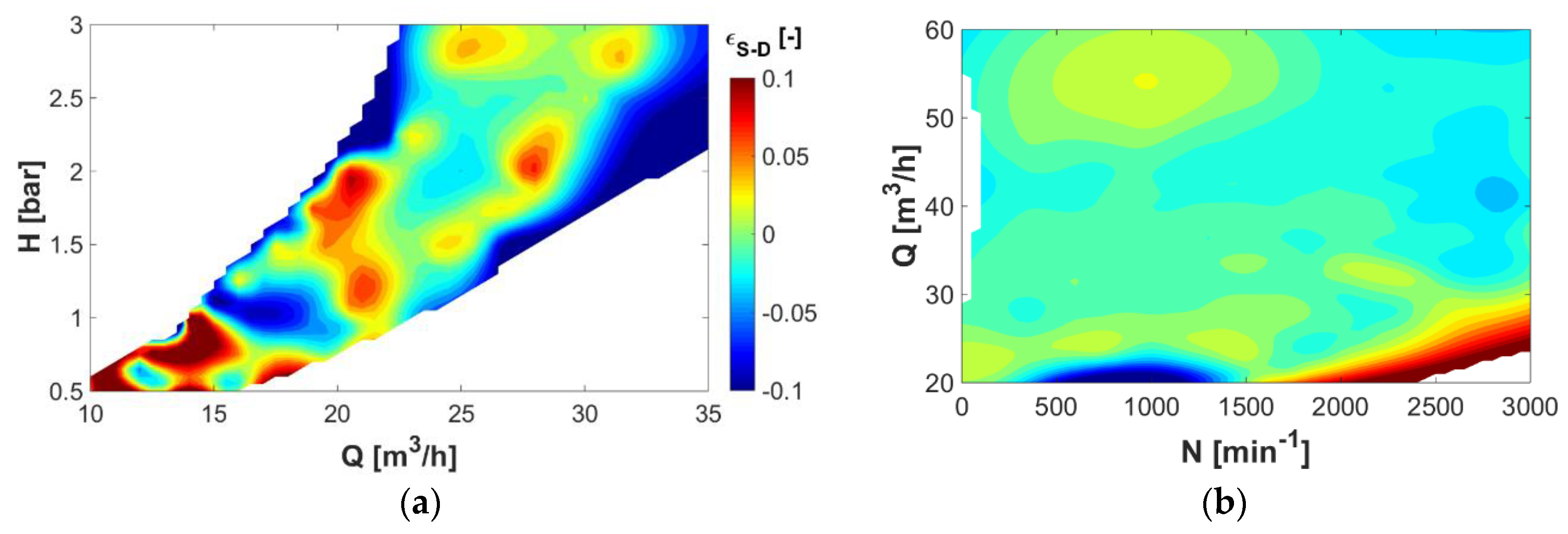
Figure 14.
Resulting contours of difference between the 3D hill-charts obtained by the dynamic measurements method compared with the results of the classical static point-by-point method: (a) result for the counter-rotating microturbine; (b) result in the case of the PAT.
Figure 14.
Resulting contours of difference between the 3D hill-charts obtained by the dynamic measurements method compared with the results of the classical static point-by-point method: (a) result for the counter-rotating microturbine; (b) result in the case of the PAT.
Table 1.
Main characteristics of the employed instruments for performance measurements.
Table 1.
Main characteristics of the employed instruments for performance measurements.
| Measured Quantity | Sensor Type | Range | Accuracy |
|---|
| Discharge (Q) | Danfoss MAGFLO MAG3100 Water electromagnetic flowmeter | 0..±100 [m3/h] | ±0.5 [%] |
| Head (H) | Endress and Hauser Deltabar M PMD55 differential pressure sensor | 0..16 [bar] | ±0.1 [%] |
| Setting level (HS) | Fuji FCX-CII Series differential pressure sensor | 0..5 [bar] | ±0.2 [%] |
| Absolute static pressure (M1,2,3,4) | Endress and Hauser Cerabar T PMC 131 capacitive pressure transducer | 0..10/20 [bar] | ±0.05 [%] |
| Water Temperature (T) | Endress and Hauser Easytemp TMR 31 PT100 transducer | 0..100 [°C] | ±0.1 [%] |
| Pumps’ rotational speed (Np1,2,3) | Sick VTF180-2P42417 photoelectric proximity sensor | 0..1000 [Hz] | - |
| Mechanical torque (Tmec A,B) | NCTE 2200 torquemeter | 0..±7.5 [Nm] | ±1 [%] |
| Turbine rotational speed (NA,B) | IED incremental encoder | 0..7500 [min−1] | 2048 [ppr] |
| Electrical power (Pelec) | Zimmer LMG500 precision electrical multimeter | 0..1000 [Vtrms]
0..32 [Atrms] | ±0.03 [%] |
| PAT rotational speed (N) | Incremental encoder | 0..6000 [min−1] | 4096 [ppr] |
| Data acquisition and control |
| NI CompactRIO 9074 controller | Dedicated to the control/monitoring of the test rig |
| NI cDAQ-9174 digitizer | Dedicated to the control/monitoring of the testing model using the standard static measurements method |
| NI cDAQ-9174 digitizer | Dedicated to the control/monitoring of the testing model for the dynamic measurements |
Table 2.
Combinations of rotational speeds of the microturbine runners for point-by-point performance measurements.
Table 2.
Combinations of rotational speeds of the microturbine runners for point-by-point performance measurements.
| H = 0.5/0.75/1/1.25/1.5/1.75/2/2.25/2.5/2.75/3 [bar] |
|---|
| NA [%] | NB [%] |
|---|
| 0 | 0 | – | – | – | – | – | – | – | – |
| 8.33 | 0 | 2.08 | 4.17 | 6.25 | 8.33 | 11.08 | 16.67 | 33.33 | 8.33 |
| 16.67 | 0 | 4.17 | 8.33 | 12.5 | 16.67 | 22.17 | 33.33 | 66.67 | 16.67 |
| 25 | 0 | 6.25 | 12.5 | 18.75 | 25 | 33.33 | 50 | 100 | 25 |
| 33.33 | 0 | 8.33 | 16.67 | 25 | 33.33 | 44.47 | 66.67 | – | 33.33 |
| 41.67 | 0 | 10.42 | 20.83 | 31.25 | 41.67 | 55.42 | 83.33 | – | 41.67 |
| 50 | 0 | 12.5 | 25 | 37.5 | 50 | 66.67 | 100 | – | 50 |
| 58.33 | 0 | 14.58 | 29.17 | 43.75 | 58.33 | 77.58 | – | – | 58.33 |
| 66.67 | 0 | 16.67 | 33.33 | 50 | 66.67 | 88.9 | – | – | 66.67 |
| 75 | 0 | 18.75 | 37.5 | 56.25 | 75 | 100 | – | – | 75 |
| 83.33 | 0 | 20.83 | 41.67 | 62.5 | 83.33 | – | – | – | 83.33 |
| 91.67 | 0 | 22.92 | 45.83 | 68.75 | 91.67 | – | – | – | 91.67 |
| 100 | 0 | 25 | 50 | 75 | 100 | – | – | – | 100 |
| α = NB/NA [−] | 0 | 0.25 | 0.5 | 0.75 | 1 | 1.33 | 2 | 4 | ∞ (NA = 0) |
Table 3.
Combinations of rotational speeds of the recirculating pumps and of the PAT for performance measurements using the static method.
Table 3.
Combinations of rotational speeds of the recirculating pumps and of the PAT for performance measurements using the static method.
| | Np1,2,3 [%] |
|---|
| 24 | 33.33 | 41.67 | 50 | 58.33 | 66.67 | 75 | 83.33 | 91.67 | 100 |
|---|
| NPAT [%] | 8.33 | 8.33 | 8.33 | 8.33 | 8.33 | 8.33 | 8.33 | 8.33 | 50 | 78 |
| 16.67 | 16.67 | 16.67 | 16.67 | 16.67 | 16.67 | 16.67 | 16.67 | 58.33 | 83.33 |
| 25 | 25 | 25 | 25 | 25 | 25 | 25 | 25 | 66.67 | – |
| 33.33 | 33.33 | 33.33 | 33.33 | 33.33 | 33.33 | 33.33 | 33.33 | 75 | – |
| 41.67 | 41.67 | 41.67 | 41.67 | 41.67 | 41.6·7 | 41.67 | 41.67 | 83.33 | – |
| 50 | – | 50 | 50 | 50 | 50 | 50 | 50 | 91.67 | – |
| 58.33 | – | 58.33 | 58.33 | 58.33 | 58.33 | 58.33 | 58.33 | 100 | – |
| – | – | – | 66.67 | 66.67 | 66.67 | 66.67 | 66.67 | – | – |
| – | – | – | 75 | 75 | 75 | 75 | 75 | – | – |
| – | – | – | – | 83.33 | 83.33 | 83.33 | 83.33 | – | – |
| – | – | – | – | 91.67 | 91.67 | 91.67 | 91.67 | – | – |
| – | – | – | – | – | 100 | 100 | 100 | – | – |
Table 4.
Microturbine runners rotational speed variation ranges for performance measurements using the dynamic method.
Table 4.
Microturbine runners rotational speed variation ranges for performance measurements using the dynamic method.
| | Np1,2,3 [%] | |
|---|
| | 24 | 33.33 | 41.67 | 50 | 58.33 | 66.67 | 75 | 83.33 | 91.67 | α = NB/NA [−] |
|---|
| NA [%] | 0 ÷ 100 | 0 ÷ 100 | 0 ÷ 100 | 0 ÷ 100 | 0 ÷ 100 | 33.33 ÷ 100 | 75 ÷ 100 | 83.33 ÷ 100 | 91.67 ÷ 100 | 0 |
| 0 ÷ 100 | 0 ÷ 100 | 0 ÷ 100 | 0 ÷ 100 | 41.67 ÷ 100 | – | – | – | – | 0.125 |
| 0 ÷ 100 | 0 ÷ 100 | 0 ÷ 100 | 0 ÷ 100 | 41.67 ÷ 100 | 83.33 ÷ 100 | – | – | – | 0.25 |
| 0 ÷ 100 | 0 ÷ 100 | 0 ÷ 100 | 0 ÷ 100 | 33.33 ÷ 100 | 58.33 ÷ 100 | 91.67 ÷ 100 | – | – | 0.5 |
| 0 ÷ 100 | 0 ÷ 100 | 0 ÷ 100 | 0 ÷ 100 | 25 ÷ 100 | 50 ÷ 100 | 75 ÷ 100 | – | – | 0.75 |
| 0 ÷ 100 | 0 ÷ 100 | 0 ÷ 100 | 0 ÷ 100 | 25 ÷ 100 | 41.67 ÷ 100 | 58.33 ÷ 100 | 83.33 ÷ 100 | – | 1 |
| 0 ÷ 75 | 0 ÷ 75 | 0 ÷ 75 | 0 ÷ 75 | 18.75 ÷ 75 | 31.25 ÷ 75 | 50 ÷ 75 | – | – | 1.33 |
| 0 ÷ 50 | 0 ÷ 50 | 0 ÷ 50 | 0 ÷ 50 | 12.5 ÷ 50 | 25 ÷ 50 | 45.83 ÷ 50 | – | – | 2 |
| 0 ÷ 25 | 0 ÷ 25 | 0 ÷ 25 | 0 ÷ 25 | 6.25 ÷ 25 | 12.5 ÷ 25 | – | – | – | 4 |
| 0 ÷ 12.5 | 0 ÷ 12.5 | 0 ÷ 12.5 | 0 ÷ 12.5 | 4.17 ÷ 12.5 | – | – | – | – | 8 |
| NB[%] | 0 ÷ 100 | 0 ÷ 100 | 0 ÷ 100 | 0 ÷ 100 | 33.33 ÷ 100 | – | – | – | – | ∞ (NA = 0) |
Table 5.
Combinations of rotational speeds of the recirculating pumps and of the PAT for performance measurements using the dynamic method.
Table 5.
Combinations of rotational speeds of the recirculating pumps and of the PAT for performance measurements using the dynamic method.
| Np1,2,3 [%] | 24 | 29.17 | 33.33 | 37.5 | 41.67 | 45.83 | 50 | 54.17 | 58.33 | 62.5 |
| 66.67 | 70.83 | 75 | 79.17 | 83.33 | 87.5 | 91.67 | 95.83 | 100 | |
| NPAT [%] | 8.33 ÷ 100 |
Table 6.
Resulting STD values of the efficiency fluctuation depending on the acceleration/deceleration ramp.
Table 6.
Resulting STD values of the efficiency fluctuation depending on the acceleration/deceleration ramp.
| Acceleration/Deceleration Ramp [s/1000 min−1] | η*’STD [%] |
|---|
| Microturbine | PAT |
|---|
| 10 | 2.6467 | 2.2774 |
| 25 | 1.1363 | - |
| 30 | - | 1.0995 |
| 40 | 0.6693 | - |
| 60 | 0.5369 | 0.7863 |
| 90 | 0.3167 | 0.6246 |
| 120 | 0.3213 | - |
Table 7.
Final balance between the two testing methods.
Table 7.
Final balance between the two testing methods.
| Criterion | Microturbine | PAT |
|---|
| Static Measurements | Dynamic Measurements | Static Measurements | Dynamic Measurements |
|---|
| Testing variable | 11× testing heads | 9× pumps’ speeds | 10× pumps’ speeds | 19× pumps’ speeds |
| Turbine runner(s) speed | 9× speed ratios, 13× runners speeds, 0 ÷ 100% speed range | 11× speed ratios, 0 ÷ 100% forth and back runners speed variation | 12× runner speeds, 8.33 ÷ 100% speed range | 0 ÷ 100% forth and back runner speed variation |
| Total measured points/curves | >1000 static operating points | ~70 dynamic curves | ~100 static operating points | 19 dynamic curves |
| Total time | ~1 men-week | ~1 men-day | ~1/2 men-day | ~1/2 men-day |


