1. Introduction
The diffraction phenomenon has been traditionally used to control beamforming and focalization of lenses in different physical fields such as optics, acoustics or microwaves. Conventional lenses’ focusing capabilities are based on their curved shapes and their refractive materials. As an alternative to traditional lenses, different solutions have been investigated such as sonic crystals [
1], planar structures built with concentric rings such as Fresnel lenses [
2] or variations on the latter, pinhole zone plates [
3]. It has been shown that these new lenses can improve focalization over traditional ones.
In the acoustic field, the modulation control of acoustic beams is an important topic, because it can result in a significant advance in different applications such as medical therapy or non-destructive material analysis, which includes a wide range of areas such as material flaw detection [
4], pest detection in agroforestry [
5] and food analysis [
6].
The use of planar structures that are capable of guiding and focusing waves the same way as traditional lenses is very interesting. Among the possible geometries that can be analyzed, fractal structures have already been proposed [
7,
8]. Particularly, Generalized Polyadic Cantor Sets (GPCSs) are very attractive because they can be generated with simple algorithms, and this is the main reason why the majority of studies are based on these type of fractals [
9,
10]. Fractal lenses have been shown to become a possible improvement on focalization properties, reducing aberration simultaneously [
11].
In this work, the design and characterization of planar acoustic lenses based on GPCSs is developed, and their application as ultrasonic lenses is analyzed. These new kinds of lenses are known as Polyadic Cantor Fractal Lenses (PCFLs). These structures are proposed because of their ease of fabrication and their multifocus profile.
2. Polyadic Cantor Fractal Lens Generation
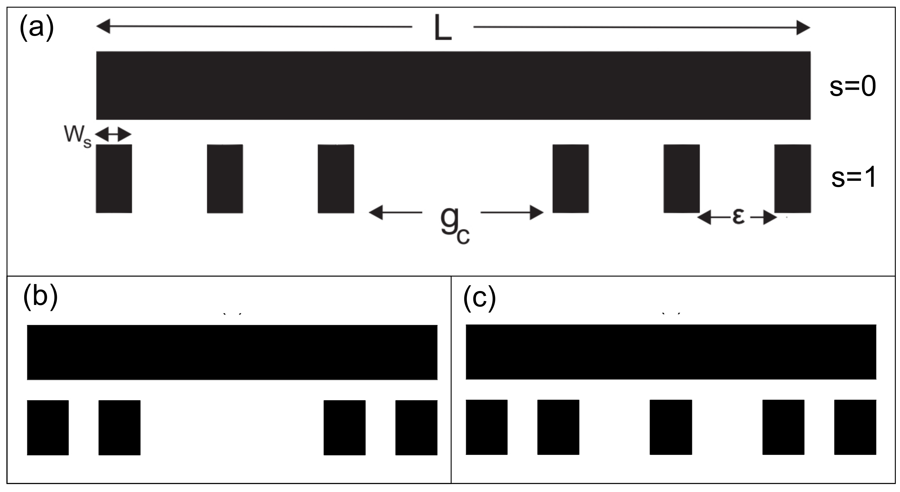
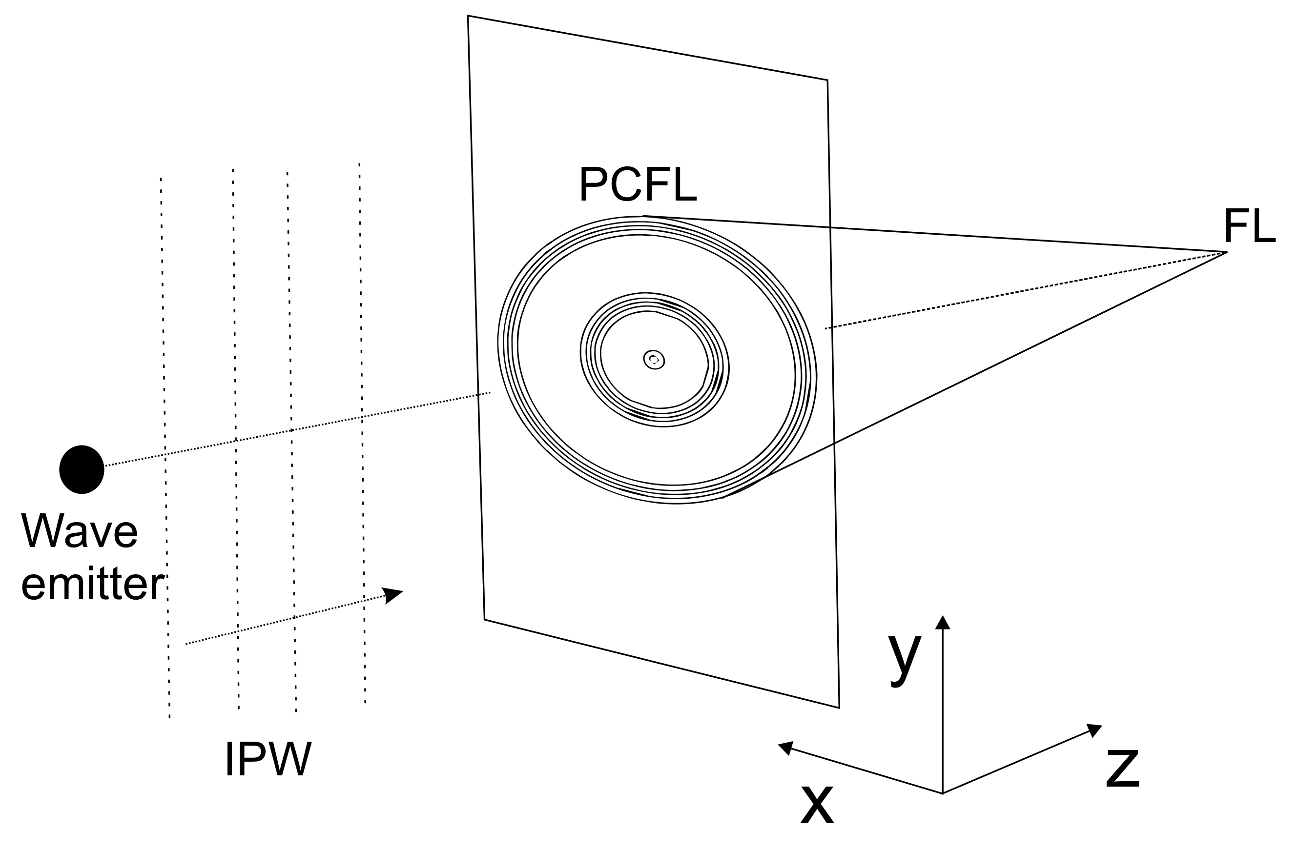
Figure 1 shows a Polyadic Cantor Fractal Lens (PCFL) across the XY-coordinate plane with plane wave excitation. The acoustic field is modulated by the lens and originates a focus on a perpendicular axis to the lens. The distance between the position of the focus and the lens plane is known as the focal distance (FL). In some applications, it may be necessary to have multiple foci.
The PCFL is built using the GPCS algorithm. First, the initial element (stage
), known as the initiator, is substituted by a set of
N segments of identical lengths
. The rparameter is known as the scaling factor and should take values from 0–1/2 in order to produce a GPCS; see
Figure 2a. These segments are separated by gaps. If
N is even, there is a central gap of width
g and
lateral gaps of width
; see
Figure 2b. If
N is odd, the central gap is split into two halves of width
g/2 at the sides of the central segment, and there are
lateral gaps of width
; see
Figure 2c. As can be seen in
Figure 2, the number of total gaps is always given by
.
This way, the stage
of the GPCS, known as the generator, is constructed. Both the initiator (
) and generator (
) have exactly the same length. This procedure is repeated as many times as required in the following stages. The number, distribution and widths of the segments of the generator affect the homogeneity and texture of the fractal. To characterize these features, parameters such as the fractal dimension (
D), the number of elements (
N), the fractal stage s, the central gap width
g and the lateral gap width
are considered; see
Figure 2a.
The fractal dimension is defined as,
with
n the total number of gaps of the generator and
r the scaling factor. If
N is fixed,
n, as well, and
r must be modified to obtain different values for the fractal dimensions. Therefore, the fractal dimension relates directly to the transparency of the fractal.
An alternative way to refer to the fractal gap distribution is through a parameter known as the central gap fraction
f. This parameter ranges from 0–1 and gives an indication of the weight of the central gap over the total gap space in the generator. The width of the central gap can be related to the central gap fraction using,
As mentioned above, the even-order GPCS has a unique central gap of width
g, while the odd-order GPCS splits the central gap into two gaps of widths
g/2 at both sides of the central segment. The lateral gap widths of the generator can be calculated with the following expressions,
As stated previously, this is a recursive procedure. In each stage, the different segments are substituted by generator copies of the same length. Thus, as the stage evolves, the number of segments increases, while the segment length decreases. At stage s, the segment lengths can be calculated with,
Although this iterative procedure can be repeated indefinitely, once the second stage () is achieved, the iterative procedure is truncated due to mechanical limitations with the construction of the device. Therefore, the final structure is not a real fractal, but a prefractal.
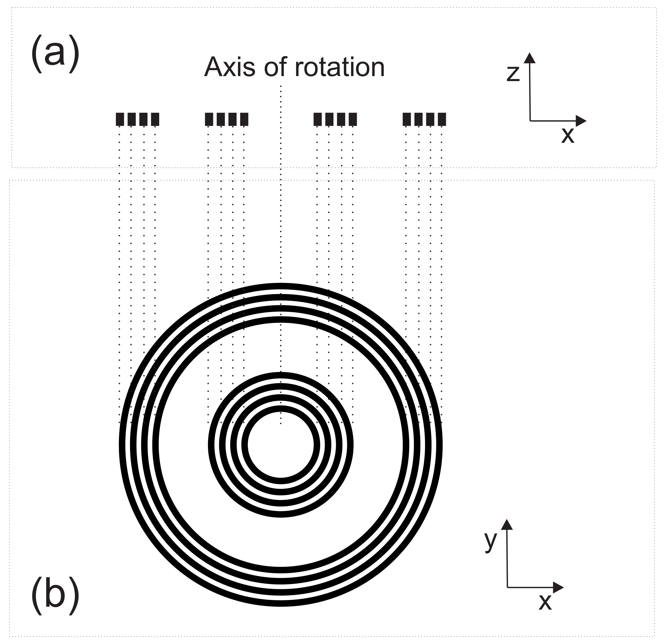
The PFCL is then generated from the prefractal structure. In order to do that, the prefractal structure revolves 180 degrees around a perpendicular axis aligned through the center of the GPCS (OZ axis); see
Figure 3a. In this way, a set of concentric rings is obtained at the OXY plane, as can be observed from
Figure 3b. The PFCL generated in the OXY plane is shown in three dimensions in
Figure 1.
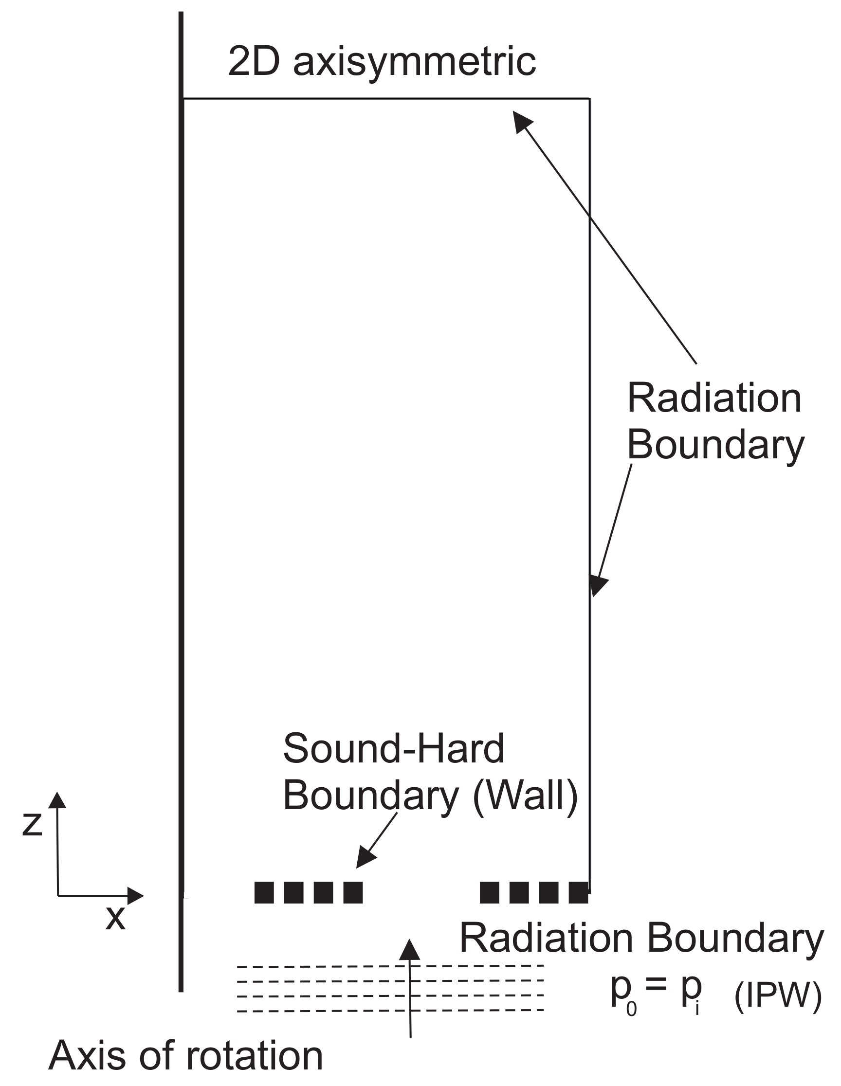
3. Numerical Model
Nowadays, there is a large number of mathematical techniques that can be used for solving acoustic problems, taking into account the interaction of ultrasonic waves with structures immersed in water. In this work, the Finite Element Method (FEM), and in particular the commercial software COMSOL Multiphysics, has been used. This software is capable of solving complex geometries with multiple acoustic phenomena. To solve the acoustic problem, it is necessary to define the geometry to be analyzed, to implement the boundary conditions correctly and to discretize the resolution domain. For this purpose, it is necessary to solve the Helmholtz equation given by,
where
(
= 1000 kg/m
) is the medium density,
c (
c = 1500 m/s) is the ultrasound velocity,
is the angular frequency and p is the acoustic pressure.
Figure 4 shows the scheme of the numerical model. It is an ideal 2D axisymmetric model, which allows 2D analysis equivalent to a more complex 3D analysis, significantly reducing the calculation loads. Computation times are reduced, because the axisymmetric model takes advantage of the revolution symmetry of the problem, which is a direct consequence of the way the PCFL has been generated as described previously. Therefore, the software solves the acoustic problem by revolving 360 degrees around a perpendicular axis aligned through the center of the GPCS (OZ axis) the 2D model and obtaining a 3D equivalent, as shown in
Figure 1.
The assumptions made in the simulations are the following: the wavelength of the incident plane wave is large compared to the thickness of the lens; the lens is considered to be acoustically rigid; therefore, the Neumann boundary condition, zero sound velocity, is applied, and finally, the plane wave radiation condition is also applied to the boundaries of the domain to simulate free space and emulate the Sommerfeld condition as shown in
Figure 4. Due to the characteristics of the system that is being modeled, where small time-dependent pressure variation values are assumed, the so-called background pressure field is considered. To quantify the acoustic field, the sound pressure level is calculated at each point in the domain, and then, the acoustic gain is calculated using the expression,
where
p is the sound pressure at an arbitrary point and
p is incident sound pressure at the lens.
4. Results and Discussion
Once the PCFL design parameters have been presented, the influence of these parameters on the modulation of the sound beam is analyzed. For this purpose, the numeric method used in the previous section was employed. The design was oriented towards the fabrication of planar acoustic lenses with focal profile control mechanisms and beamforming capabilities. A lens of radius cm and negligible thickness compared with the wavelength was designed with the following design parameters: , , . The operating frequency was set at kHz. As mentioned above, for practical reasons and the ease of construction, the prefractal stage was set at .
The results that are going to be shown correspond to sound pressure gain maps in the OXZ plane, that is the plane orthogonal to the lens that contains its center. In this plane, the location, width and intensity of the different PCFL foci can be observed. The total width of the working space was equal to 20 cm along the OX axis, whereas 80 cm have been analyzed along the OZ axis from the position of the lens forward. In the pressure maps, the lens is located just at the bottom position () of the OXZ plane.
Three different analyses have been carried out. First, the dependence of the focal distance on the operating frequency has been analyzed. Secondly, the influence of the fractal dimension on the focus location has been considered, and finally, the effect of the number of elements of the generator (N) on the focusing profile has also been studied.
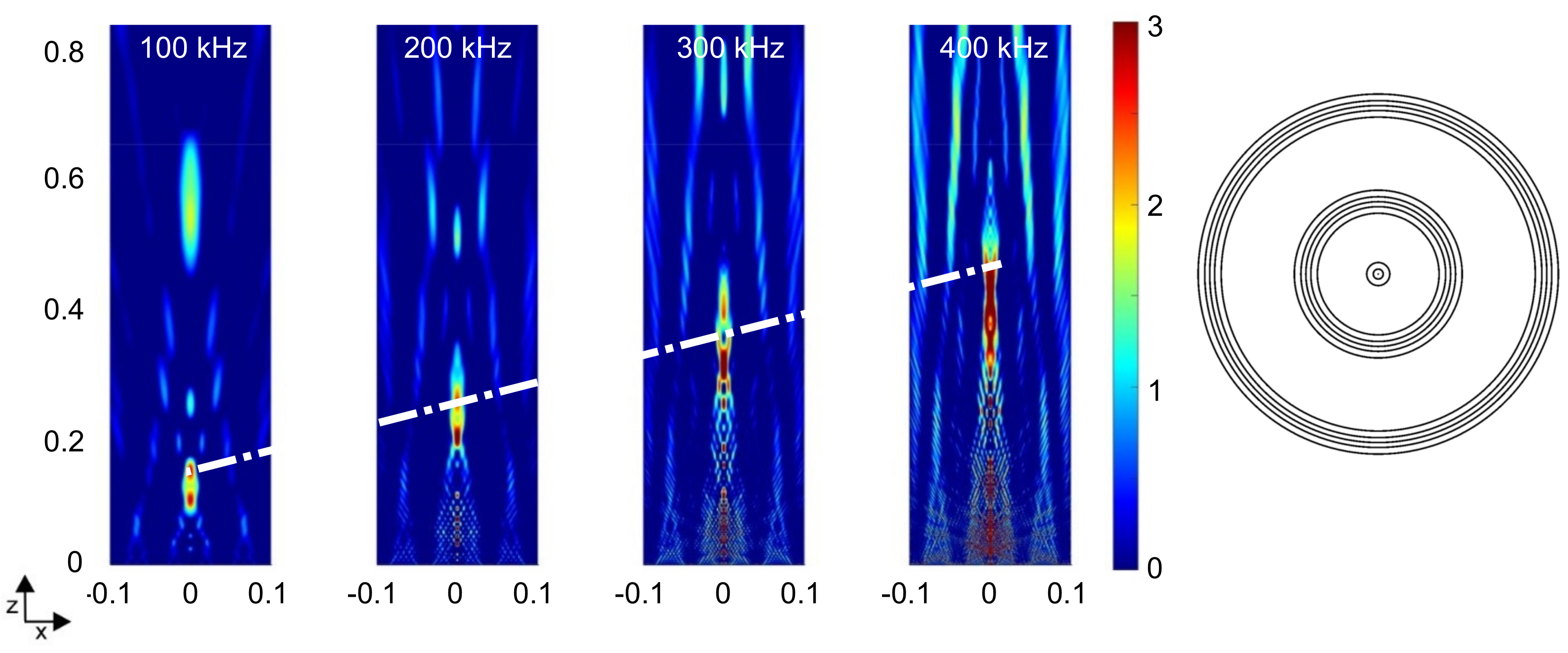
4.1. Focusing Profile Variation with Frequency
Fixing the design parameters at values
cm,
,
and
, the influence of the operating frequency variation on the PCFL focus location is analyzed.
Figure 5 shows the layout of the PCFL to be analyzed. The lens is located at the OXY plane. The sound pressure gain map is obtained at the OXZ central plane in dB units.
The operating frequency is modified from 100 kHz–400 kHz.
Figure 5 shows the simulated maps for four different frequencies. As can be observed from the figure, the location of the focus that is closer to the lens modifies its position when the operating frequency increases. This variation is linear and can be modeled with the following expression,
with
d(100 kHz) the focal distance at an operating frequency of 100 kHz and
f the operating frequency in kHz.
The graphical representation of Equation (
7) is shown with a white line on
Figure 5. It can be observed that it is a linear dependence. Once the PCFL is designed, a precise focus shifting along the Z-axis is achieved and controlled by slightly varying the operating frequency. Thus, a dynamic and effective mechanism to modify the PCFL focal length is provided.
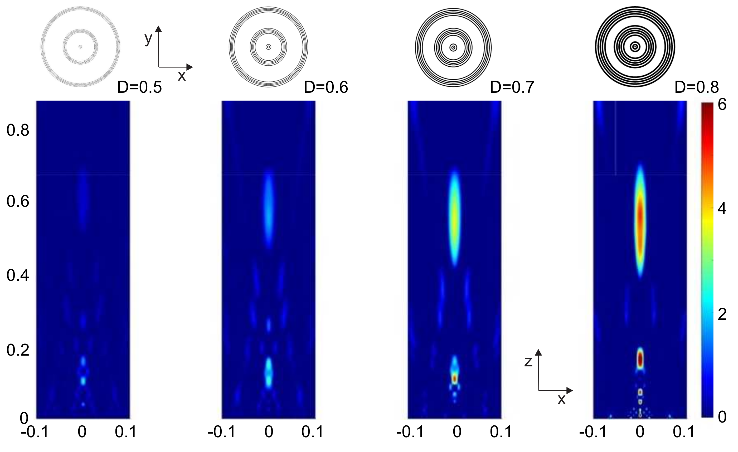
4.2. Focusing Profile Variation with Fractal Dimension
Fixing the design parameters at values
cm,
kHz,
and
, the influence of the fractal dimension variation on the PCFL focusing profile is analyzed. Thus, fractal dimension has been modified between 0.5 and 0.8, with the results are shown in
Figure 6. As can be observed, the foci location does not change. However, a significant increase of the sound intensity can be observed when the fractal dimension becomes higher.
From the figure, it can also be observed that the lens becomes less transparent when the fractal dimension increases. It can be concluded that the fractal dimension affects the gain of the main focus on the pressure map.
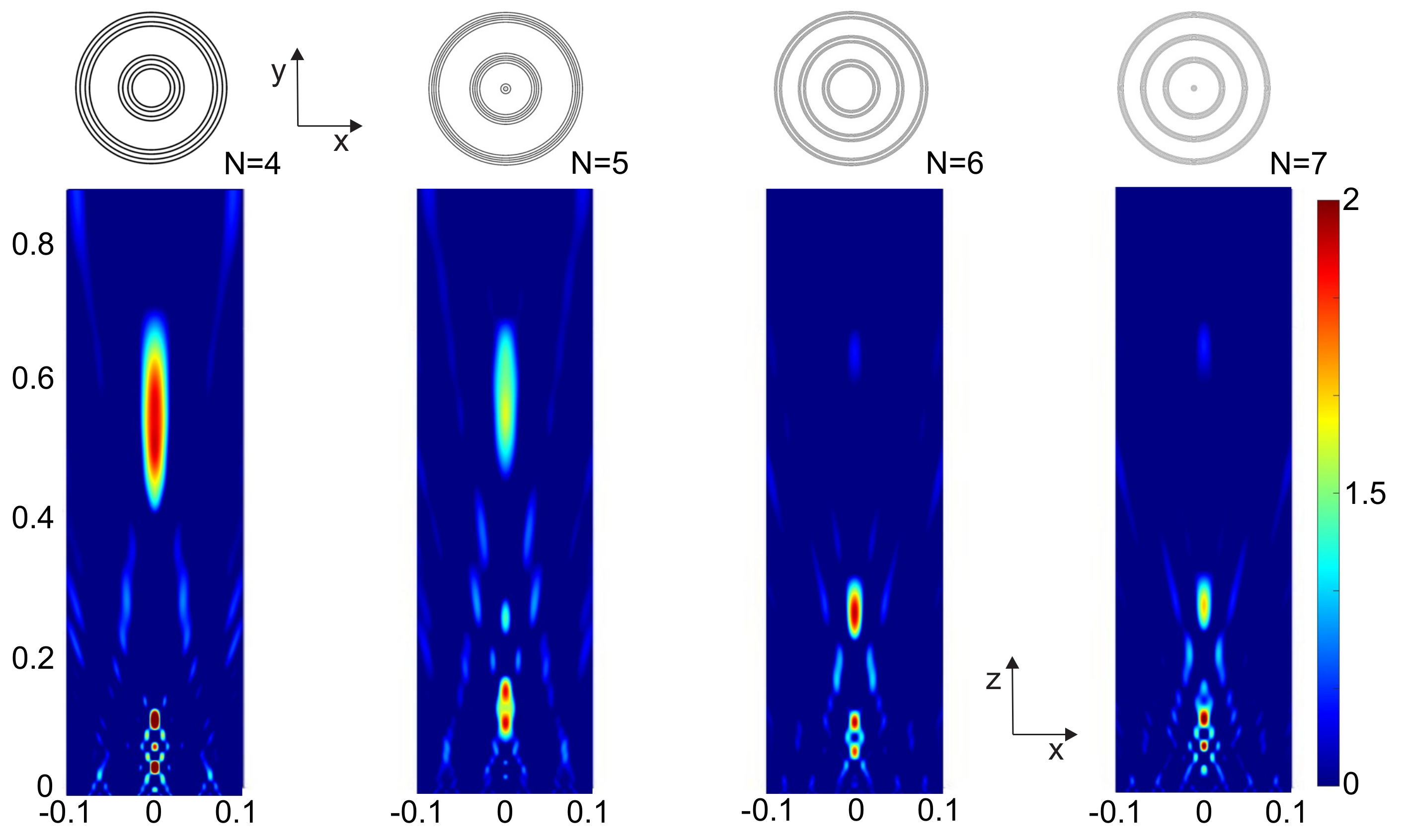
4.3. Focusing Profile Variation with the Number of Elements
Fixing the design parameters at values cm, kHz, and , the influence of the number of elements of the generator on the PCFL beamforming capabilities is analyzed. This parameter has been modified between and .
Table 1 shows the dependence of parameters r and
g with
N. Increasing
N results in a decrease in r if the fractal dimension is kept constant, as a result of the elements becoming smaller. However, this inverse relationship is not linear, as can be observed in Equation (
1) Therefore, the opacity percentage of the PCFL diminishes when
N is increased, and the central gap becomes higher. Thus, increasing the number of elements
N makes the lens slightly more transparent without requiring the variation of the fractal dimension; see
Figure 7.
As can be observed from
Figure 7, varying the number of elements (
N) at Stage 1 (
) allows one to enhance the gain of further or closer foci.

 ,
, 
