A Trajectory Planning Method for Polishing Optical Elements Based on a Non-Uniform Rational B-Spline Curve

Abstract

Optical polishing can accurately correct the surface error through controlling the dwell time of the polishing tool on the element surface. Thus, the precision of the trajectory and the dwell time (the runtime of the trajectory) are important factors affecting the polishing quality. This study introduces a systematic interpolation method for optical polishing using a non-uniform rational B-spline (NURBS). A numerical method for solving all the control points of NURBS was proposed with the help of a successive over relaxation (SOR) iterative theory, to overcome the problem of large computation. Then, an optimisation algorithm was applied to smooth the NURBS by taking the shear jerk as the evaluation index. Finally, a trajectory interpolation scheme was investigated for guaranteeing the precision of the trajectory runtime. The experiments on a prototype showed that, compared to the linear interpolation method, there was an order of magnitude improvement in interpolation, and runtime, errors. Correspondingly, the convergence rate of the surface error of elements improved from 37.59% to 44.44%.

1. Introduction

With the rapid development of astronomy, space exploration, and advanced optical instruments, optical elements are being increasingly widely used. The application demands for high-quality and high-efficiency elements present distinct higher requirements for the process technology used in such elements [1]. Computer-controlled optical surfacing (CCOS) has been successfully applied in industrial production, as it can precisely correct the surface error by converting the dwell time of the polishing tool into the feed-rate along the polishing trajectory. Therefore, a trajectory planning method is the key factor affecting high-quality, high-efficiency polishing.

Despite the extent of research on path planning in some fields [2,3,4], investigation of optical polishing has been rather limited. Although the problem of discontinuous surfaces between the adjacent mm-sized short line segments has attracted wide concern when using parametric curve theory [5,6,7], frequent acceleration and deceleration result in poor realisation precision of dwell time, i.e., the runtime of trajectory (hereafter referred to as runtime), which further influences the polishing quality of elements and the convergence rate of surfaces [8]. The main focus of this paper is to investigate an interpolation scheme to overcome the above problem, which has two main progressive aspects: fitting and interpolation of parametric curves.

The fitting of parametric curves is a process of converting discrete short line segments into parametric curves. At present, many scholars have carried out research based on the dominant points using a non-uniform rational B-spline (NURBS). Park [9,10] proposed a method for determining the dominant points according to the discrete curvature. Zhou [11] and Xu [12] improved this method by taking concave-convex turning points and extreme points on the curvature curve as dominant points. To improve the fitting precision, Zhao [13] proposed curve fitting taking squared distance minimisation (SDM) as the evaluation index. Although the dominant points based method is easy with regard to calculation and interpolation, it may result in the loss of runtime at non-dominant points. Thus, only the global fitting method is suitable to the optical polishing. To do so, Yang [14] proposed an optimisation algorithm by establishing the evaluation function for deviation of the fitted distance. Li [15] and Lin [16] classified the trajectory into the different forms of NURBS and then employed a piecewise fitting method for real-time implementation. Based on Gaussian elimination and the continuous short block (CSB) look-ahead algorithm, Tsai [17] and Wang [18] realised the on-line transformation from short line segments to NURBS: however, for the global fitting method, the simplified strategy that setting all the weight factors as 1 eliminates the regulating effect on the fairness of curves and easily causes curvature saltation on the trajectory. Therefore, generating a fair trajectory based on NURBS is the first problem facing the polishing trajectory planning technique.

The interpolation of parametric curves is a process that discretises the NURBS into numerical control (NC) commands. Speed planning, as the critical step in the interpolation process, has been an area of research for numerous scholars: this can be classified into the time-optimal approach and the non-time-optimal approach. The time-optimal approach deals with the planning problem by taking the minimisation of the motion time as the objective to promote manufacturing efficiency [19,20]. For example, Timar [21] proposed a speed planning scheme for NC interpolation by the use of the optimal control theory. On this basis, Sencer [22] and Lu [23] considered the driving capacity constraint and trajectory precision constraint in the interpolation, respectively. The non-time-optimal approach usually deals with the planning problem by taking the minimisation of speed fluctuations as the objective [24]. Various methods, such as the feed-rate evolutionary algorithm [25], the equidistance quaternion method [26], and the improved Adams-Malton algorithm [27] are employed to decrease speed fluctuations and guarantee steady, continuous-trajectory operation. Although the effectiveness of the method has been validated experimentally, is cannot be applied directly to optical polishing because the effect of acceleration and deceleration on the realisation precision of runtime is not considered.

Driven by the practical needs to improve the quality of optical polishing, this paper presents a systematic trajectory planning method that particularly enhances the realisation precision of runtime. Following this introduction, Section 2 calculates all the control points of NURBS through numerical solution to overcome the problem of calculation efficiency. In Section 3, an optimisation algorithm of fairing NURBS is established by taking the shear jerk of trajectory as an evaluation index. Section 4 then proposes an interpolation scheme with which to minimise the realisation error of runtime by planning the feed-rate of trajectory according to the given runtime between adjacent NC codes. Section 5 reports experiments on a prototype machine which shows that the proposed trajectory planning method is more accurate than the linear interpolation method. Conclusions are drawn in Section 6.

2. Trajectory Fitting Based on the NURBS Curve

In this section, according to the given NC codes, all the control points of NURBS are solved, which provides the necessary mathematical model for the interpolation of parametric curves. The basic settings are as follows:

(1) Considering the stability, ease of use and calculation efficiency, cubic NURBS is employed as the fitting tool. (2) The uniform parametric method is used for trajectory fitting, because the polishing elements have a large radius of curvature and the chord lengths between NC codes are distributed uniformly. (3) All weight factors are set to 1. In this case, the NURBS can be treated as a cubic B-spline to simplify the calculation process.

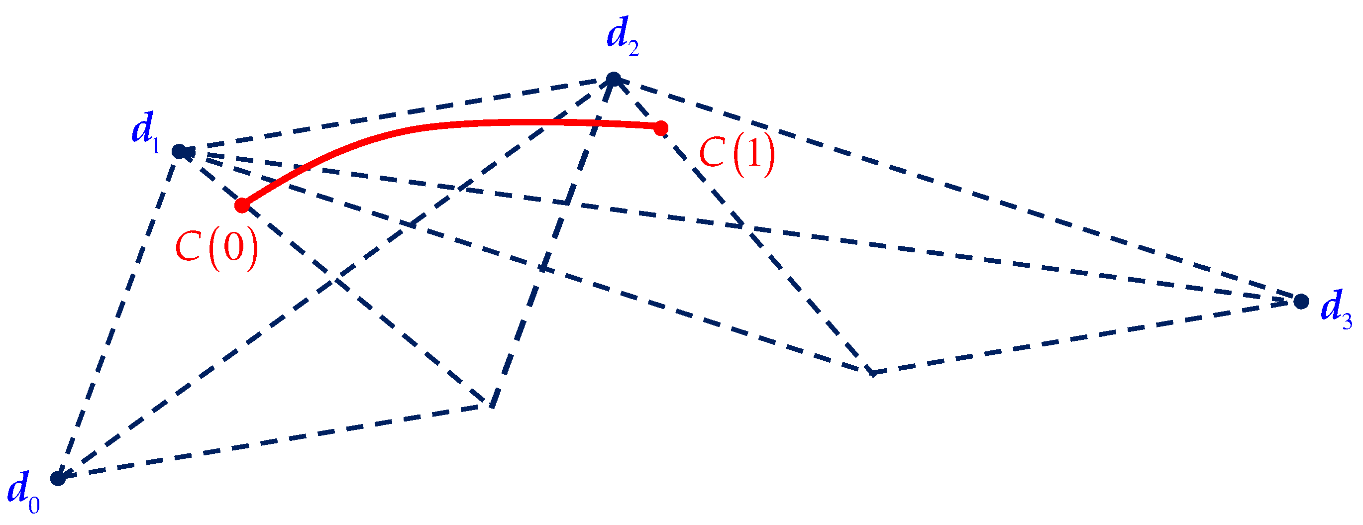
According to the basic theory of the NURBS, a segment of NURBS $C\left(u\right)\left(0\le u\le 1\right)$ can be determined based on the four adjacent control points $d_k\left(k=0,1,2,3\right)$. As shown in Figure 1, $C\left(0\right)$ and $C\left(1\right)$ separately refer to the start point and the end point of the NURBS segment. Based on the aforementioned setting, the NURBS segment can be directly written as:

$$C\left(u\right)=\frac{1}{6}\left[\begin{array}{cccc}{u}^3& u^2& u& 1\end{array}\right]\left[\begin{array}{cccc}-1& 3& -3& 1\\ 3& -6& 3& 0\\ -3& 0& 3& 0\\ 1& 4& 1& 0\end{array}\right]\left[\begin{array}{c}{d}_0\\ d_1\\ d_2\\ d_3\end{array}\right]$$

(1)

Thus, point $C_i$ can be expressed as:

$$C_i=\frac{1}{6}\left(d_{i-1}+4d_i+d_{i+1}\right)$$

(2)

where $C_i$ denotes the ith NC code in the $n+1$ lines of NC codes and also is taken as the start point of the ith NURBS segment. $d_{i-1},d_i,d_{i+1}$ respectively denote the three control points corresponding to $C_i$. To calculate $C_1$ and $C_{n+1}$, it is defined that on the condition that $i<1$, then $d_i=d_1$ and on the condition that $i>n+1$, then $d_i=d_{n+1}$. Equations (3) and (4) can thus be obtained:

$$C_1=\frac{1}{6}\left(d_1+4d_1+d_2\right)=\frac{5}{6}{d}_1+\frac{1}{6}{d}_2$$

(3)

$$C_{n+1}=\frac{1}{6}\left(d_n+4d_{n+1}+d_{n+1}\right)=\frac{1}{6}{d}_n+\frac{5}{6}{d}_{n+1}$$

(4)

Rewriting Equations (2)–(4) in matrix notation yields:

$$\begin{gathered} Ad=C \\ A=\left[\begin{array}{ccccccc}5& 1& 0& 0& 0& \dots & 0\\ 1& 4& 1& 0& 0& \dots & 0\\ 0& 1& 4& 1& 0& \dots & 0\\ ⋮& ⋮& ⋮& ⋮& ⋮& \dots & ⋮\\ 0& 0& 0& 0& 1& 4& 1\\ 0& 0& 0& 0& 0& 1& 5\end{array}\right],d=\left[\begin{array}{c}{d}_1\\ d_2\\ d_3\\ ⋮\\ d_n\\ d_{n+1}\end{array}\right],C=\left[\begin{array}{c}6C_1\\ 6C_2\\ 6C_3\\ ⋮\\ 6C_n\\ 6C_{n+1}\end{array}\right] \end{gathered}$$

(5)

If the traditional solution methods such as Gauss elimination method and LU decomposition are directly applied to the Equation (5), it may lead to some undesirable phenomena (such as excessive calculation time) due to the large quantity of NC codes for polishing. Hence, the SOR iterative algorithm [28] is used to find stable numerical solutions of Equation (5) as described below.

The coefficient matrix $A$ can be divided into:

$$A=D-L-U$$

(6)

where $A=\mathrm{diag}\left(a_{11},a_{22},\dots ,a_{n+1n+1}\right)$, $-L$ denotes a strictly lower triangular matrix, whose elements below the principal diagonal are corresponding elements of $A$. $-U$ denotes a strictly upper triangular matrix, whose elements above the principal diagonal are corresponding elements of $A$. Owing to the matrix $D$ being invertible, Equation (5) can be modified to:

$$d=D^{-1}\left(L+U\right)d+D^{-1}C$$

(7)

In this case, corner marks $\left(k\right)$ and $\left(k+1\right)$ are added in Equation (7) to identify the number of iterations. Then, the elementary iterative scheme of $d$ can be written as:

$$d^{\left(k+1\right)}=M_1{d}^{\left(k\right)}+D^{-1}C$$

(8)

where $M_1=D^{-1}\left(L+U\right)$. The component form of Equation (8) can be expressed as:

$$d_i^{\left(k+1\right)}=\frac{1}{a_{ii}}\left(-{\displaystyle \sum _{\begin{array}{l}j=1\\ j\ne i\end{array}}^{n+1}{a}_{ij}{d}_j^{\left(k\right)}+C_i}\right),i=1,2,\dots ,n+1$$

(9)

which is also known as the Jacobi iteration scheme, noting that, before calculating $d_i^{\left(k+1\right)}$, the iterative values of the first $i-1$ components in $d^{\left(k+1\right)}$ have been generated, which are more approximate to the true value than the results obtained by the previous iteration. Therefore, $d_1^{\left(k\right)},d_2^{\left(k\right)},\dots ,d_{i-1}^{\left(k\right)}$ can be replaced by $d_1^{\left(k+1\right)},d_2^{\left(k+1\right)},\dots ,d_{i-1}^{\left(k+1\right)}$ to make $d_i^{\left(k+1\right)}$ closer to the true value. To improve the convergence rate of the iteration further, a proper parameter $\mu$ is selected to conduct the weighted averaging on the aforementioned iterative scheme:

$$d_i^{\left(k+1\right)}=\mu {\tilde{d}}_i^{\left(k+1\right)}+\left(1-\mu \right)d_i^{\left(k\right)},i=1,2,\dots n+1$$

(10)

with:

$${\tilde{d}}_i^{\left(k+1\right)}=\frac{1}{a_{ii}}\left(-{\displaystyle \sum _{j=1}^{i-1}{a}_{ij}{d}_j^{\left(k+1\right)}-{\displaystyle \sum _{j=i+1}^{n+1}{a}_{ij}{d}_j^{\left(k\right)}+C_i}}\right)$$

(11)

Substituting Equation (11) into Equation (10) leads to the SOR iteration scheme:

$$a_{ii}{d}_i^{\left(k+1\right)}+\mu {\displaystyle \sum _{j=1}^{i-1}{a}_{ij}{d}_j^{\left(k+1\right)}=a_{ii}{d}_i^{\left(k\right)}-\mu {\displaystyle \sum _{j=i}^{n+1}{a}_{ij}{d}_j^{\left(k\right)}}}+\mu C_i\hspace{0.17em},\hspace{0.17em}i=1,2,\dots ,n+1$$

(12)

Note that $A$ is a tridiagonal positive definite matrix, so the optimal value ${\mu }_{opt}$ of the relaxation factor can be expressed as [29]:

$${\mu }_{opt}=\frac{2}{1+\sqrt{1-{\left[\rho \left(M_1\right)\right]}^2}}$$

(13)

where $\rho \left(M_1\right)$ denotes the spectral radius of $M_1$.

It is worth noting that, for a flat element, the aforementioned method can be directly applied to calculate the NURBS trajectory, but for a curved element, the polishing shaft should always lie along the normal direction of the element. In this case, it is necessary to solve two trajectories of end-point and reference-point on the polishing shaft to determine the polishing attitude (for more details, please see [21]).

3. Fairing of the NURBS

Although the constructed cubic NURBS by the above method satisfies the G2 continuity characteristics, i.e., the second-order derivative functions of the trajectory is continuous, the motion stability of the trajectory is still influenced by curvature saltation. In this section, a fairing optimisation method is proposed by adjusting the weight factors of NURBS.

The fairing optimisation can be classified into two categories, i.e., global and local fairing according to the number of the adjusted point on NURBS. Considering the significant computational burden of global fairing caused by the large quantity of NC codes for polishing, it is more reasonable to modify the outlier points with curvature saltation by the use of local fairing, which are selected from all NC codes [30]. A filtering process is needed to eliminate the influence of curvature fluctuations caused by discrete calculation.

In the fairing optimisation, the shear jerk of the outlier point is taken as the evaluation index:

$$D_j=\frac{{\kappa }_{next1}-{\kappa }_j}{\Vert C_{next1}-C_j\Vert }-\frac{{\kappa }_j-{\kappa }_{last1}}{\Vert C_j-C_{last1}\Vert }$$

(14)

where ${\kappa }_j$ denotes the curvature at the jth outlier point $C_j$, ${\kappa }_{next1}$ and ${\kappa }_{last1}$ denote the curvature of the $C_{next1}$ and $C_{last1}$, which are on two adjacent sides of the outlier point. The index indicates the curvature changes of the adjacent outlier points.

To generate the weight factors of the various outlier points, the objective function is defined as:

$$L={\displaystyle \sum _{j=1}^k{D}_j^2+{\left(C_j-C_{j,0}\right)}^2}$$

(15)

where $C_{j,0}$ denotes the jth outlier point before optimisation. It can be seen from Equation (15) that the objective function is composed of two parts: part one is the curvature changes of the outlier point after optimisation, and part two is the adjustment amplitude of outlier points before, and after, optimisation. Thus, the objective function means that fairing optimisation is performed on the premise of modifying the NURBS as little as possible.

According to affine invariant principle of NURBS [31], the four-dimensional (4D) space constructed by the control points and weight factors can be expressed as:

$$C^{\omega }\left(u\right)={\displaystyle \sum _{i=1}^{n+1}{N}_{i,3}\left(u\right)\left[\begin{array}{c}{\omega }_i{d}_i\\ {\omega }_i\end{array}\right]}={\displaystyle \sum _{i=1}^{n+1}{N}_{i,3}\left(u\right)d_i^{\omega }}$$

(16)

Then, the NURBS defined by Equation (1) can be regarded as the projection of the curve $C^{\omega }\left(u\right)$ in 4D space on the centre of the hyperplane $\omega =1$. Based on Equation (2), it can be seen that:

$$C_j^{\omega }=\frac{1}{6}{d}_{j,last1}^{\omega }+\frac{2}{3}{d}_j^{\omega }+\frac{1}{6}{d}_{j,next1}^{\omega }$$

(17)

$$C_{j,last1}^{\omega }=\frac{1}{6}{d}_{j,last2}^{\omega }+\frac{2}{3}{d}_{j,last1}^{\omega }+\frac{1}{6}{d}_j^{\omega }$$

(18)

$$C_{j,next1}^{\omega }=\frac{1}{6}{d}_j^{\omega }+\frac{2}{3}{d}_{next1}^{\omega }+\frac{1}{6}{d}_{next2}^{\omega }$$

(19)

where $d_j^{\omega }$ denotes the control point corresponding to the jth outlier point and $d_{next1}^{\omega },d_{next2}^{\omega }$ and $d_{last1}^{\omega },d_{last2}^{\omega }$ denote the control points on the two adjacent sides of the control point $d_j^{\omega }$, respectively.

Furthermore, Equation (15) can be written in 4D space as:

$$L^{\omega }={\displaystyle \sum _{j=1}^k{\left(D_j^{\omega }\right)}^2+{\left(C_j^{\omega }-C_{j,0}^{\omega }\right)}^2}$$

(20)

where $C_j^{\omega }-C_{j,0}^{\omega }$ can be equivalently simplified as $d_j^{\omega }-d_{j,0}^{\omega }$ and $D_j^{\omega }$ can be approximately expressed as [32]:

$$D_j^{\omega }\approx \frac{{\left(C_{j,next1}^{\omega }\right)}^{\prime \text{}\prime }-{\left(C_j^{\omega }\right)}^{\prime \text{}\prime }}{l_{j,next1}^{\omega }}-\frac{{\left(C_j^{\omega }\right)}^{\prime \text{}\prime }-{\left(C_{j,last1}^{\omega }\right)}^{\prime \text{}\prime }}{l_{j,last1}^{\omega }}$$

(21)

where ${\left(C_j^{\omega }\right)}^{\prime \text{}\prime }$ denotes the second derivative of the NURBS at $C_j^{\omega }$, $l_{j,next1}^{\omega }=\Vert C_{j,next1,0}^{\omega }-C_{j,0}^{\omega }\Vert$ and $l_{j,last1}^{\omega }=\Vert C_{j,0}^{\omega }-C_{j,last1,0}^{\omega }\Vert$. Substituting Equation (21) into Equation (20) yields:

$$L^{\omega }={\displaystyle \sum _{j=1}^k\left(\frac{{\left(C_{j,next1}^{\omega }\right)}^{\prime \text{}\prime }-{\left(C_j^{\omega }\right)}^{\prime \text{}\prime }}{l_{j,next1}^{\omega }}-\frac{{\left(C_j^{\omega }\right)}^{\prime \text{}\prime }-{\left(C_{j,last1}^{\omega }\right)}^{\prime \text{}\prime }}{l_{j,last1}^{\omega }}\right)+{\left(d_j^{\omega }-d_{j,0}^{\omega }\right)}^2}$$

(22)

To calculate the minimum value of $L^{\omega }$, the partial derivative of Equation (22) about $d_j^{\omega }$ is set to 0:

$$\begin{array}{l}\frac{\partial L^{\omega }}{\partial d_j^{\omega }}={\displaystyle \sum _{j=1}^{k}2\left(\frac{d_{j,next2}^{\omega }-3d_{j,next1}^{\omega }+3d_j^{\omega }-d_{j,last1}^{\omega }}{l_{j,next1}^{\omega }}-\frac{d_{j,next1}^{\omega }-3d_j^{\omega }+3d_{j,last1}^{\omega }-d_{j,last2}^{\omega }}{l_{j,last1}^{\omega }}\right)}\\ \hspace{0.17em}\hspace{0.17em}\hspace{0.17em}\hspace{0.17em}\hspace{0.17em}\hspace{0.17em}\hspace{0.17em}\hspace{0.17em}\hspace{0.17em}\hspace{0.17em}\hspace{0.17em}\hspace{0.17em}\hspace{0.17em}\hspace{0.17em}\hspace{0.17em}\hspace{0.17em}\hspace{0.17em}\hspace{0.17em}\hspace{0.17em}\hspace{0.17em}·\left(\frac{3}{l_{j,next1}^{\omega }}+\frac{3}{l_{j,last1}^{\omega }}\right)+2\left(d_j^{\omega }-d_{j,0}^{\omega }\right)=0\end{array}$$

(23)

Then, the equations for $d_1^{\omega },d_2^{\omega },\dots ,d_k^{\omega }$ can be expressed as:

$$\begin{gathered} A^{\omega }{d}^{\omega }=C^{\omega } \\ {A}^{\omega }=diag\left({\left(\frac{3}{l_{j,next1}^{\omega }}+\frac{3}{l_{j,last1}^{\omega }}\right)}^2+1\right) \\ {d}^{\omega }={\left(d_1^{\omega },d_2^{\omega },\dots ,d_k^{\omega }\right)}^{\mathrm{T}} \\ {C}^{\omega }={\left(C_1^{\omega },C_2^{\omega },\dots ,C_k^{\omega }\right)}^{\mathrm{T}} \\ {C}_j^{\omega }=d_{j,0}^{\omega }-\left(\frac{d_{j,next2}^{\omega }-3d_{j,next1}^{\omega }-d_{j,last1}^{\omega }}{l_{j,next1}^{\omega }}-\frac{d_{j,next1}^{\omega }+3d_{j,last1}^{\omega }-d_{j,last2}^{\omega }}{l_{j,last1}^{\omega }}\right)\left(\frac{3}{l_{j,next1}^{\omega }}+\frac{3}{l_{j,last1}^{\omega }}\right) \end{gathered}$$

(24)

According to Equation (24), the optimised control points and weight factors corresponding to the outlier points can then be generated.

4. NURBS Interpolation

The NURBS interpolation is used to discretise the parametric curve to the NC commands based on the planned feed-rate. In this section, an interpolation method for optical polishing is proposed aiming to minimise the realisation error of the trajectory runtime.

4.1. Feed-Rate Planning

Feed-rate planning is the main influencing factor in interpolating the NC commands along the trajectory. For the optical polishing, to guarantee the desired runtime of trajectory, the specific method is displayed as follows:

Step 1: considering that now there is no analytical solution to calculate the length of NURBS, the Simpson formula is used to obtain the estimation of the length through numerical iteration:

$$p=\frac{up-low}{6}\left(f\left(low\right)+4f\left(mid\right)+f\left(up\right)\right)$$

(25)

with:

$$f\left(u\right)=\frac{ds}{du}=\sqrt{x^{\prime }\left(u\right)+y^{\prime }\left(u\right)+z^{\prime }\left(u\right)}$$

(26)

where $x^{\prime }\left(u\right),y^{\prime }\left(u\right),z^{\prime }\left(u\right)$ respectively denote the first-order derivatives of $x\left(u\right),y\left(u\right),z\left(u\right)$, which are the one-dimensional curves of $C\left(u\right)$ along $x,y,z$ axes. $up$ and $low$ denote the upper and lower boundaries of $u$, $mid=\left(up+low\right)/2$.

Step 2: the length between the two points corresponding to the parameters $up$ and $low$ is calculated:

$$l=\Vert C\left(up\right)-C\left(low\right)\Vert$$

(27)

Step 3: the error between the aforementioned two lengths is calculated:

$$e=\left|p-l\right|$$

(28)

The convergence threshold $\left[e\right]$ is given. If $e>\left[e\right]$, let $up=mid$ and repeat Steps 1 and 2. If $e<\left[e\right]$, turn to Step 4.

Step 4: the parameter interval $\left(0,1\right)$ was sectioned by the equivalent distance $up-low$ to generate the knot vector $\left(u_0,u_1,\dots ,u_n\right)$. Thus, the length of the NURBS is:

$$s\approx {\displaystyle \sum _{i=1}^n\Vert C\left(u_i\right)-C\left(u_{i-1}\right)\Vert }$$

(29)

Equipped with the length at hand, the S-curve motion law is invoked to guarantee that the feed-rates of the adjacent NURBS segments are changed smoothly. Moreover, the initial sections of the trajectory segments are defined as the feed-rate transition zone. Then, the feed-rates remain constant until the end of the trajectory segments. In this case [33]:

$$s=2v_{low}{t}_a+J{t}_a^3+v_{up}{t}_v$$

(30)

$$v_{up}=v_{low}+J{t}_a^2$$

(31)

where $v_{low}$ and $v_{up}$ denote the initial and final feed-rates of the trajectory segment. $J$, $2t_a$ and $t_v$ denote the jerk, acceleration (deceleration) time and the uniform motion time, respectively. Thus, the runtime of the trajectory segment is $t_d=2t_a+t_v$.

It is worth noting that previous studies have shown that the feed-rates, when limited by the runtime of the trajectory segments, are much lower than the maximum value which is constrained by the chord error and the driving capacity. Therefore, there is no need to check the feed-rate again.

4.2. NURBS Interpolation

The essence of interpolation is to generate the NC command along the trajectory according to the period $t_s$. As each interpolation point of the NURBS corresponds to one curve parameter, only the curve parameters need to be solved.

Taking $u$ as the function of $t$, the second-order Taylor expansion can be expressed as:

$$u_{i+1}=u_i+{\frac{du}{dt}|}_{t=t_i}{t}_s+\frac{1}{2}{\frac{d^{2}u}{d{t}^2}|}_{t=t_i}{t}_s^2$$

(32)

The feed-rate $v\left(u\right)$ can be written as:

$$v\left(u\right)=\Vert \frac{dC\left(u\right)}{du}\Vert =\Vert \frac{dC\left(u\right)}{du}\frac{du}{dt}\Vert$$

(33)

Furthermore:

$$\frac{du}{dt}=\frac{v\left(u\right)}{\Vert C^{\prime }\left(u\right)\Vert }$$

(34)

Calculating the derivative of Equation (34):

$$\frac{d^{2}u}{d{t}^2}=\frac{\frac{dv\left(u\right)}{du}\frac{du}{dt}}{\Vert C^{\prime }\left(u\right)\Vert }-v\left(u\right)\frac{\frac{d\left(\Vert C^{\prime }\left(u\right)\Vert \right)}{du}\frac{du}{dt}}{{\Vert C^{\prime }\left(u\right)\Vert }^2}$$

(35)

where:

$$\frac{d\left(\Vert C^{\prime }\left(u\right)\Vert \right)}{du}=\frac{C^{″}\left(u\right)\cdot C^{\prime }\left(u\right)}{\Vert C^{\prime }\left(u\right)\Vert }$$

Substituting Equations (33)–(35) into Equation (32) gives:

$$u_{i+1}=u_i+\frac{v_C\left(u_i\right)}{\Vert C^{\prime }\left(u_i\right)\Vert }{t}_s+\frac{1}{2}\left[\frac{{v^{\prime }}_C\left(u_i\right)}{{\Vert C^{\prime }\left(u_i\right)\Vert }^2}{v}_C\left(u_i\right)-\frac{C^{″}\left(u\right)\cdot C^{\prime }\left(u\right)}{{\Vert C^{\prime }\left(u\right)\Vert }^4}{v}_C^2\left(u_i\right)\right]t_s^2$$

(36)

Substituting $u_{i+1}$ into the curve equation obtained through the fairing optimisation described in Section 3, the next interpolation point can be acquired. Repeating this process until:

$$t_i=\mathrm{ceil}\left(\frac{t_d}{t_s}\right)*t_s$$

(37)

where $\mathrm{ceil}(·)$ denotes an integer that is rounded up. In this way, interpolation of all trajectory segment can be completed.

5. Experiments

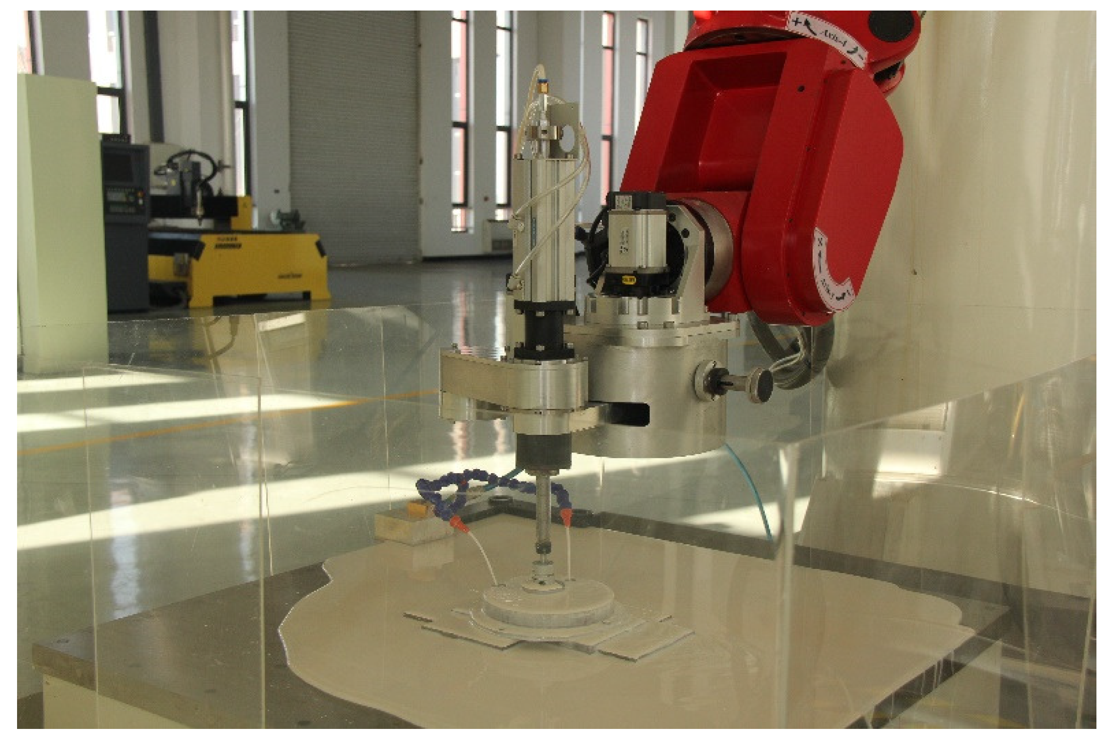
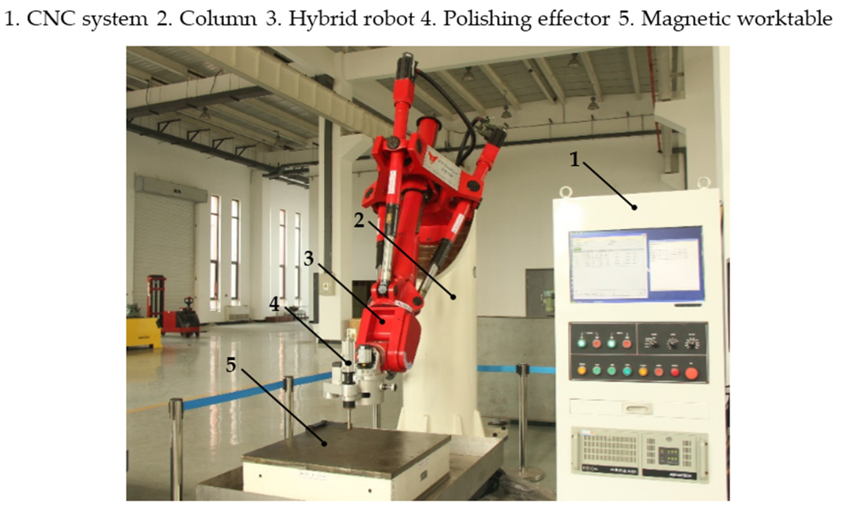
Both simulation and experiments were carried out to validate the effectiveness of the presented method on the prototype of the hybrid polishing robot. As shown in Figure 2, it is mainly composed of a 6-DOF (degrees of freedom) hybrid robot, a polishing effector, a magnetic worktable, a column, and a CNC system. The hybrid robot is composed of a 3-DOF (3UPS and UP) parallel mechanism and a 3-DOF wrist. The UP limb and the wrist form a UPS or UPRRR limb. Here, R, U, S, and P represent, respectively, revolute, universal, spherical, and prismatic joints, and the underlined P, S, and R denote the actuated prismatic, spherical, and revolute joints, respectively. The CNC system is built upon an IPC+PMAC open architecture, consisting of a host control computer responsible for reconstruction of the parametric curves, trajectory interpolation, and NC command generation, and a PMAC motion controller for servo-control of the actuated joints.

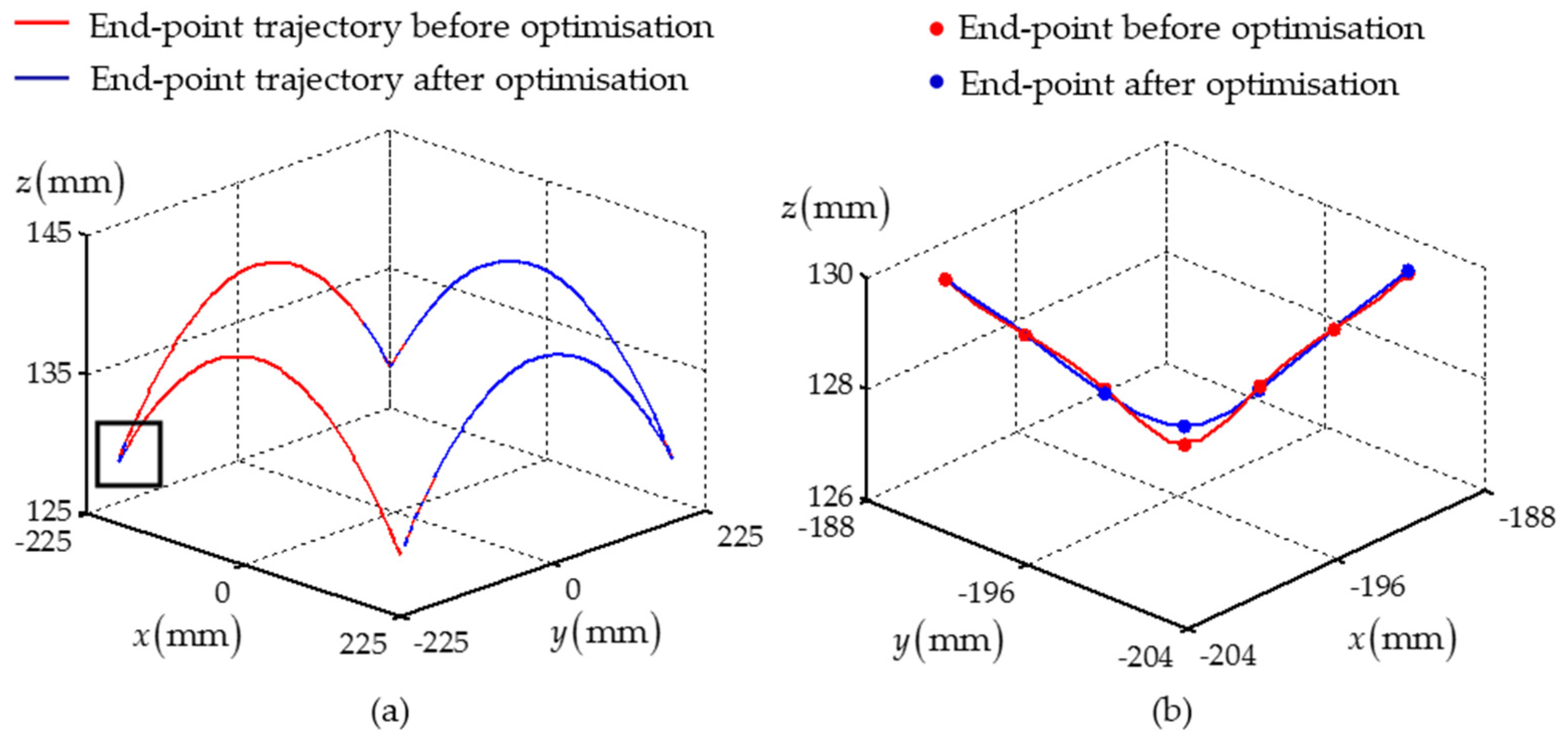
Without loss of generality, a segment of NC codes was taken from the polishing trajectory to validate the effectiveness of the proposed interpolation method. According to the SOR iterative scheme mentioned in Section 2, Figure 3 shows the two fitted trajectories. Then, the optimisation algorithm described in Section 3 is used to smooth the curvature of the trajectory. The change threshold of curvature for judging outlier points is given as 0.01. As shown in

Table 1. Changes in the two trajectories before, and after, fairing optimisation.

Trajectory	Before		After
	Maximum Curvature	Maximum Shear Jerk	Maximum Curvature	Maximum Shear Jerk
End-point	1.249	0.285	0.253	0.025
Reference-point	1.380	0.325	0.506	0.032

, the fairness of the two trajectories is both significantly improved. The maximum curvatures of the two trajectories are reduced by as much as 79.7% and 63.3% and the maximum absolute values of shear jerks are decreased by 91.2% and 90.2%, correspondingly. Considering the optimisation and interpolation methods for the two trajectories are same, experimental results of the end-point trajectory are just shown in the following discussion for the sake of simplicity.

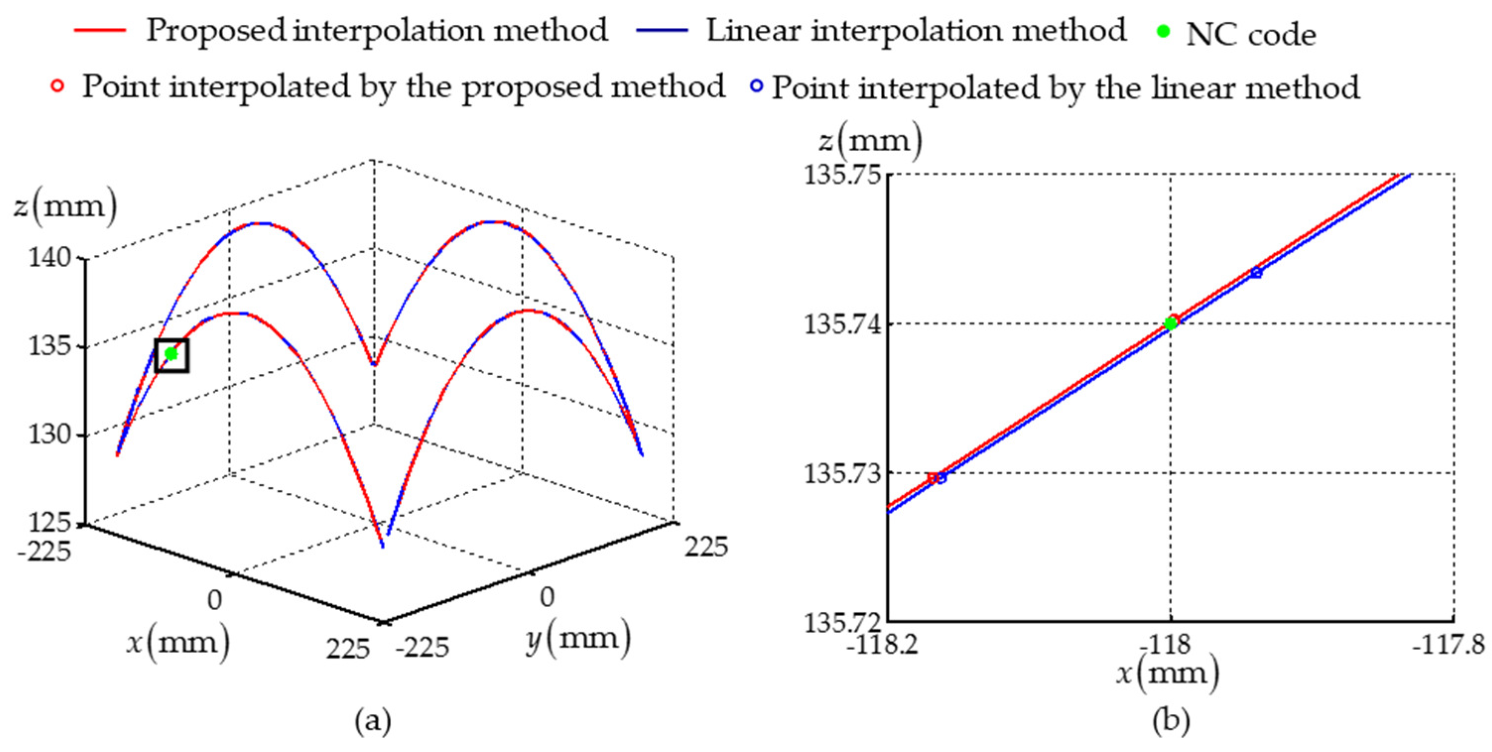
Based on the optimisation trajectory shown in Figure 4, the discrete NC command sequences were generated and sent to the PMAC motion controller, which were mapped into the servo-command of actuated joints through an inverse kinematic model. The PMAC motion controller synchronously gathered the positions and velocities fed back from the servo-motors. The interpolation and sampling periods are 10 and 20 ms, respectively. To validate the effectiveness of the method, a comparison experiment was carried out utilizing the linear interpolation method. Figure 5 shows the experimental result, which is computed by the feedback positions of all the actuated joints. It can be seen from the partial enlarged view that the NC commands generated by the proposed method are closer to the NC codes than those found using linear interpolation, which means that the removal position of polishing process can be reached more accurately. 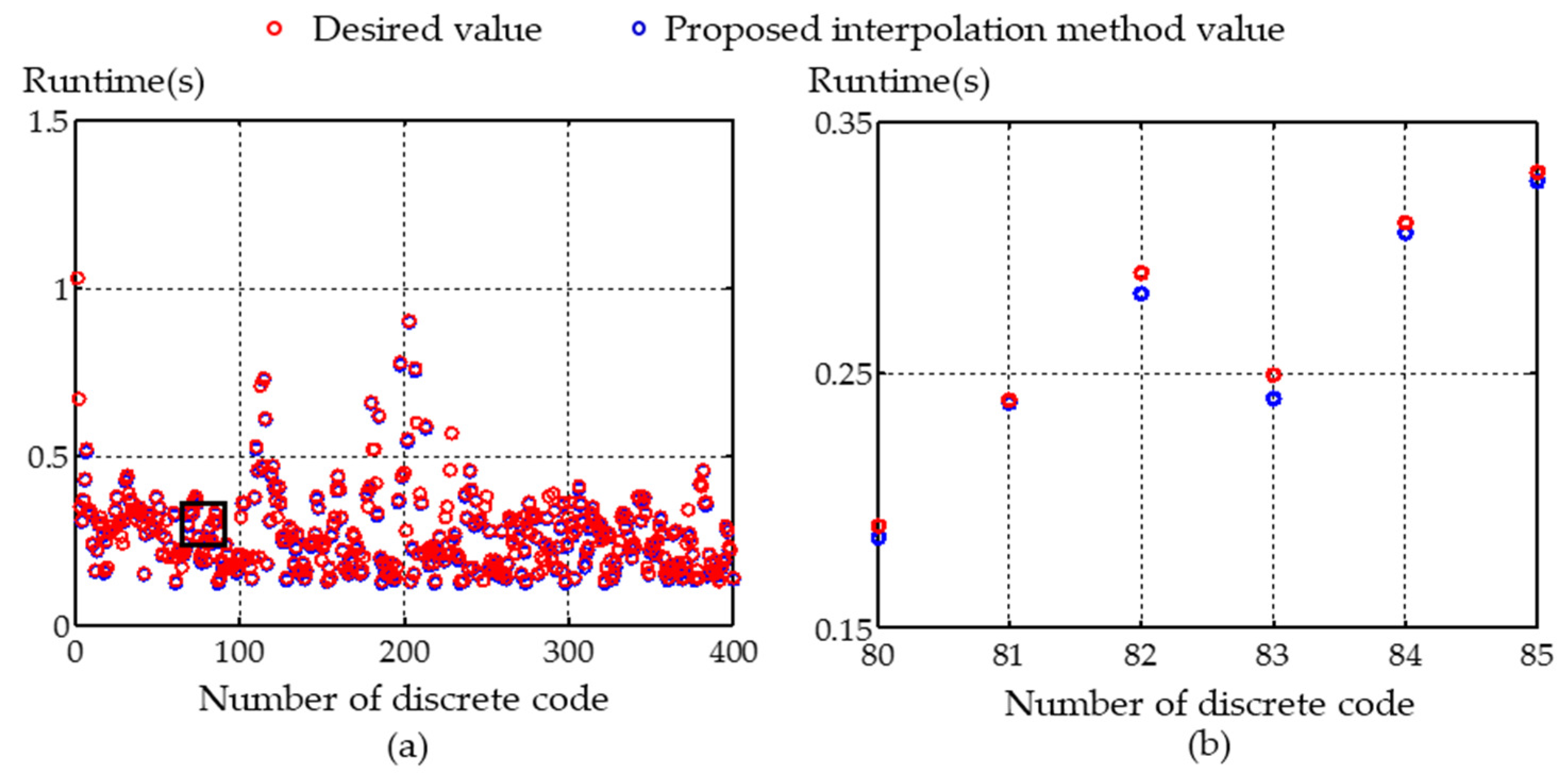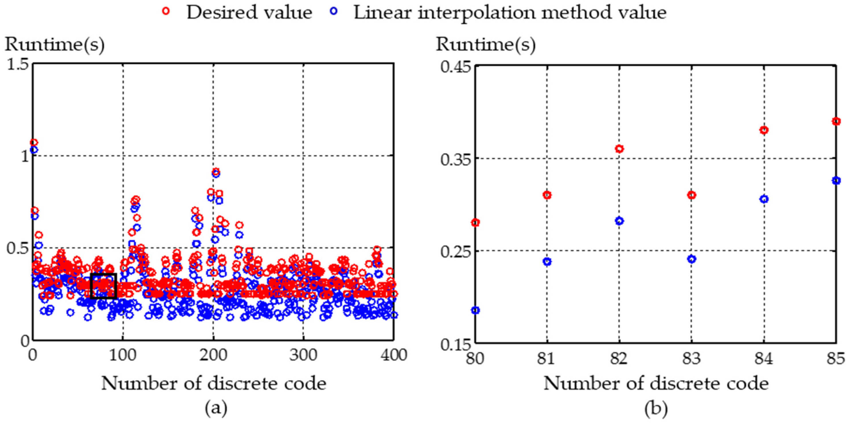Figure 6 and Figure 7 show the runtime between the adjacent NC nodes. Compared with the desired value, the proposed method is able to realise the runtime more precisely, which indicates that the removal quantity during the polishing process can be more precisely controlled, correspondingly. To evaluate the effect of the interpolation method, the indices are defined as the interpolation error ($e_i$) and the runtime error of the trajectory ($e_t$):

$$e_i={\Vert C_{i0}-C_i\Vert }_2,\hspace{0.17em}i=1,2,\dots ,n$$

(38)

$$e_{ti}=\left|t_{i0}-t_i\right|,\hspace{0.17em}i=1,2,\dots ,n$$

(39)

where $C_{i0}$ and $C_i$ denote the ith desired NC code and actual NC code after interpolation, $t_{i0}$ and $t_i$ denote the desired runtime and the actual runtime between the i − 1th and ith NC codes. It can be seen from

Table 2. Comparison of the effect of the two interpolation methods.

Method	Interpolation Error (mm)		Runtime Error (s)
	Maximum	Mean	Maximum	Mean
Proposed	0.005	0.002	0.010	0.005
Linear	0.091	0.076	0.130	0.076

that, compared to the linear interpolation method, the interpolation error and the runtime error generated through the proposed method are an order of magnitude smaller. These data further imply that the proposed interpolation method has more precision than the linear interpolation method in the polishing process.

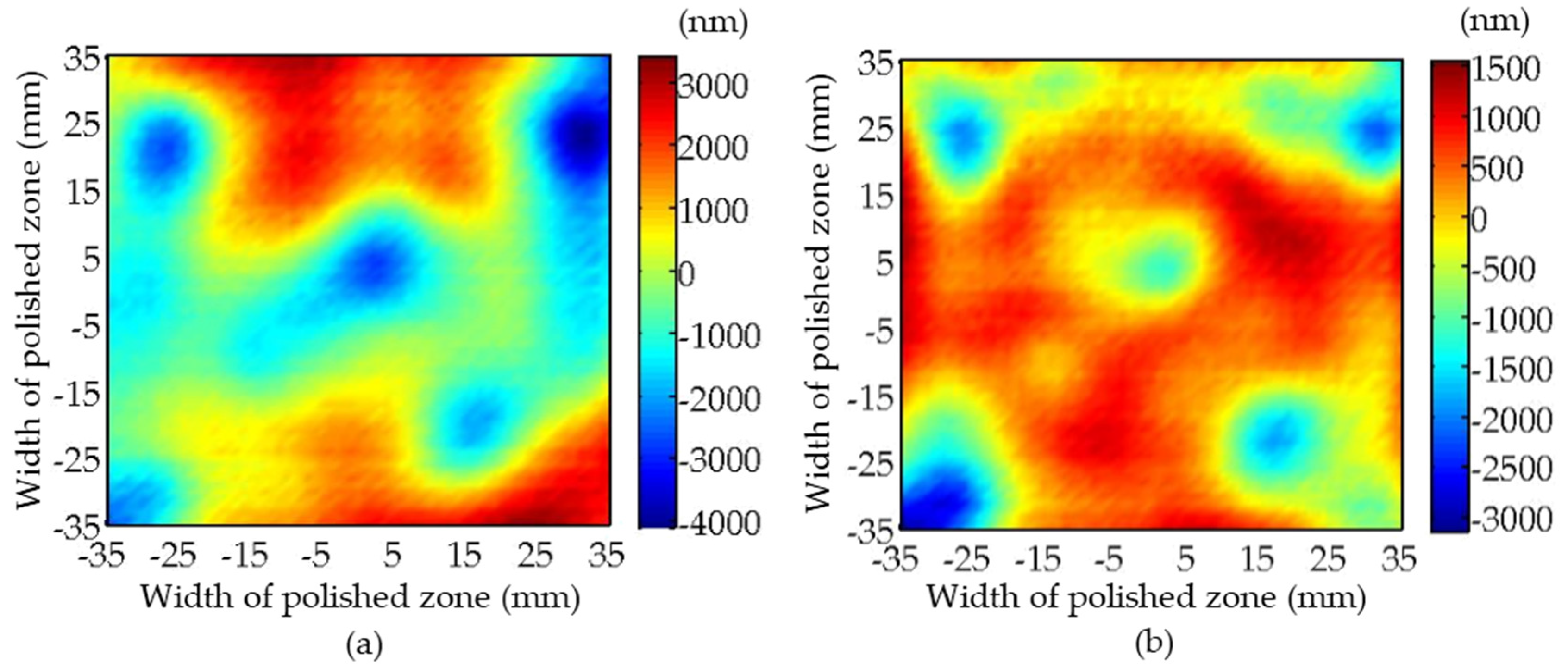
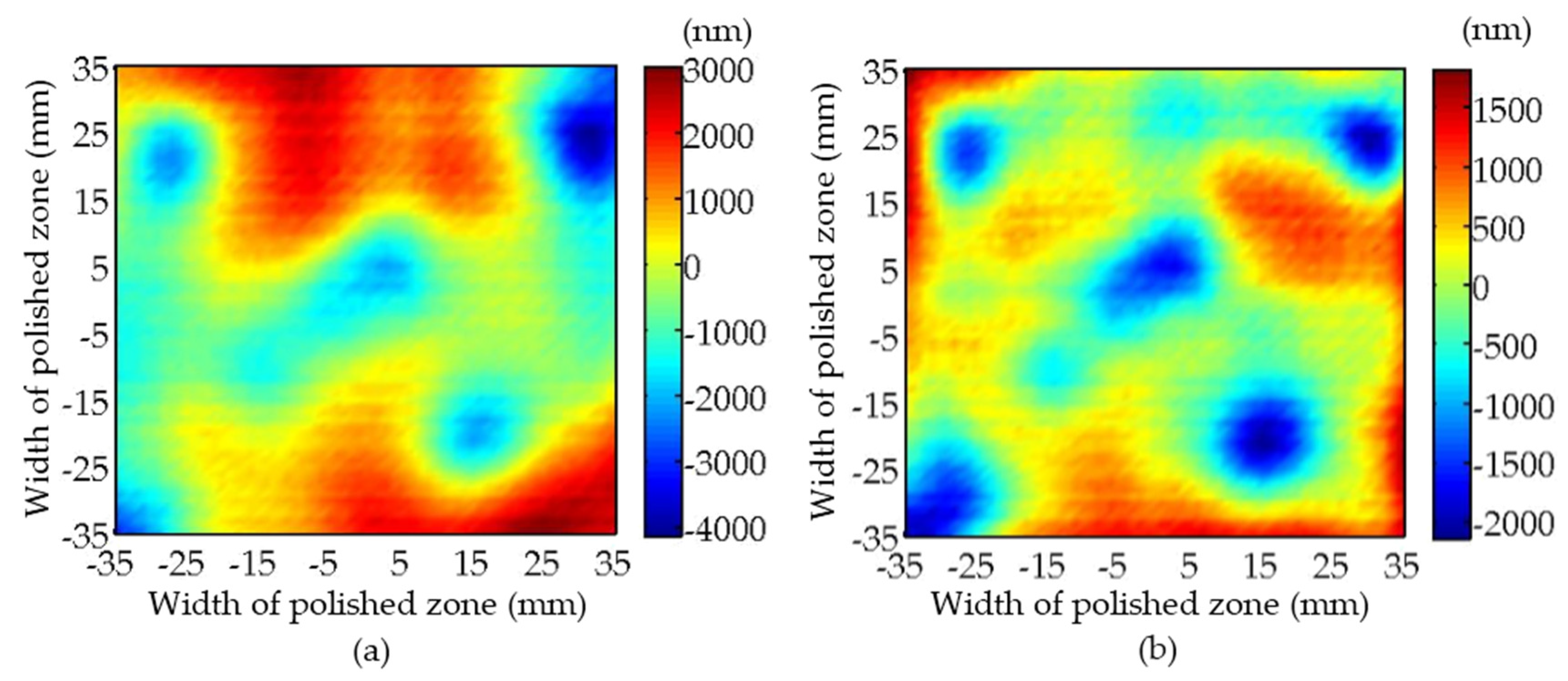
To validate the modification effect of the interpolation method on the surface error of optical elements, polishing experiments were carried out on fused silica elements by, respectively, using the linear interpolation method and the proposed interpolation method, as shown in Figure 8. Using the Nanovea contour graph, the polished zone (70 mm × 70 mm) of the elements was detected. The experimental results obtained using the two interpolation methods are displayed in Figure 9 and Figure 10, respectively. It can be seen, from the figures, that, after conducting linear interpolation-based polishing, the surface error (PV) decreases from $11.894\lambda \left(\lambda =633\mathrm{nm}\right)$ to $7.422\lambda$. In contrast, using the proposed interpolation method, the surface error (PV) is reduced from $11.282\lambda$ to $6.267\lambda$. The convergence rate of the surface error is increased from 37.59% to 44.44%, which further verifies the effectiveness of the proposed method.

6. Conclusions

A new trajectory planning method for optical polishing is proposed in this paper. It is developed to generate NC commands that can decrease the interpolation error and the runtime error. First, to obtain the NURBS trajectory without loss of the information about the runtime, a global fitting method is presented based on SOR iteration theory to deal with the problem of the computational burden arising from the large quantity of NC codes for polishing. Then, taking the shear jerk of the NURBS as the evaluation index, a fairing optimisation method is carried out to smooth the curvature saltation of the trajectory. Finally, the feed-rate planning method and the path interpolation scheme are proposed to reduce the realisation error of the trajectory runtime.

Simulation results verify that the fairing optimisation proposed in this research can modify the curvature saltation at the expense of trajectory accuracy compared to the given NC codes; however, the curvature saltation only occurs at the turning point of the trajectory and the trajectory error magnitude generated by the optimisation algorithm is consistent with the linear interpolation. Therefore, the trajectory accuracy is not treated as the index with which to evaluate the smoothing effect in Section 5. The effect of the optimisation algorithm on the optical polishing will be investigated in future work.

It can be seen from Figure 5, Figure 6 and Figure 7, and Table 2, that the runtime error of the proposed interpolation method arises because the trajectory runtime cannot be divided exactly by the interpolation period and is rounded up to an integer. In contrast, the runtime error of the linear interpolation method arises as a result of the acceleration and deceleration that occurs frequently between adjacent short line segments. Similar to the runtime error, the interpolation error of the proposed interpolation method is a result of the numerical calculation error of the trajectory length and that of the linear interpolation method is due to the transition for the discontinuity of the adjacent short line segments. Then the convergence rate of the surface error is increased with the help of the improvement in the interpolation, and runtime, errors, validating the effectiveness of the proposed interpolation process. For the aforementioned error, their individual effects on the optical polishing need to be further indicated in future work.