Feature of Echo Envelope Fluctuation and Its Application in the Discrimination of Underwater Real Echo and Synthetic Echo

1
School of Naval Architecture, Dalian University of Technology, Dalian 116024, China
2
Science and Technology on Underwater Test and Control Laboratory, Dalian 116013, China
*
Author to whom correspondence should be addressed.
Appl. Sci. 2018, 8(8), 1329; https://doi.org/10.3390/app8081329
Submission received: 3 June 2018
/
Revised: 20 July 2018
/
Accepted: 7 August 2018
/
Published: 9 August 2018
(This article belongs to the Section Acoustics and Vibrations)
Abstract
:Discriminating a real underwater target echo from a synthetic echo is a key challenge to identifying an underwater target. The structure of an echo envelope contains information which closely relates to the physical parameters of the underwater target, and the characterization and extraction of echo features are problematic issues for active sonar target classification. In this study, firstly, the high-frequency envelope fluctuation of a complex underwater target echo was analyzed, the envelope fluctuation was characterized by the envelope fluctuation intensity, and a characterization model was established. The features of a benchmark model echo were extracted and analyzed by theoretical simulation and sea testing of a scaled model, and the result shows that the envelope fluctuation intensity varies with carrier frequency and azimuth of incident signal, but the echo envelope fluctuation of the synthetic target echo does not present these features. Then, based on the characteristics of echo envelope fluctuation, a novel method was developed for active sonar discrimination of a real underwater target echo from the synthetic echo. Through a sea experiment, the real target echo and synthetic echo were classified by their different echo envelope fluctuations, and the feasibility of the method was verified.
1. Introduction
An active acoustic decoy which can simulate a target echo provides very important countermeasures to active acoustic torpedoes and active sonar. Basically, the active acoustic decoy comprises several monostatic hydrophones, and once the hydrophones receive the incident sonar pulse, the monostatic hydrophones transmit an acoustic wave with a certain phase, magnitude, Doppler frequency shift, time delay, and signal broadening that characterize the target echo [1,2,3,4]. This kind of active acoustic decoy can simulate a series of an echo’s characteristic parameters, such as the relative positions of the main echo highlights, relative magnitude of echo highlights, and scale features of the target, and it is a great challenge for active sonar target classification.
Many algorithms have been developed for underwater acoustic target tracking [5,6,7,8], but discriminating the real underwater target echo from the synthetic echo is still a key challenge to identifying an underwater target. The echo of an underwater target is the incident signal modulated by material, structure, and shape parameters, so the echo envelope structure is the characterization of the target’s geometric scattering and elastic scattering in a time domain [9,10,11,12]. Therefore, the envelope structure of an underwater echo contains the information which closely relates to the physical parameters of the target. In a high-frequency acoustic scattering wave, the echo’s energy is dominated by a geometrical scattering wave, the geometrical scattering highlights are always present in the high-amplitude fluctuation of an echo envelope, while the elastic scattering highlights are present in the fast and weak fluctuation of the envelope [13].
For the high-amplitude fluctuation of an echo envelope, the envelope’s structural features can be characterized by the number of echo highlights, relative magnitude, and relative spacing [14,15,16,17,18]. A statistical quantitative model of echo highlights has been established for a complex target, which quantitatively characterizes the echo highlights [19]. For the weak fluctuation of the echo envelope, which contains the elastic scattering, for an actual echo signal, the features of weak fluctuation echo envelope are hard to extract and use [13].
In previous work, echo envelope fluctuation features were studied in a frequency domain, and the envelope modulation rate of underwater target’s scattering signal is characterized. Theoretical and experimental research has indicated that the maximum envelope modulation frequency of a complex target increases when the incident frequency increases [20]. Based on the maximum envelope modulation frequency, a method for discriminating the real target from the synthetic target was proposed and tested [21]. The maximum envelope modulation frequency was obtained by using a threshold for the strong influence of low-frequency envelope modulation. The extraction of maximum frequency is always affected by the threshold, and the correct choice of the threshold is often not easy for actual sea data. Consequently, in order to deeply understand the mechanism of echo envelope modulation and to properly describe the echo envelope fluctuation, the authors studied the features of echo envelope fluctuation in a time domain, and they proposed a novel method for the discrimination of a real underwater target echo from a synthetic echo. Compared with previous work, the strong influence of a low-frequency echo envelope fluctuation was reduced, the fine structure of a high fluctuation envelope was enhanced, and the processing of the features extracted from a high-frequency modulation was straightforward.
The major contributions of this paper are as follows:
- This paper focuses on the characterization and extraction of echo fluctuation features from an underwater complex target. Based on practical engineering applications, it presents a method for discrimination of a real echo from a synthetic echo underwater.
- The high-frequency fluctuation of an echo envelope was characterized by the echo envelope fluctuation intensity, and a model of echo envelope fluctuation intensity was established.
- Results from simulation and real sea experiments of a benchmark model and synthetic echo are provided in detail.
- The feasibility of the proposed method for discriminating between a real target echo and a synthetic echo was verified by real sea experiment. The method proposed in this paper has low processing complexity and provides a new and valuable insight into the classification of underwater real and synthetic echoes.
The rest of this paper is organized as follows. Section 2 describes the theoretical analysis of the high-frequency envelope fluctuation of a complex underwater target echo, and the characterization model we established is presented. Section 3 presents the extraction of echo envelope fluctuation features from a scaled benchmark model and synthetic echo with different frequencies and pulse lengths, and the simulation and experimental results are discussed in detail. Section 4 describes the proposed method of real echo and synthetic echo discrimination. Section 5 consists of sea experiments, data processing results, and discussion of estimation performance. A summary of the proposed method is provided in Section 6.
2. Characterization of Echo Envelope Fluctuation Features
2.1. Relation of Echo Envelope Fluctuation with Carrier Frequency of Incident Pulse
Normally, based on the echo highlight model, an echo is considered the superposition of echo highlights and background. In this study, the concept underlying the echo highlight model has been generalized: the echo is the supposition of highlights from scatterings on the target, and the scatterings are equally spaced according to the carrier frequency of the incident pulse. For the linear dimension, the complex echo can be expressed by [20]
where is the azimuth of the incident signal; is the strength coefficient of the echo highlight, assumed equal spaced distribution of scatter on the target; is the incident signal; is the number of echo highlights; is the difference in time between the echo highlight and the start of the echo signal, i.e.,
where is the length of the target, is the sound speed in water. Assuming equal strength coefficients of echo highlights, namely , the frequency domain expression of (1) is as below [21]
where
In (3) and (4), receives the maximum value when . The echo envelope forms dips and peaks correspondingly. As per the theoretical expression above, the spacing of echo highlights relates to the carrier frequency, and when the carrier frequency increases, a higher frequency modulation of the echo envelope forms, presenting more detailed information on the target. It also implies that when the carrier frequency changes, the characteristics of the echo envelope modulation change accordingly, representing the features of a real complex target.
2.2. Characterization of Underwater Target Echo Envelope Fluctuation Intensity
A high-frequency fluctuation of the echo envelope represents the fine features of an underwater complex target echo, but the energy of a low-frequency fluctuation of the echo envelope dominates the whole echo envelope. Normally, extracting the features from a high-frequency fluctuation of the echo envelope is not easy. The maximum fluctuation frequency could be used to characterize the high-frequency envelope fluctuation and its features extracted in the frequency domain [20], but the maximum envelope modulation frequency is obtained by using a threshold, and correctly choosing the threshold is difficult for actual sea data. In this work, the extraction of features from a high-frequency fluctuation of the echo envelope was carried out in the time domain.
The intensity of the magnitude of the envelope signal fluctuates with time, and it can be characterized by a differential coefficient, through differentiation of the echo envelope. The low-frequency envelope fluctuation is suppressed, equivalent to high-pass filtering, and the high-frequency envelope fluctuation is enhanced.
For convenient analysis in the time domain, Equation (1) is expressed as
Deriving the formula, with time (t) as a variable, the echo envelope fluctuation intensity is
From this expression, the echo envelope fluctuation intensity strongly relates to the carrier frequency of the incident pulse, and the echo envelope fluctuation intensity varies with the carrier frequency accordingly.
The envelope fluctuation intensity is a time-changing value, and it cannot be used directly for discriminating between different echo signals. In this paper, the feature is characterized by two parameters, one being fluctuation intensity
where is the discrete series of , is the difference between adjacent elements of , and is the data length. is called the fluctuation intensity, which characterizes the whole fluctuation intensity of the echo envelope.
Another parameter is the standard deviation (STD) of echo envelope magnitude fluctuation intensity,
where
where characterizes the inconsistency of the fluctuation intensity of the envelope that varies with time.
3. Extraction of Echo Envelope Fluctuation Features
3.1. Simulation Study
3.1.1. Simulation Study of Benchmark
Based on the analysis above, the envelope fluctuation intensity was studied through simulation, where the target studied is the benchmark model [22] scaled by a ratio of 1:20, the length is 3 m, and the scaled model is made of steel. The incident pulse is a linear frequency modulation (LFM) signal, the frequencies are 10–20 kHz and 20–40 kHz, and the pulse lengths are 1 ms and 3 ms.
The method of echo simulation is called the frequency indirect echo simulation method. The acoustic scattering of the target can be considered a linear system or target scattering channel, the incident signal is the system input, and the echo is the system output that is transferred by the target system and underwater sound channel. In this study, the transfer function of the target was calculated using special software that is based on the planar element method (PEM)—a numerical model that converts an integral calculation to arithmetic calculation [23,24]. The software can rapidly calculate sonar echo characteristics from sonar targets of various shapes [25].
Figure 1, Figure 2 and Figure 3 are the simulated echo envelope fluctuation features. Figure 1a and Figure 2a are the echo envelope fluctuation intensities with different pulse lengths, and Figure 1b and Figure 2b are the corresponding STDs of echo envelope fluctuation with different pulse lengths.
The simulation results show that the fluctuation intensity and its standard deviation change dramatically with the azimuth, with the minimum intensity on the beam, and the maximum on the keel-line. The cause is that the time difference of the echo highlight in the keel-line is greater than that in the beam direction; correspondingly, the phase difference is larger than that causing the strong fluctuation of the echo envelope. However, in the beam direction, the phases of different echo highlights are nearly the same, and the envelope is flatter than that in other azimuths.
Figure 3 compares the fluctuation intensity features of the echo envelope for different frequencies, 10–20 kHz and 20–40 kHz, with 1 ms pulse lengths. Figure 3a is the comparison of fluctuation intensity, and Figure 3b is the comparison of STDs of echo envelope fluctuation intensity, correspondingly. The simulated results show that the echo envelope fluctuation intensity greatly depends on the carrier frequency: when the carrier frequency increases, the echo envelope fluctuation intensity increases correspondingly, which is consistent with the theoretical analysis.
3.1.2. Simulation Study of Synthetic Echo
The echo of an active acoustic decoy was simulated by several monostatic hydrophones, where the number of monostatic hydrophones represents the number of main echo highlights. In this study, the synthetic echo was simulated based on the statistical features of echo highlights [19]. The number of highlights is six; the incident pulse is the LFM signal; the frequencies are 10–20 kHz, 20–40 kHz, and 40–80 kHz; and the pulse lengths are 1 ms and 3 ms.
Figure 4 shows the results of the synthetic echo. Figure 4a compares the fluctuation intensity features of the echo envelope for different frequencies, and Figure 4b compares the STD of the echo envelope fluctuation intensity, correspondingly. The simulation results of 3 ms pulse length are consistent with Figure 4. From the results, we can see that the fluctuation intensity and its STD remain almost stable when the carrier frequencies change. This greatly differs from the results of the benchmark model because the synthetic echo is the superposition of signals from several monostatic hydrophones. The low-frequency modulation features of the echo envelope can be simulated, such as the echo highlights, but the high-frequency modulation features cannot be simulated, such as echo envelope fluctuation intensity. The high-frequency modulation features are caused by body scattering and elastic scattering.
3.2. Experiment Study of Benchmark Model and Rock
3.2.1. Experiment Configuration
For comparison with the simulation results, broadband acoustic scattering testing was conducted with the scaled benchmark model and with rock. Figure 5 shows the experiment configuration: Figure 5a is the schematic diagram of the experimental layout, Figure 5b is the photo of the sea experiment, and Figure 5c is the photo of the rock that was tested.
The target and monostatic sonar were mounted on the experimental ship, and the target was mounted by two thin ropes on the rotator, by which the azimuth was changed from 0 degree to 180 degrees. The depth of the target and monostatic sonar was 5 m deep in the water, and the range between the target and the sonar was 21 m, which satisfies the testing requirements for far field acoustic scattering. The transmitting beam was maintained on the benchmark to diminish interference from reverberation.
A continuous wave (CW) signal and a linear frequency modulation wave signal were tested; the parameters were as listed in Table 1.
3.2.2. Experimental Results
The procedure for processing the test data for the echo envelope fluctuation feature of the benchmark model is:
- Filter the data by a bandpass filter to minimize the interference;
- Calculate the envelope of the echo signal;
- Normalize the echo envelope for magnitude consistency;
- Differentiate the echo envelope;
- Calculate the fluctuation intensity and the standard deviation;
- Process the echo in whole azimuths.
Figure 6a is the echo envelope with LFM 20–40 kHz at a certain azimuth, and the pulse length is 1 ms; Figure 6b is the echo envelope fluctuation after differentiation; Figure 7a is the echo envelope with LFM 40–80 kHz, the pulse length is 1 ms; and Figure 7b is the echo envelope fluctuation after differentiation. Results show that, after differentiation, the energy of geometric scattering has decreased, and the fine structure of the high fluctuation envelope has been enhanced.
Then, the echo data in whole azimuths were processed, and the echo envelope fluctuation features with varied carrier frequency, pulse length, and azimuth were analyzed.
A. Fluctuation Intensity
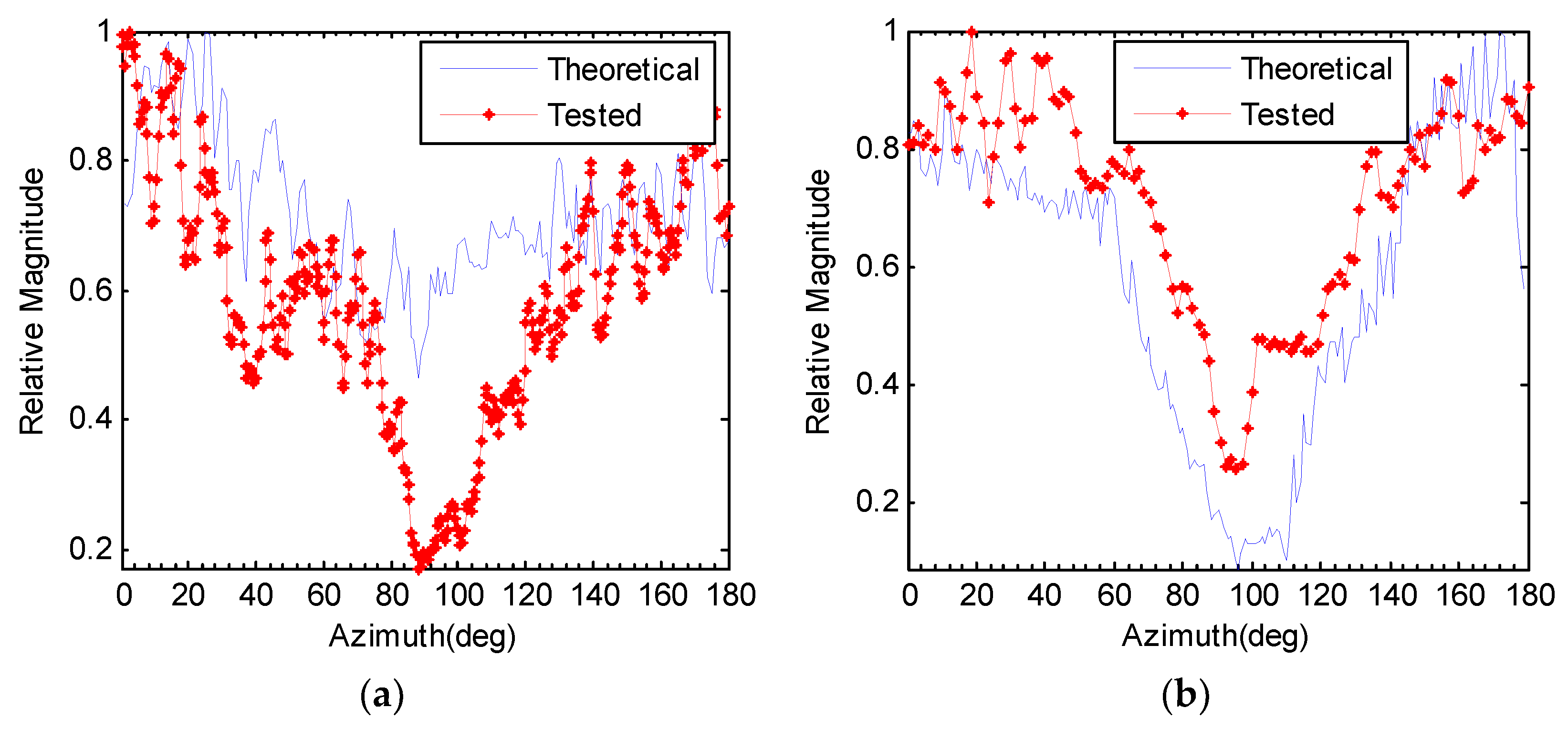
Figure 8 is the comparison of fluctuation intensity for experimental and simulated results for a frequency of LFM 20–40 kHz and pulse lengths of 1 ms and 3 ms, respectively. Figure 8 shows that the tendencies of the experimental and simulated results are fundamentally similar; the value of the fluctuation intensity is at the minimum on the beam, and at the maximum on the keel-line.
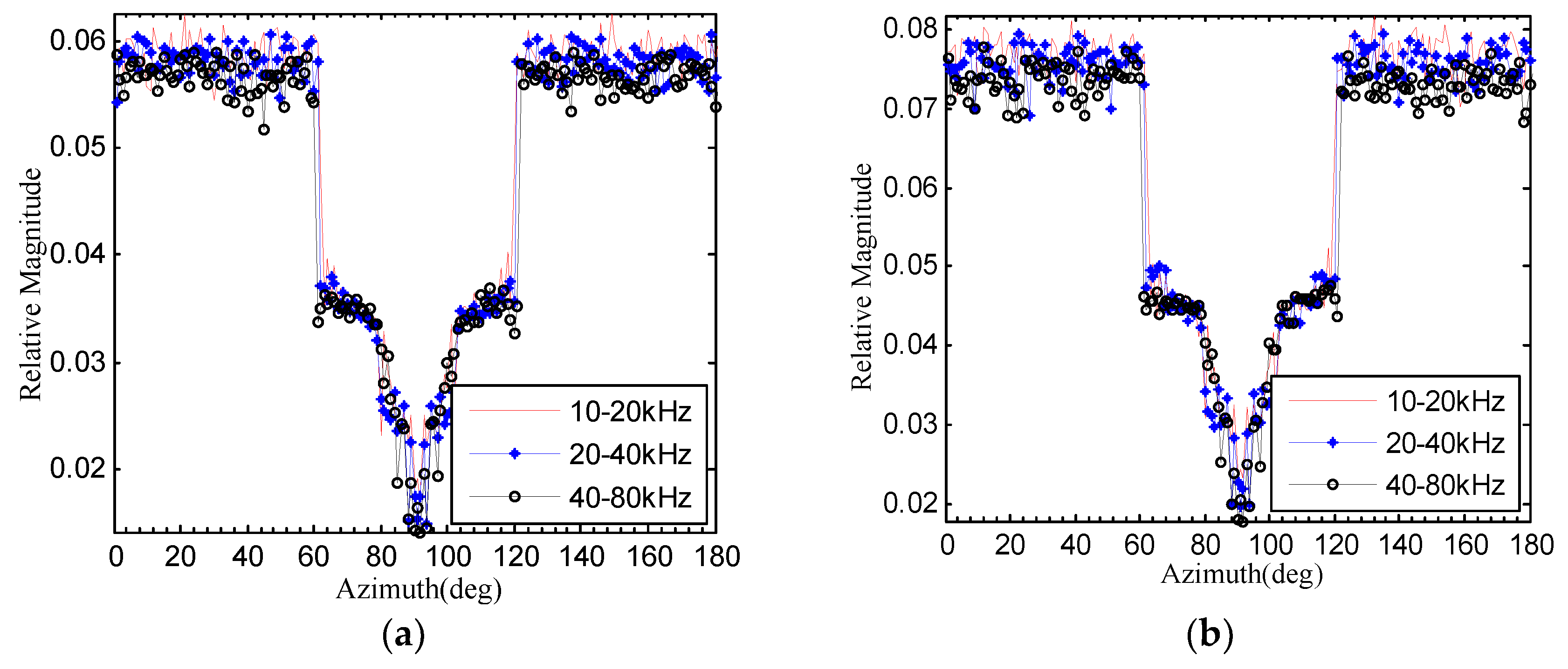
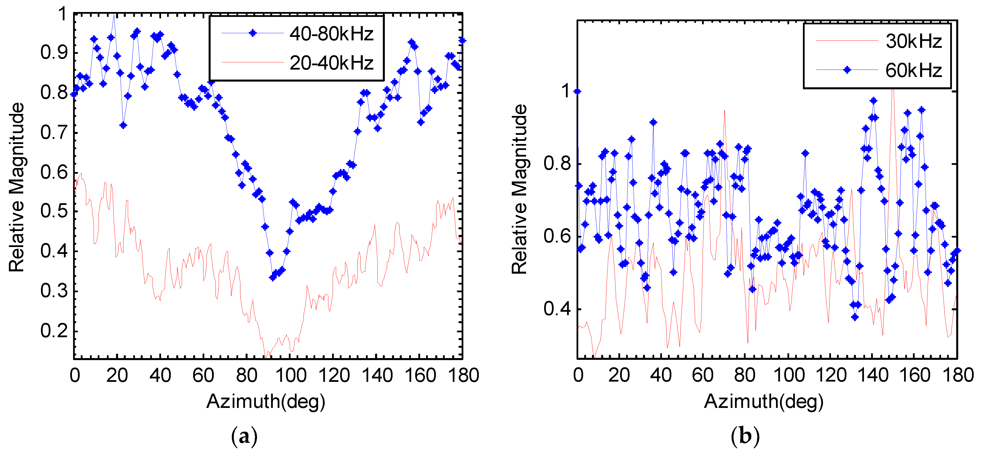
Figure 9 is the fluctuation intensity results of the scaled benchmark model with different carrier frequencies: the tested signal from Figure 9a is the broadband signal, and Figure 9b is a single frequency signal. From the results, we can see that the echo envelope fluctuation intensity greatly depends on the carrier frequency; when the carrier frequency increases, the echo envelope fluctuation intensity increases correspondingly. According to the theoretical analysis, when the carrier frequency increases, the time resolution of the incident pulse increases, the echo envelope presents a finer fluctuation, and the fluctuation intensity of the envelope increases correspondingly. This feature notably represents the influence of target shape and structure on the echo envelope.
From the comparison of Figure 9a,b, we can see that the echo envelope fluctuation intensity of the narrowband signal does not change markedly compared to that of the broadband. This is because the time resolution of the broadband signal is greater than that of the narrowband signal, thus, the envelope structure presents a higher frequency fluctuation.
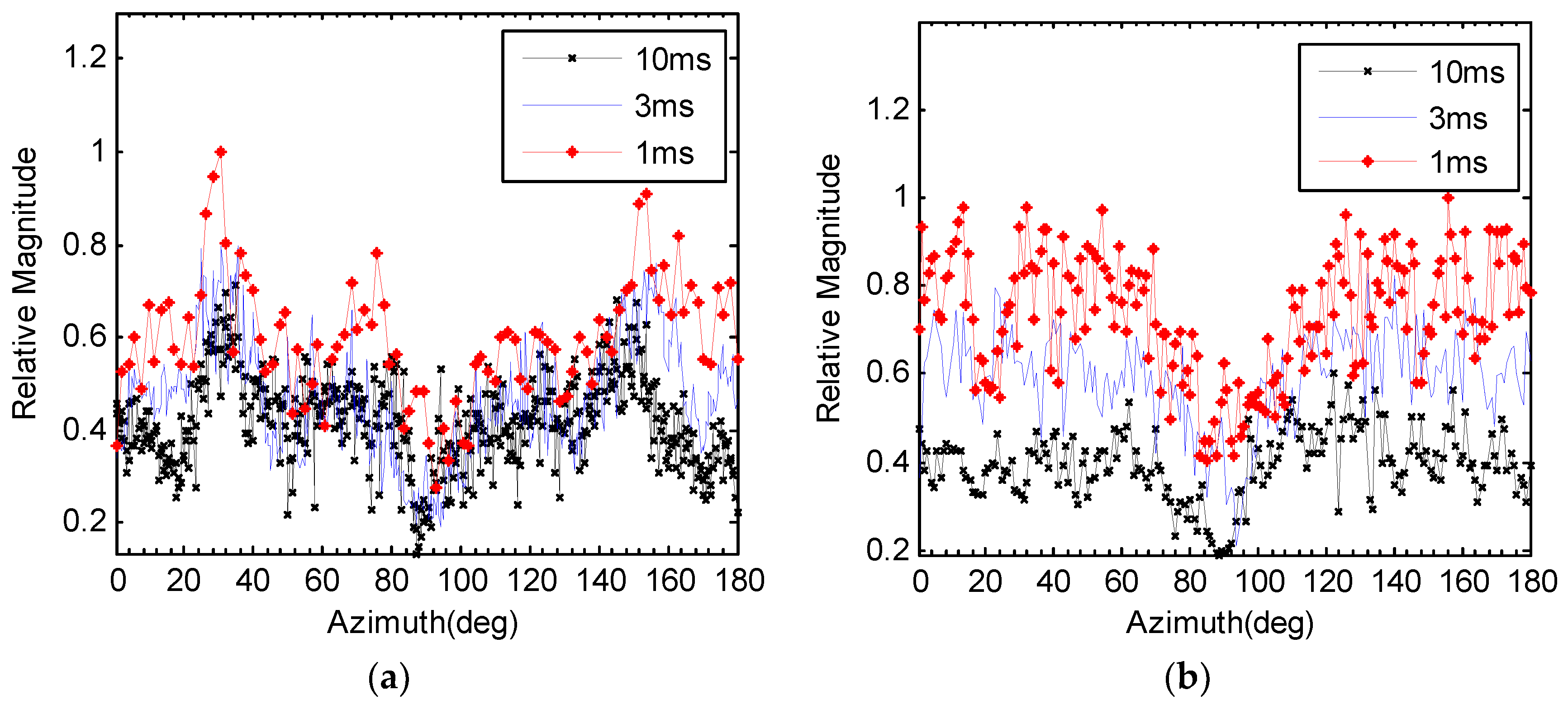
Figure 10a,b is the echo fluctuation intensities of the CW and LFM signals, with pulse lengths of 1, 3, and 10 ms, respectively. The results show that the magnitude of the fluctuation intensity changes as the pulse length changes; when the pulse length increases, the magnitude of the echo fluctuation intensity decreases. This is because a smaller pulse length has a greater time resolution, the echo envelope presents finer fluctuation, and, correspondingly, the fluctuation intensity of the envelope increases. This feature is consistent with the theoretical analysis. Also, as shown in Figure 9, the wideband signal provides better time resolution than that of the narrowband signal. Then, the envelope structure presents a higher frequency fluctuation, so the wideband pulse presents clearer results than the narrowband signal with the same pulse length.
B. Standard Deviation of Fluctuation Intensity
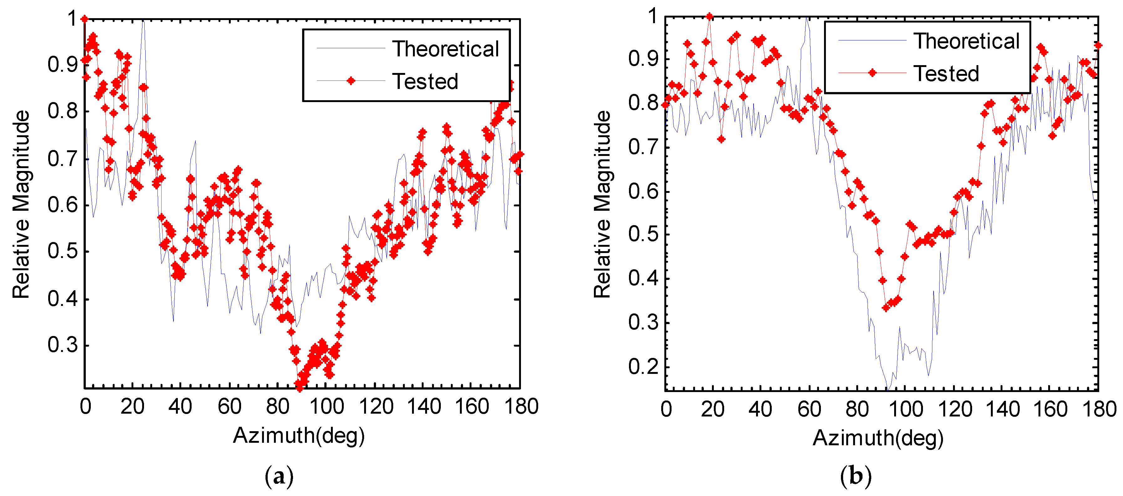
Figure 11 compares the STDs of the theoretical and experimental echo envelope fluctuation intensities with LFM 20–40 kHz and pulse lengths of 1 ms and 3 ms, respectively. Figure 11 shows that the tendency of the experimental and simulated results are fundamentally similar: the STD of the fluctuation intensity is minimum on the beam, and maximum on the keel-line.
Figure 12 is the STD results of fluctuation intensity of the scaled benchmark model, varying with azimuth: Figure 12a shows the results of the broadband signal, and Figure 12b shows the results of the narrowband signal. The results of the two kinds of tested signals show that the standard deviation of the fluctuation intensity depends on the carrier frequency; it increases with increasing carrier frequency, and it is more notable for the broadband signal—similar to the fluctuation intensity results. Compared with the fluctuation intensity of the narrowband signal, the narrowband signal’s standard deviation of fluctuation intensity changes with carrier frequency, and these changes are relatively weak. The resolution performance of this feature is not notable.
C. Envelope Fluctuation Features of Rock
For further study, we tested the rock with frequencies of 43–47 kHz and 71–74 kHz, and a pulse length of 1 ms. Figure 13a is the fluctuation intensity comparison of the rock echo envelope with different frequencies; Figure 13b is the STD comparison of the rock echo envelope fluctuation intensity with different frequencies. The results of the test with the rock show that the echo envelope fluctuation intensity and its STD increase correspondingly when the carrier frequency increases, which further verifies the theoretical analysis.
4. Method of Real Echo and Synthetic Echo Discrimination
Normally, the synthetic echo that is simulated by an active sonar decoy is synthesized by the signal that is transmitted from several monostatic hydrophones. The number of hydrophones is determined by the number of predominant echo highlights, which are characterized by the relative spacing of the hydrophones and the relative magnitude of the transmitted signal. For a real sonar decoy, the number of hydrophones is fixed, the high-frequency echo envelope modulation characteristics (such as echo envelope fluctuation intensity) cannot be simulated, and the echo envelope fluctuation intensity changes with frequencies.
Based on these echo envelope fluctuation characteristics, a novel method was developed for the discrimination of real underwater target echoes from synthetic echoes. The procedure is as below:
a. The active sonar transmits two different frequency pulses with frequency and (LFM signal is preferred), and the difference will be notable;
b. Filter the input data by a bandpass filter to minimize the interference;
c. Processing the envelope data for the two different frequency echoes;
d. Extract the envelope fluctuation features for the two different frequency echoes, such as echo envelope fluctuation intensity;
e. Compare the fluctuation features, and then discriminate between the real underwater target echo and the synthetic echo.
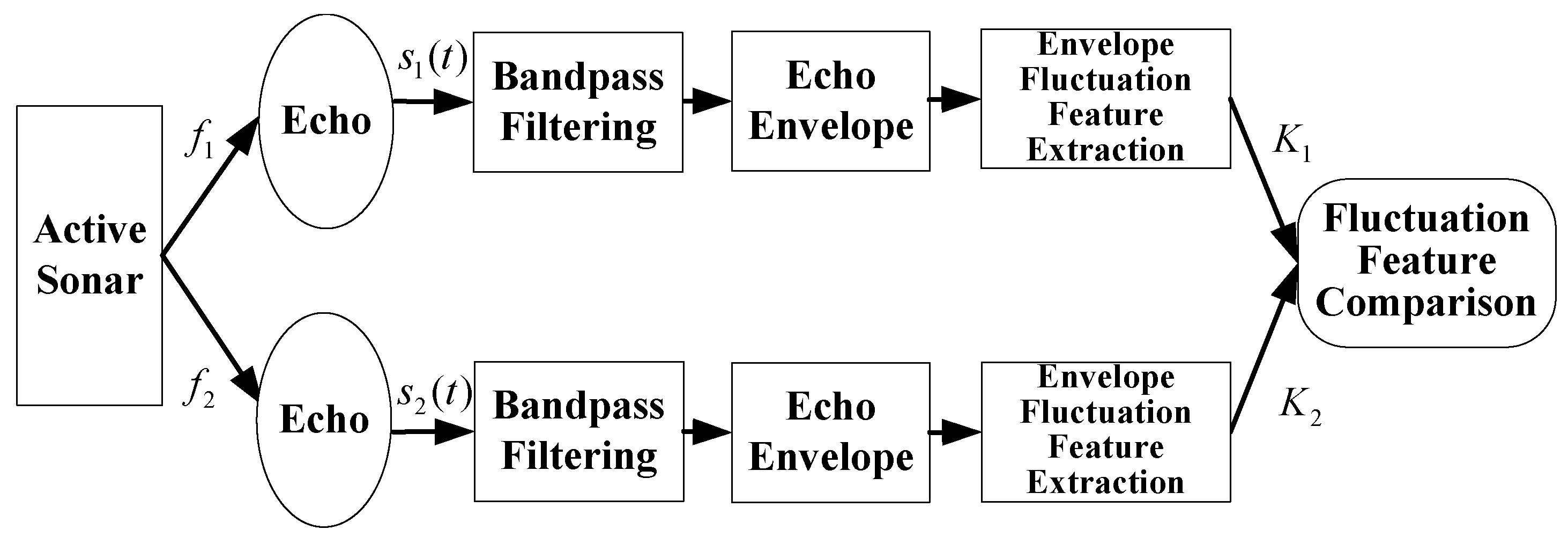
Figure 14 is the proposed procedure for discriminating a real underwater target echo from a synthetic echo.
5. Experimental Results
In order to further verify the feasibility of the proposed method, the research team carried out a sea experiment in the sea near Dalian, China. The sea area is at a depth of 30–40 m, and it has fine sediment. Figure 15 is the configuration of the synthetic echo test. The echo was simulated by two monostatic hydrophones, where the spacing between the two hydrophones was 1.4 m. By rotating the pole that mounted the two hydrophones, the azimuth of the echo was changed from 0 degree to 180 degrees. The receiver and transmitter were mounted on the experimental ship. The receiver and transmitter were 5 m deep in the water. The 20–40 kHz and 40–80 kHz LFM wideband signals were tested using pulse lengths of 1 ms and 3 ms.
Figure 16 is the synthesized echo envelope with LFM 20–40 kHz and an azimuth of 45 degrees, and the results after differentiation. Figure 17 is the simulated echo envelope with LFM 40–80 kHz and an azimuth of 45 degrees, and the results after differentiation. From the comparison of Figure 16a and Figure 17a, we can see that the shape and structure of the echo envelope remains almost the same when the carrier frequency changes, and the gradient of the echo envelope differs slightly. For the real target echo, from the comparison of Figure 6a and Figure 7a, the shape and structure of the echo envelope differ notably when the carrier frequency changes, as does the gradient of the echo envelope.
The echo in all azimuths was processed, and the echo envelope fluctuation features for the two different frequencies were extracted.
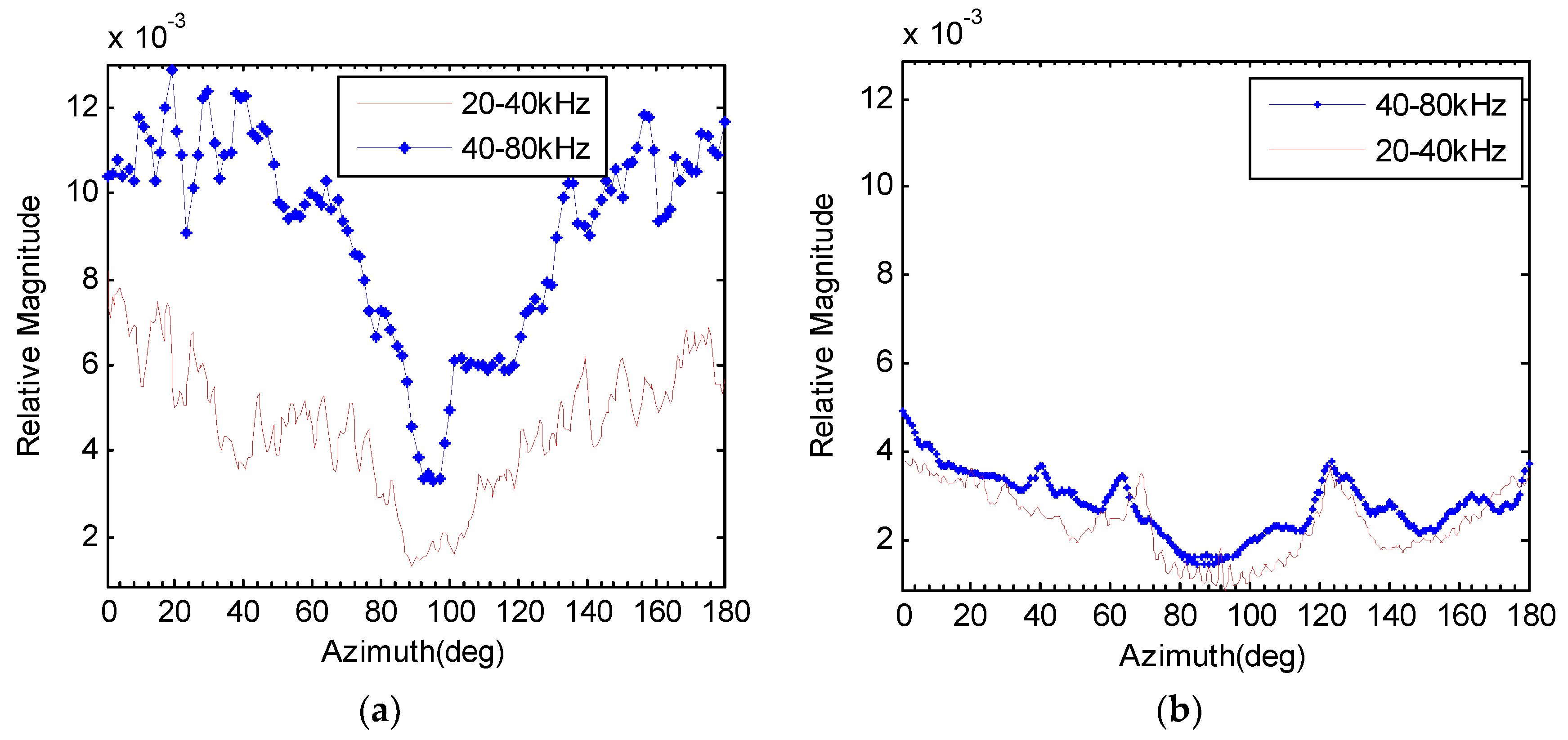
Figure 18 is the fluctuation intensity of the real target echo and the synthetic echo of the wideband echo envelope for different frequencies, with a pulse length of 1 ms. Figure 18a is the fluctuation intensity comparison of the real target’s wideband echo envelope for different frequencies; Figure 18b is the fluctuation intensity comparison of the synthetic wideband echo envelope for different frequencies.
Figure 19 is the standard deviation of the fluctuation intensity of the real target echo and the synthetic echo of the wideband echo envelope for different frequencies, where the pulse length is 1 ms. Figure 19a compares the standard deviation of the fluctuation intensity of the real target’s wideband echo envelope for different frequencies; Figure 19b compares the standard deviation of the fluctuation intensity of the synthetic wideband echo envelope for different frequencies.
Figure 20 is the fluctuation intensity of the real target echo and the synthetic echo of the wideband echo envelope for different frequencies, where the pulse length is 3 ms. Figure 20a is the fluctuation intensity comparison of the real target wideband echo envelope for different frequencies; Figure 20b is the fluctuation intensity comparison of the synthetic wideband echo envelope for different frequencies.
From Figure 18, Figure 19 and Figure 20, we can see that the fluctuation intensity and its STD of the real target echo changes notably when the carrier frequency changes, but the fluctuation intensity and its STD of the synthetic echo remains almost the same when the carrier frequency changes. The experimental results are consistent with the theoretical analysis and simulation results.
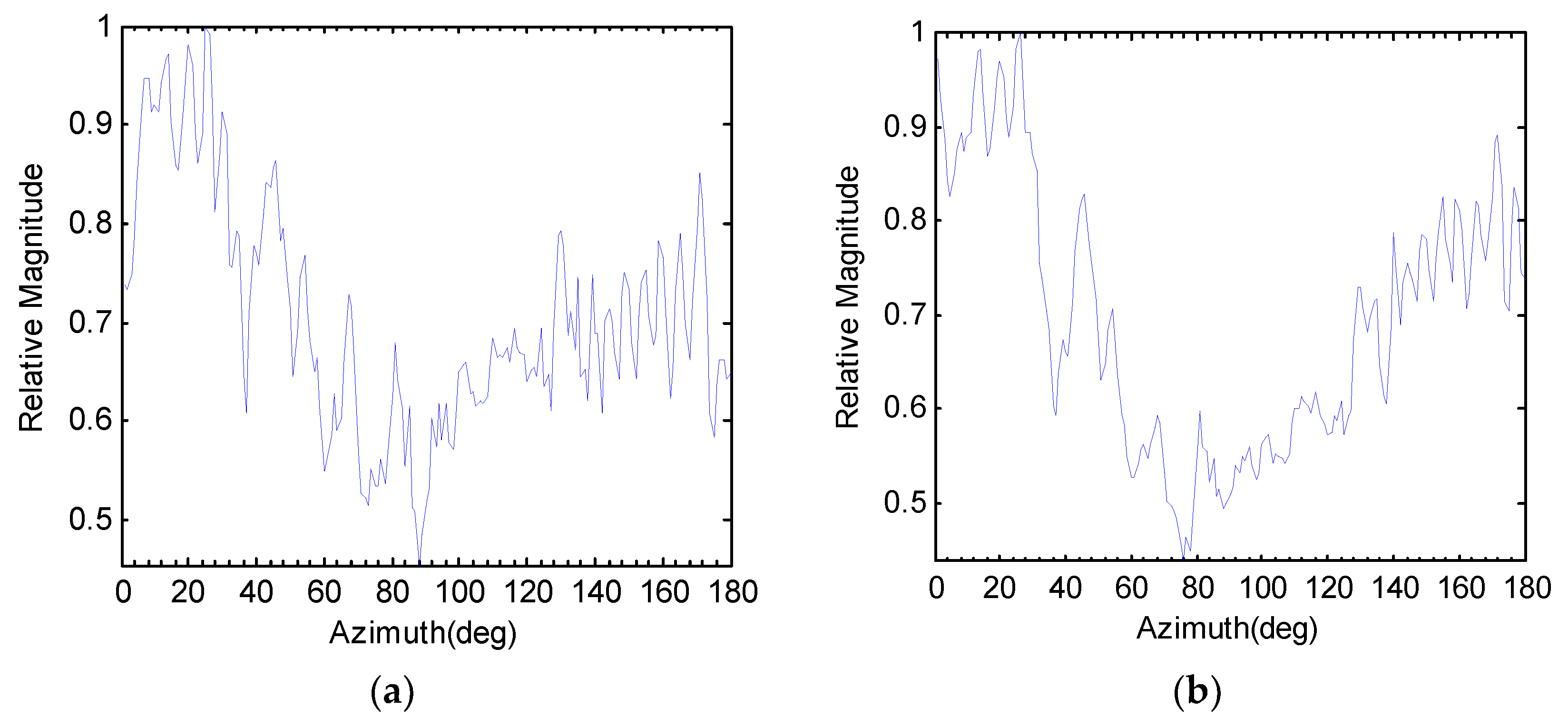
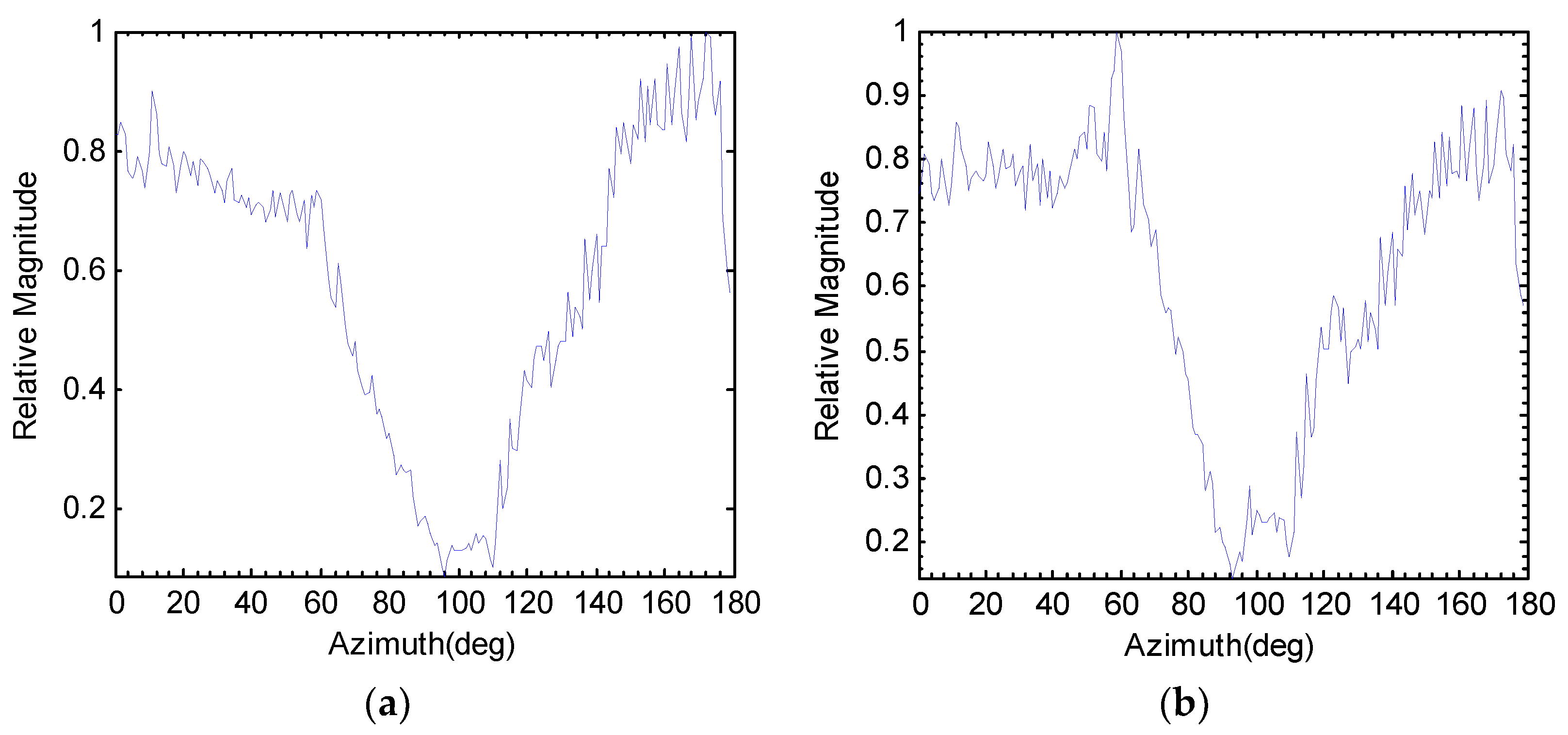
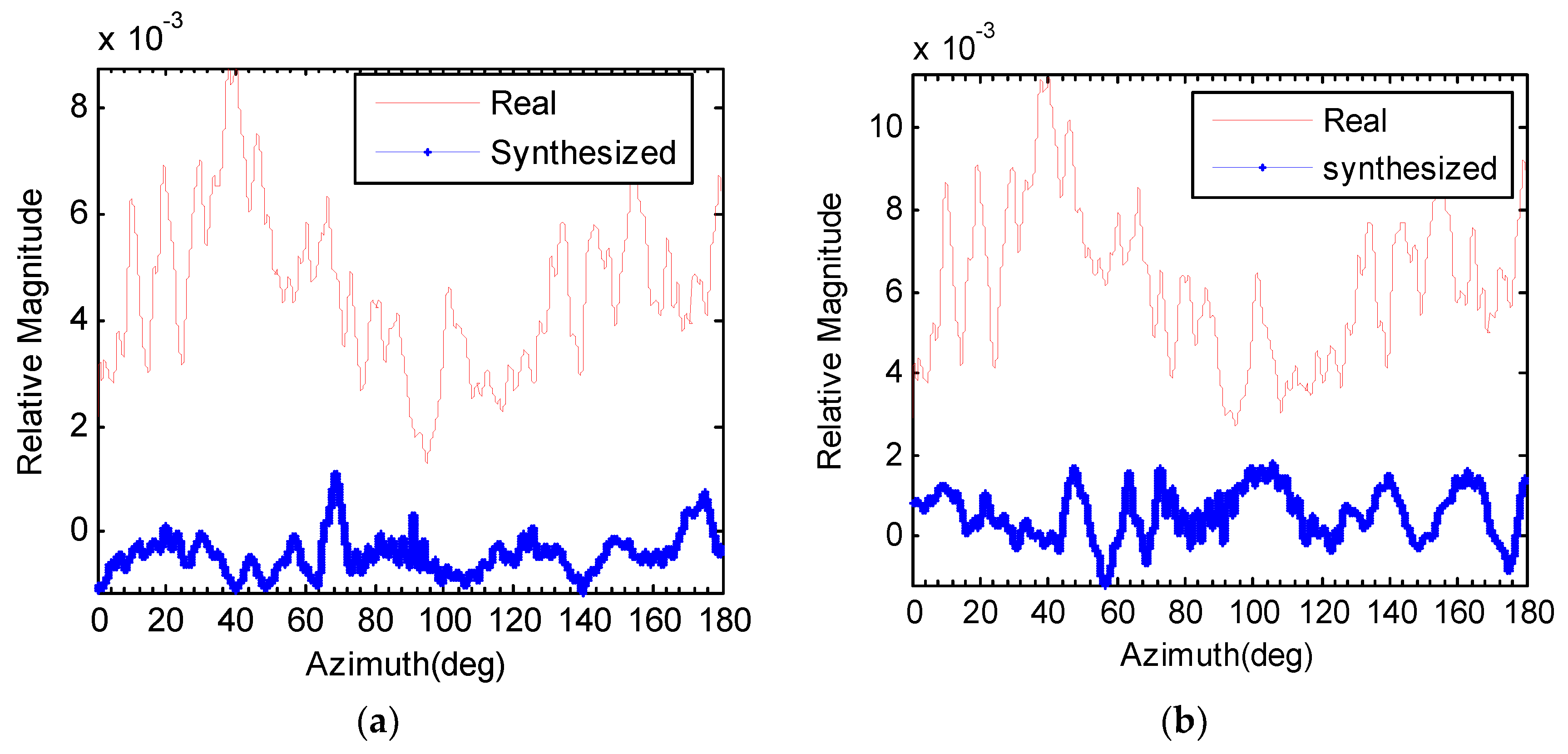
For further comparison, Figure 21 is the difference in the fluctuation intensity between the two different carrier frequency echoes. Figure 20a compares the difference in the fluctuation intensity from Figure 18, and Figure 21b compares the difference in the STD from Figure 19. In Figure 21, we can see that the fluctuation intensity and its STD of the real target echo change notably when the carrier frequency changes, but the fluctuation intensity and its STD do not present notable differences when the carrier frequency changes. Then, the real target echo and synthetic echo could be discriminated by the difference in those two features. The experimental results demonstrate the feasibility of the method that is proposed.
6. Discussion and Conclusions
In this study, the characteristics of echo envelope fluctuation intensity were studied, two features of which were characterized. The data processing results of the simulation and scaled benchmark tests are consistent. The echo envelope fluctuation intensity and its STD features strongly depend on the carrier frequency: when the carrier frequency increases, the echo envelope fluctuation intensity increases correspondingly. The magnitude of the echo fluctuation intensity and its STD vary with azimuth, which is minimum on the beam, and maximum on the keel-line. This is because the time difference between the echo highlights in the keel-line is greater than that in the beam direction, causing a larger magnitude fluctuation of the echo envelope. The magnitude of the fluctuation intensity changes as the pulse length changes—when the pulse length increases, the magnitude of the echo fluctuation intensity decreases. The fluctuation intensity and its STD could be used to characterize the fluctuation in the echo envelope magnitude, but the sensitivity of the standard deviation of the fluctuation intensity is relatively low, compared to that of the fluctuation intensity, especially for a narrowband signal.
Based on these echo envelope fluctuation characteristics, we propose a novel method for discriminating between a real underwater target echo and synthetic echo. The feasibility of the method was verified through a sea experiment.
It should be noted that the waveform structure of the synthetic echo becomes more like the real target echo when the number of highlights simulated by the echo decoy increases. The performance of this proposed method for a more complex synthetic echo will be studied in further work.
Author Contributions
All authors contributed significantly to the work presented in this manuscript. Y.C. proposed the novel method and wrote the paper; B.J. and Z.W. conceived and designed the experiments; G.L. and S.L. contributed with valuable discussions and scientific advice.
Funding
This research was funded in part by the Foundation of Science and Technology on Underwater Test and Control Laboratory under grant no. 9140C260201130C26096, and the APC was funded by that too.
Acknowledgments
The authors are grateful to Jun Fan from Shanghai Jiao Tong University for the acoustic scattering program code based on the Planar Element Method that originally developed by Jun Fan.
Conflicts of Interest
The authors declare no conflict of interest.
References
- He, X.Y.; Jiang, X.Z.; Liu, J.Y. Submarine echo simulation based on echo highlight model. J. Unmanned Undersea Syst. 2001, 9, 15–18. [Google Scholar]
- Lin, W.; Liu, L.J.; Xu, Y. Simulation of Underwater target echo based on highlight model. Appl. Mech. Mater. 2014, 536–537, 39–42. [Google Scholar] [CrossRef]
- He, C.; Zhao, A.B.; Zhou, B.; Song, X.; Niu, F. Parameter measurement research of sonar echo highlights. J. Acoust. Soc. Am. 2014, 135, 2303. [Google Scholar] [CrossRef]
- Cerqueira, R.; Trocoli, T.; Neves, G.; Joyeux, S.; Albiez, J.; Oliveira, L. A novel GPU-Based sonar simulator for real-time applications. Comput. Graphics 2017, 68, 66–76. [Google Scholar] [CrossRef]
- Gokhan, I.; Ozgur, B.A. Three-dimensional underwater target tracking with acoustic sensor networks. IEEE Trans. Veh. Technol. 2011, 60, 3897–3906. [Google Scholar]
- Luo, J.H.; Han, Y.; Fan, L.Y. Underwater acoustic target tracking: A review. Sensors 2018, 13, 112. [Google Scholar] [CrossRef] [PubMed]
- Seo, Y.; On, B.; Im, S.; Shim, T.; Seo, I. Underwater Cylindrical Object Detection Using the Spectral Features of Active Sonar Signals with Logistic Regression Models. Appl. Sci. 2018, 8, 116. [Google Scholar] [CrossRef]
- Meng, Q.X.; Yang, S.E. A wave structure based method for recognition of marine acoustic target signals. J. Acoust. Soc. Am. 2014, 137, 2242. [Google Scholar] [CrossRef]
- Fan, J. Study on Echo Characteristics of Underwater Complex Targets. Ph.D. Thesis, Shanghai Jiaotong University, Shanghai, China, 2001; p. 16. [Google Scholar]
- Jia, H.J.; Li, X.K.; Meng, X.X. Rigid and elastic acoustic scattering signal separation for underwater target. J. Acoust. Soc. Am. 2017, 142, 653–665. [Google Scholar] [CrossRef] [PubMed]
- Yang, M.; Li, X.; Yang, Y.; Meng, X. Characteristic analysis of underwater acoustic scattering echoes in the wavelet transform domain. J. Mar. Sci. Appl. 2017, 16, 93–101. [Google Scholar] [CrossRef]
- Wu, Y.S.; Li, X.K.; Wang, Y. Extraction and classification of acoustic scattering from underwater target based on Wigner-Ville distribution. Appl. Acoust. 2018, 138, 52–59. [Google Scholar] [CrossRef]
- Xu, G.F.; Li, C.X.; Ding, S.Q. Study on extracting the information of elastic scattering wave. Ocean Technol. 2006, 25, 94–98. [Google Scholar]
- Tang, W.L. Highlight model of echoes from sonar targets. ACTA Acoust. 1994, 19, 92–100. [Google Scholar]
- Lou, S.C.; Chao, R.M.; Ko, S.; Lin, K.M.; Zhong, J.X. A simplified signal analysis algorithm for the development of a low cost underwater echo-sounder. Measurement 2011, 44, 1572–1581. [Google Scholar] [CrossRef]
- Wang, M.Z.; Huang, X.W.; Hao, C.Y. Model of an underwater target based on target echo highlight structure. J. Syst. Simul. 2003, 15, 21–25. [Google Scholar]
- Muller, M.W.; Au, W.W.; Nachtigall, P.E.; Allen, J.S., III; Breese, M. Phantom echo highlight amplitude and temporal difference resolutions of an echolocating dolphin, Tursiops truncates. J. Acoust. Soc. Am. 2007, 122, 2255–2262. [Google Scholar] [CrossRef] [PubMed]
- Dankiewicz, L.A.; Helweg, D.A.; Moore, P.W.; Zafran, J.M. Discrimination of amplitude-modulated synthetic echo trains by an echolocating bottlenose dolphin. J. Acoust. Soc. Am. 2002, 112, 1702–1708. [Google Scholar] [CrossRef] [PubMed] [Green Version]
- Chen, Y.F.; Li, G.J.; Wang, Z.S.; Zhang, M.W.; Jia, B. Statistical feature of underwater target echo highlight. Acta Phys. Sin. 2013, 62, 084302. [Google Scholar]
- Chen, Y.F.; Li, S.; Wang, Z.S.; Li, G.J.; Gao, F. Echo magnitude fluctuation feature of underwater target. J. Ship Mech. 2017, 21, 218–227. [Google Scholar]
- Chen, Y.F.; Jia, B.; Li, S.; Wang, Z.S.; Li, G.J. Discrimination of real underwater target echo and synthetic echo based on envelope modulation rate. J. Harbin Eng. Univ. 2016, 37, 1467–1472. [Google Scholar]
- Nell, C.W.; Gilroy, L.E. An Improved BASIS Model for the BeTSSi Submarine; DRDC Atlantic TR 2003-199; Defence R&D Canada: Ottawa, ON, Canada, November 2003.
- Fan, J.; Zhu, B.L.; Tang, W.L. Modified geometrical highlight model of echoes from non-rigid surface sonar target. Acta Acust. 2001, 26, 545–550. [Google Scholar]
- Fan, J.; Li, J.L.; Liu, T. Transition characteristics of echoes from complex shape targets in water. J. Shanghai Jiaotong Univ. 2002, 36, 161–164. [Google Scholar]
- Fan, J.; Tang, W.L.; Zhuo, L.K. Planar elements method for forecasting the echo characteristics from sonar targets. J. Ship Mech. 2012, 16, 171–180. [Google Scholar]
Figure 1.
(a) Intensity of echo envelope fluctuation after normalization, the frequency is 20–40 kHz and the pulse length is 1 ms; (b) STD of echo envelope fluctuation after normalization.
Figure 1.
(a) Intensity of echo envelope fluctuation after normalization, the frequency is 20–40 kHz and the pulse length is 1 ms; (b) STD of echo envelope fluctuation after normalization.

Figure 2.
(a) Intensity of echo envelope fluctuation after normalization, the frequency is 20–40 kHz and the pulse length is 3 ms; (b) STD of echo envelope fluctuation after normalization.
Figure 2.
(a) Intensity of echo envelope fluctuation after normalization, the frequency is 20–40 kHz and the pulse length is 3 ms; (b) STD of echo envelope fluctuation after normalization.

Figure 3.
(a) Fluctuation intensity comparison of echo envelopes with different frequencies; (b) STD comparison of echo envelope fluctuation intensity with different frequencies.
Figure 3.
(a) Fluctuation intensity comparison of echo envelopes with different frequencies; (b) STD comparison of echo envelope fluctuation intensity with different frequencies.
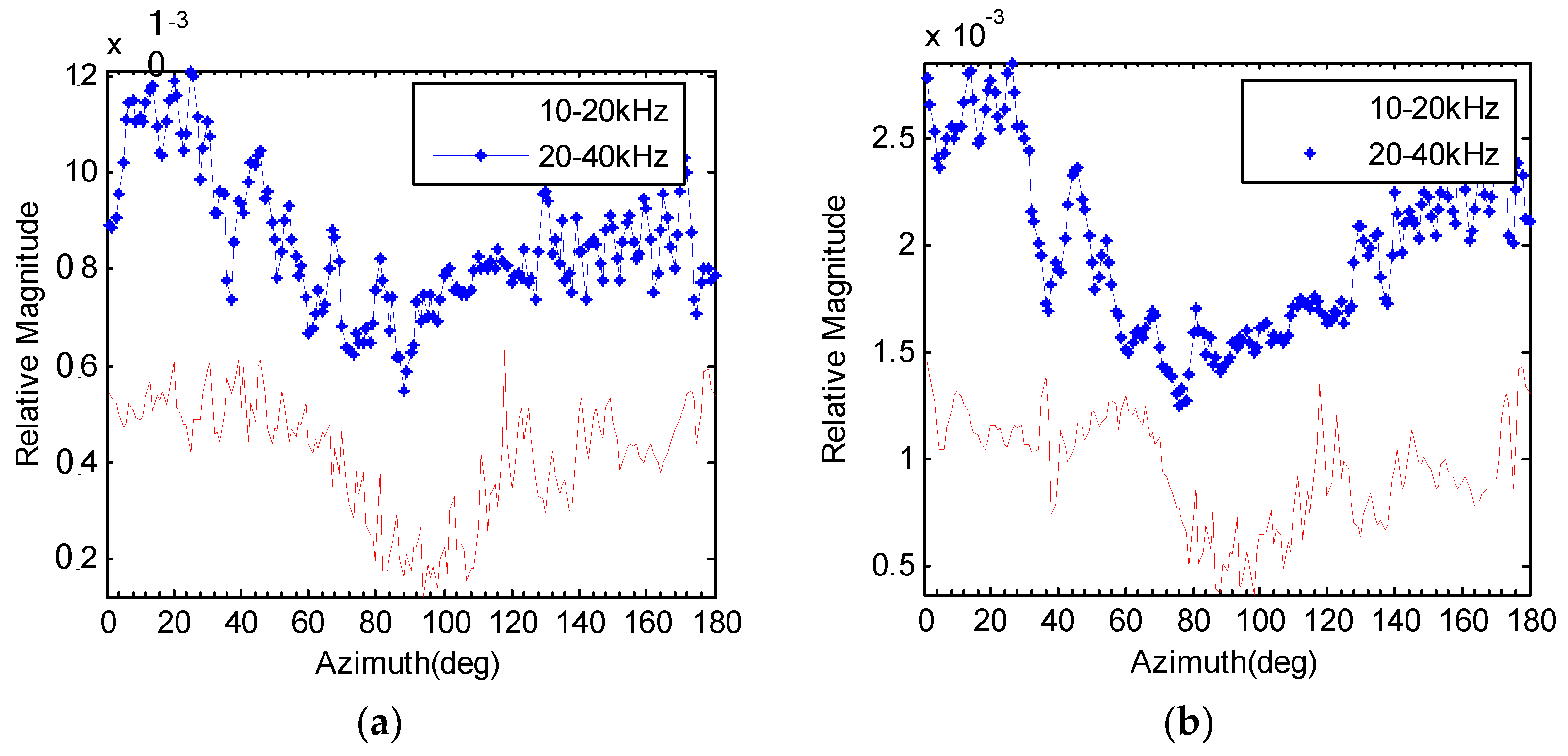
Figure 4.
(a) Fluctuation intensity comparison of a synthetic echo envelope with different frequencies; (b) STD comparison of synthetic echo envelope fluctuation intensity with different frequencies.
Figure 4.
(a) Fluctuation intensity comparison of a synthetic echo envelope with different frequencies; (b) STD comparison of synthetic echo envelope fluctuation intensity with different frequencies.

Figure 5.
Configuration of the benchmark sea experiment. (a) The schematic diagram of the experimental layout; (b) photo of the sea experiment; (c) photo of the rock that was tested.
Figure 5.
Configuration of the benchmark sea experiment. (a) The schematic diagram of the experimental layout; (b) photo of the sea experiment; (c) photo of the rock that was tested.

Figure 6.
(a) Echo envelope with LFM 20–40 kHz frequency; (b) gradient of the echo envelope from (a).
Figure 6.
(a) Echo envelope with LFM 20–40 kHz frequency; (b) gradient of the echo envelope from (a).
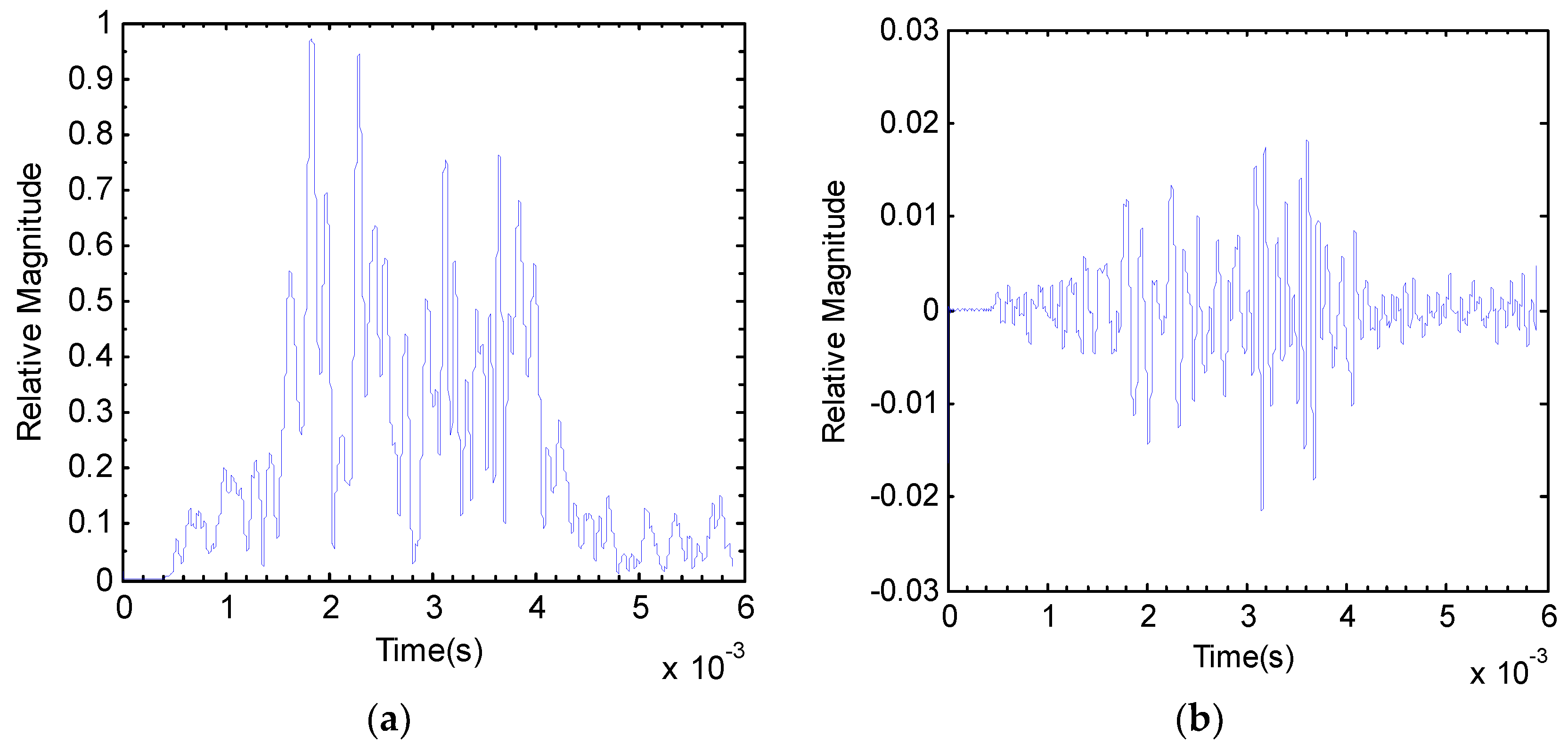
Figure 7.
(a) Echo envelope with LFM 40–80 kHz frequency; (b) gradient of the echo envelope from (a).
Figure 7.
(a) Echo envelope with LFM 40–80 kHz frequency; (b) gradient of the echo envelope from (a).
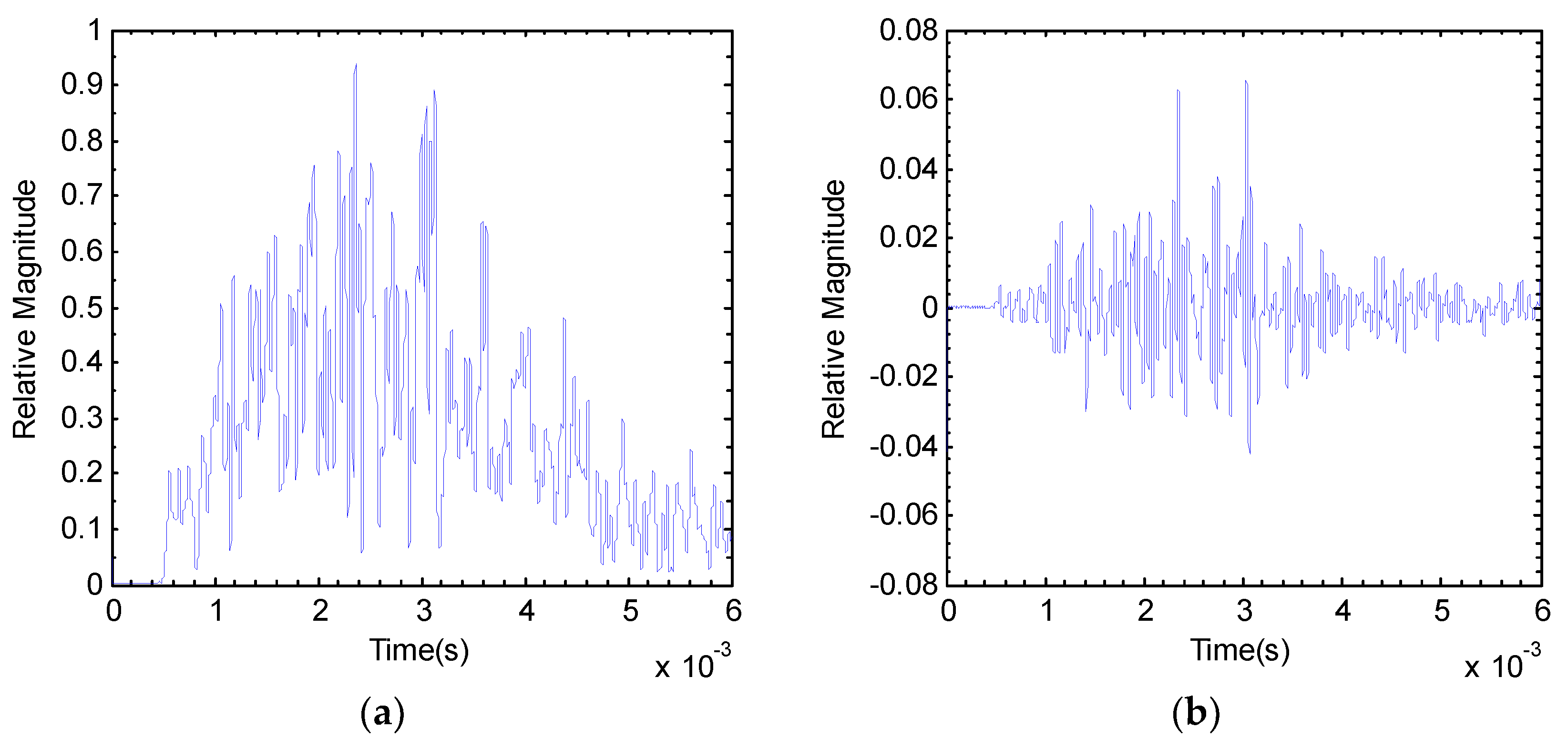
Figure 8.
Theoretical and tested echo envelope fluctuation intensity with the frequency of LFM 20–40 kHz. (a) The pulse length is 1 ms; (b) the pulse length is 3 ms.
Figure 8.
Theoretical and tested echo envelope fluctuation intensity with the frequency of LFM 20–40 kHz. (a) The pulse length is 1 ms; (b) the pulse length is 3 ms.

Figure 9.
(a) Fluctuation intensity comparison of the wideband echo envelope with different frequencies, the pulse length is 3 ms; (b) fluctuation intensity comparison of the CW echo envelope with different frequencies, the pulse length is 3 ms.
Figure 9.
(a) Fluctuation intensity comparison of the wideband echo envelope with different frequencies, the pulse length is 3 ms; (b) fluctuation intensity comparison of the CW echo envelope with different frequencies, the pulse length is 3 ms.
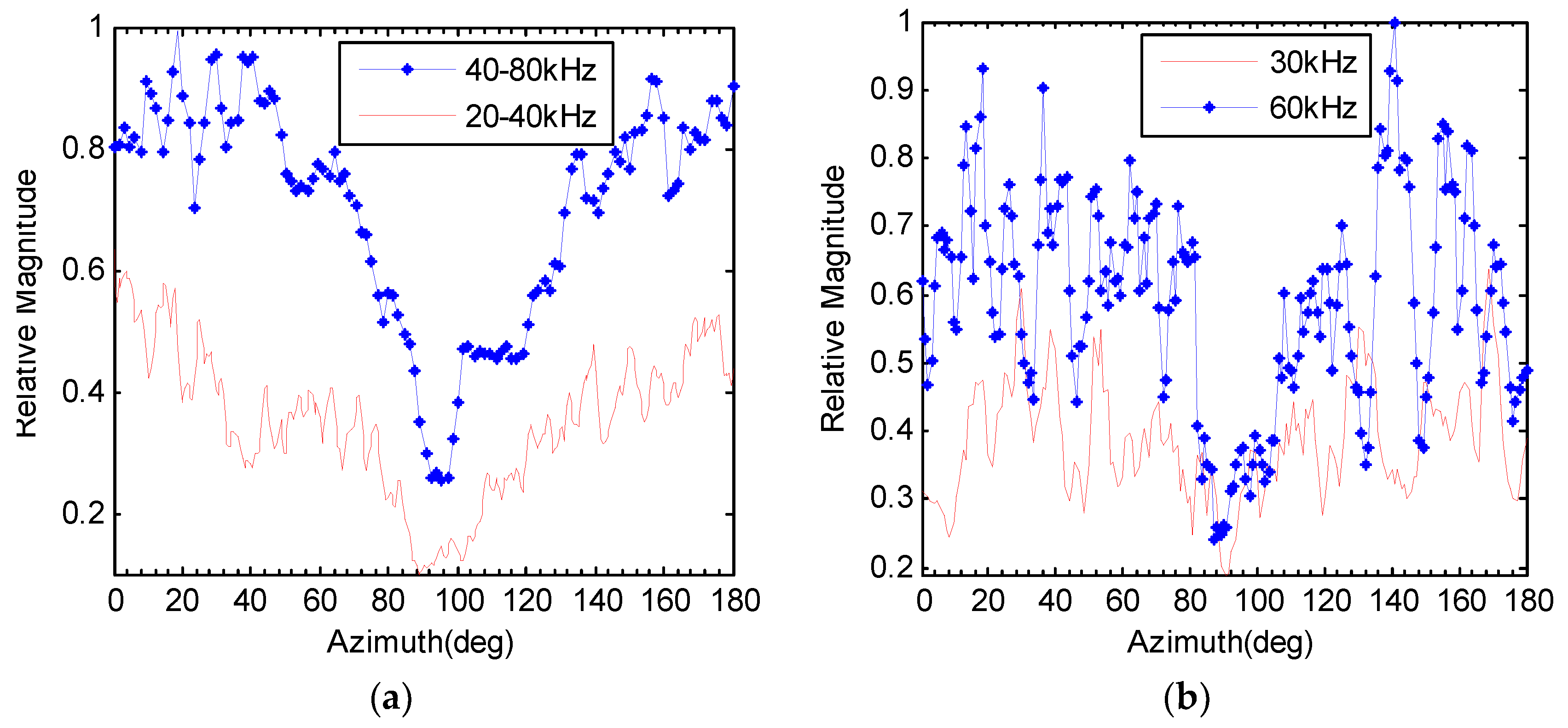
Figure 10.
(a) Fluctuation intensity of the CW echo envelope with different pulse lengths; (b) fluctuation intensity of the wideband echo envelope with different pulse lengths.
Figure 10.
(a) Fluctuation intensity of the CW echo envelope with different pulse lengths; (b) fluctuation intensity of the wideband echo envelope with different pulse lengths.

Figure 11.
STD of theoretical and tested echo envelope fluctuation intensity with the frequency of LFM 20–40 kHz. (a) The pulse length is 1 ms; (b) the pulse length is 3 ms.
Figure 11.
STD of theoretical and tested echo envelope fluctuation intensity with the frequency of LFM 20–40 kHz. (a) The pulse length is 1 ms; (b) the pulse length is 3 ms.

Figure 12.
STD of echo envelope fluctuation intensity with different frequencies, the pulse length is 3 ms. (a) STD comparison of wideband echo envelope fluctuation intensity with different frequencies; (b) STD comparison of CW echo envelope fluctuation intensity with different frequencies.
Figure 12.
STD of echo envelope fluctuation intensity with different frequencies, the pulse length is 3 ms. (a) STD comparison of wideband echo envelope fluctuation intensity with different frequencies; (b) STD comparison of CW echo envelope fluctuation intensity with different frequencies.

Figure 13.
(a) Fluctuation intensity comparison of the rock echo envelope with different frequencies; (b) STD comparison of the rock echo envelope fluctuation intensity with different frequencies.
Figure 13.
(a) Fluctuation intensity comparison of the rock echo envelope with different frequencies; (b) STD comparison of the rock echo envelope fluctuation intensity with different frequencies.
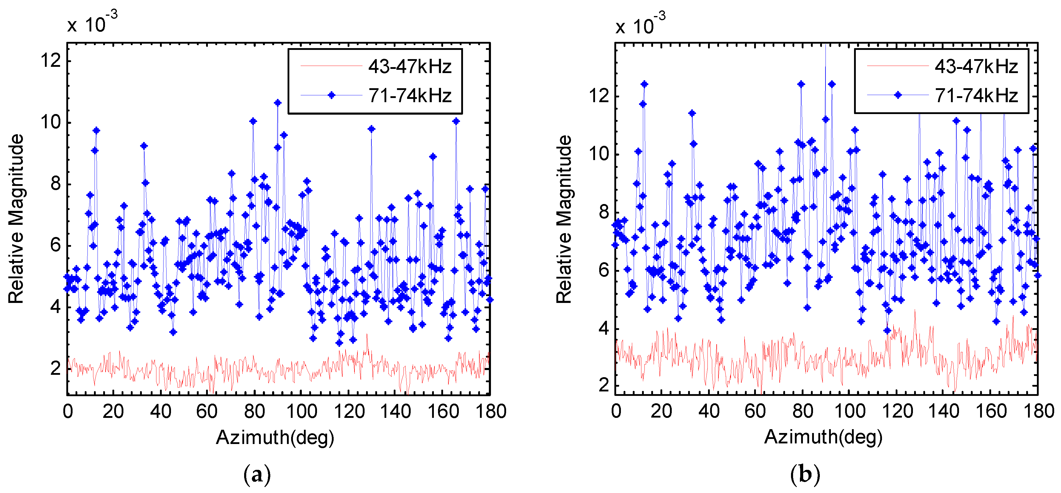
Figure 14.
Procedure for discriminating a real underwater target echo from a synthetic echo.

Figure 15.
Configuration of the synthetic echo test.
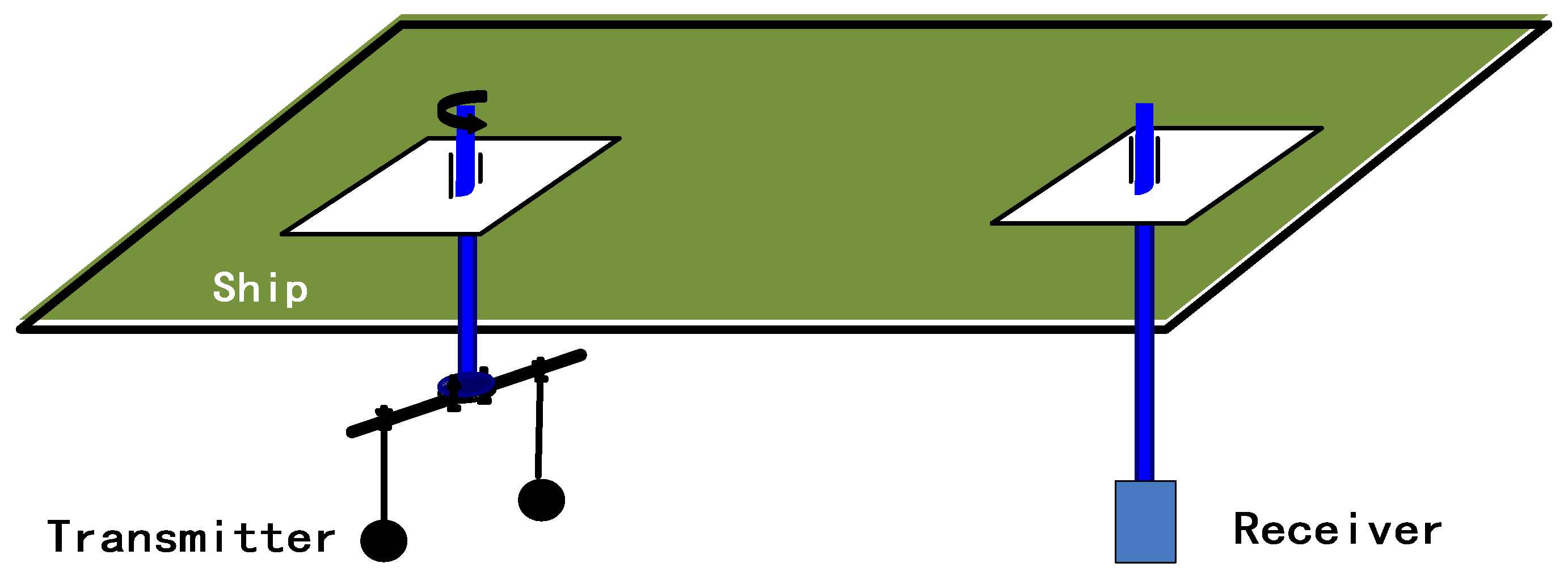
Figure 16.
(a) Synthetic echo envelope with LFM 20–40 kHz frequency; (b) gradient of the synthetic echo envelope from (a).
Figure 16.
(a) Synthetic echo envelope with LFM 20–40 kHz frequency; (b) gradient of the synthetic echo envelope from (a).
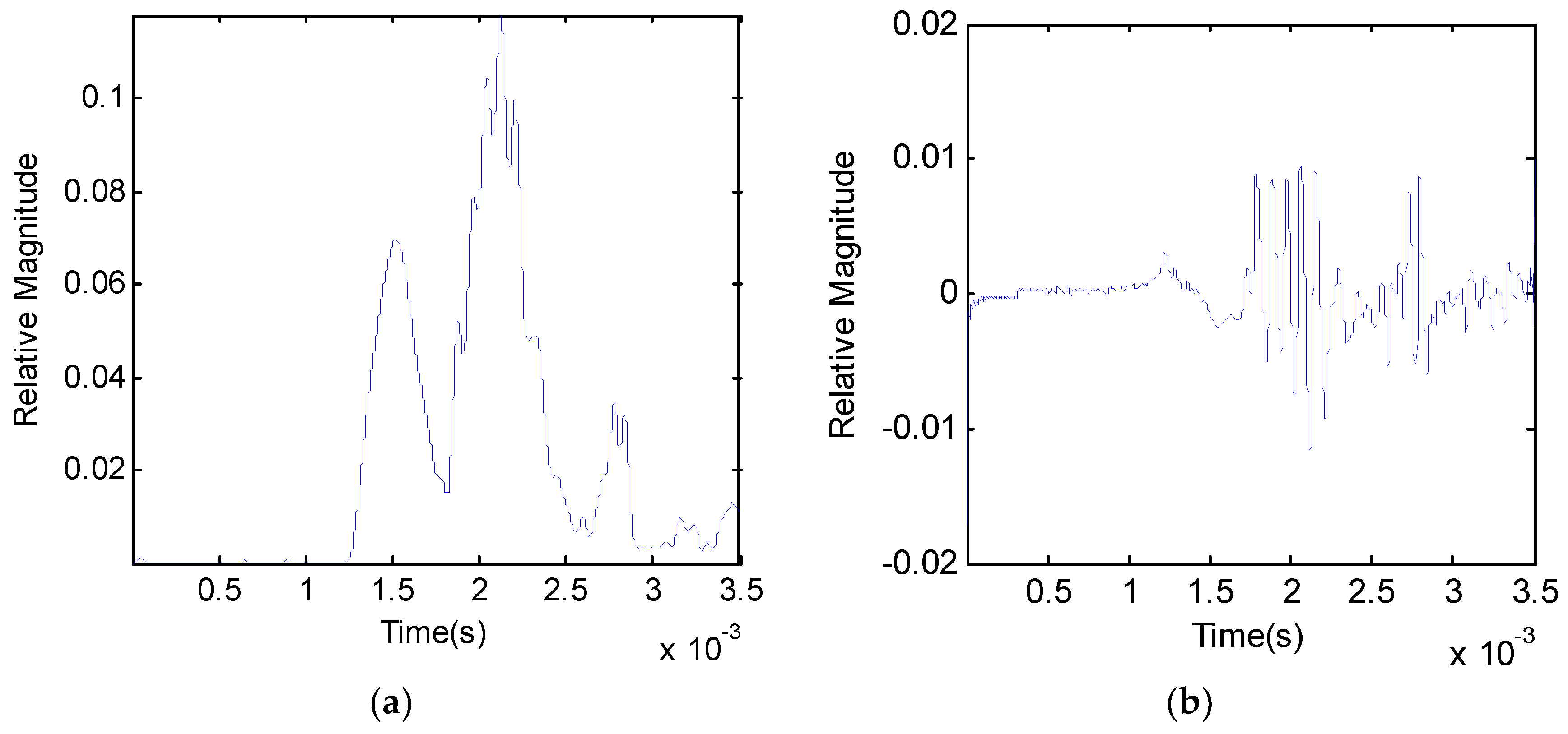
Figure 17.
(a) A synthetic echo envelope with LFM 40–80 kHz frequency; (b) gradient of the synthetic echo envelope from (a).
Figure 17.
(a) A synthetic echo envelope with LFM 40–80 kHz frequency; (b) gradient of the synthetic echo envelope from (a).
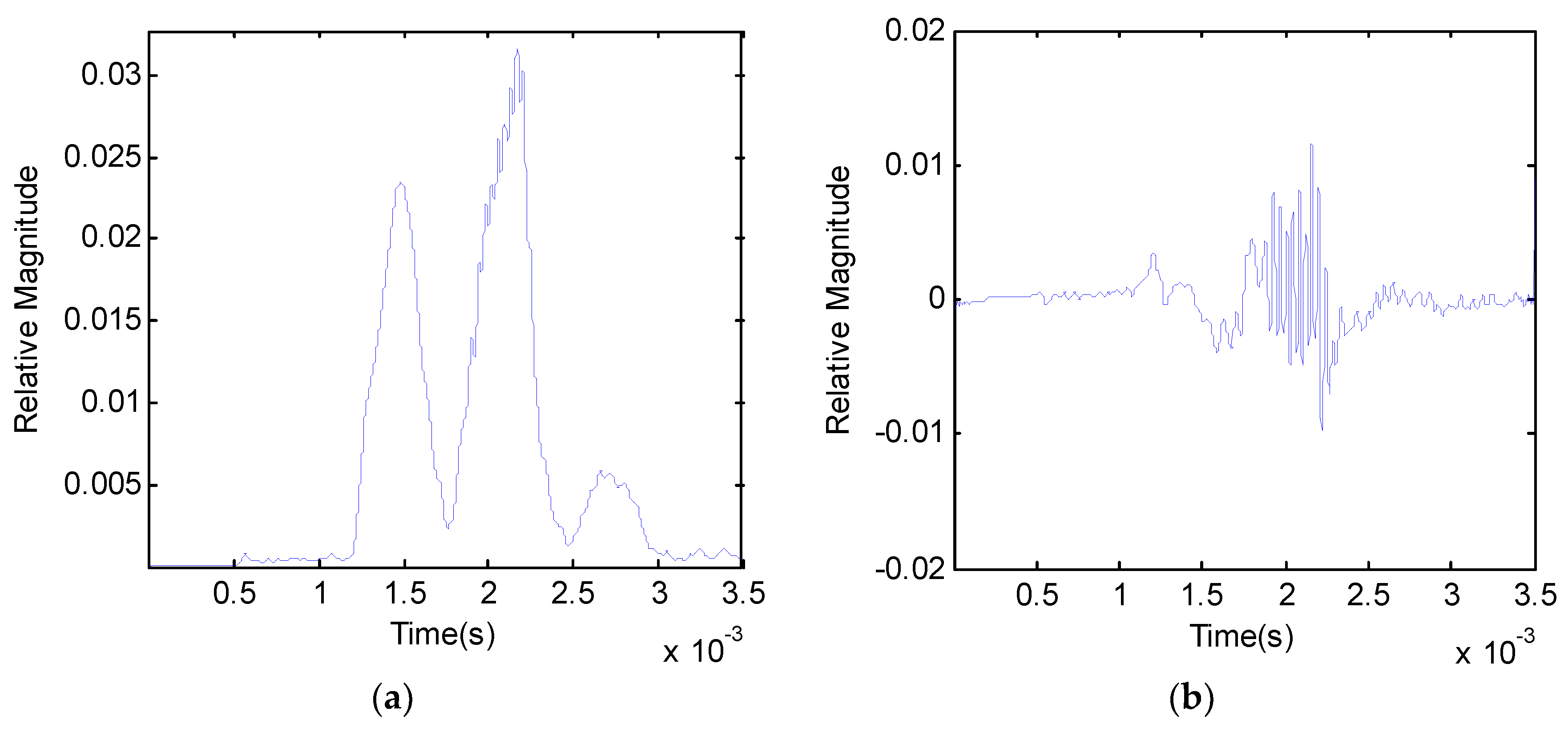
Figure 18.
(a) Fluctuation intensity comparison of the real target wideband echo envelope with different frequencies, the pulse length is 1 ms; (b) fluctuation intensity comparison of the synthetic wideband echo envelope with different frequencies, the pulse length is 1 ms.
Figure 18.
(a) Fluctuation intensity comparison of the real target wideband echo envelope with different frequencies, the pulse length is 1 ms; (b) fluctuation intensity comparison of the synthetic wideband echo envelope with different frequencies, the pulse length is 1 ms.

Figure 19.
(a) STD comparison of the real target wideband echo envelope with different frequencies, the pulse length is 1 ms; (b) STD comparison of the synthetic wideband echo envelope with different frequencies, the pulse length is 1 ms.
Figure 19.
(a) STD comparison of the real target wideband echo envelope with different frequencies, the pulse length is 1 ms; (b) STD comparison of the synthetic wideband echo envelope with different frequencies, the pulse length is 1 ms.
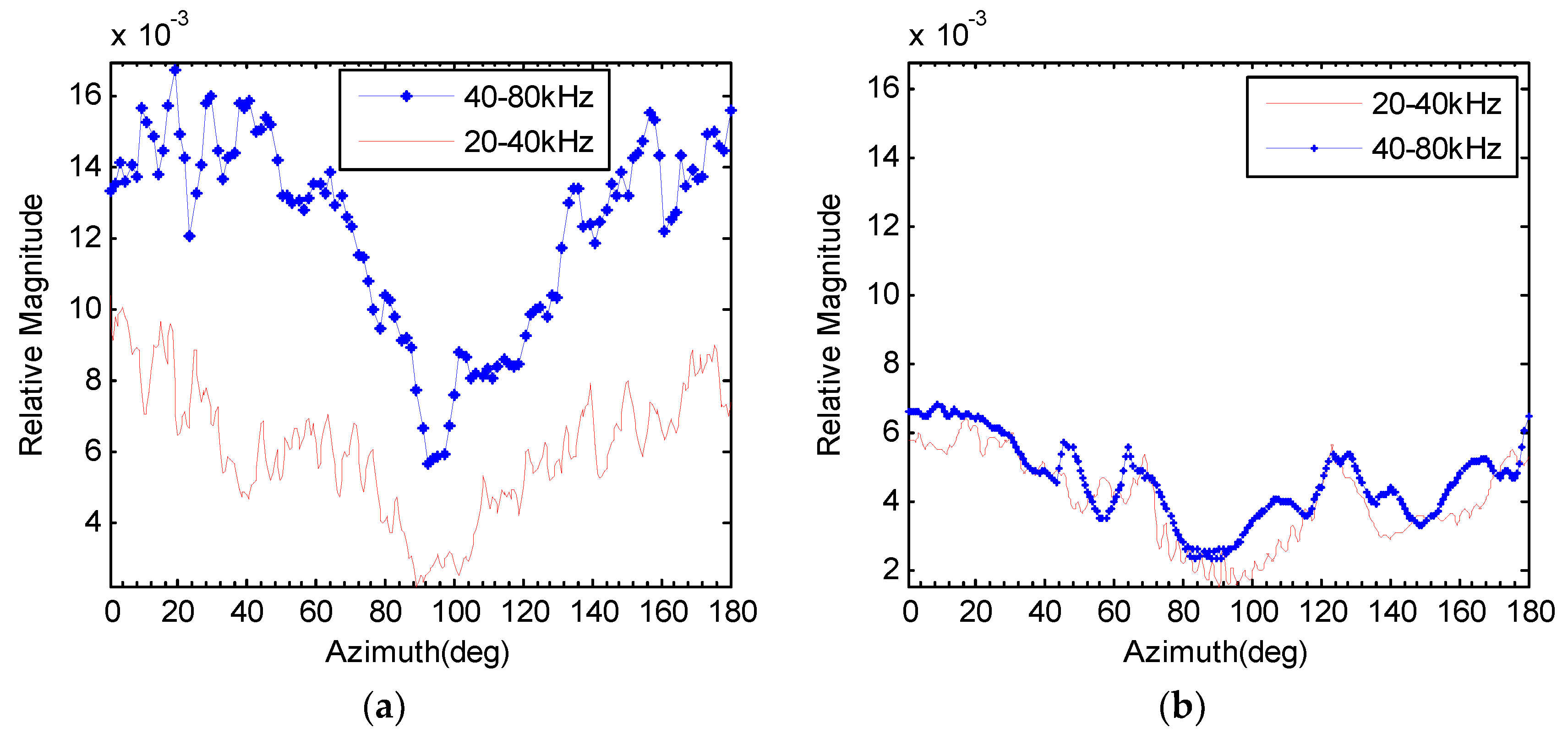
Figure 20.
(a) Fluctuation intensity comparison of the real target wideband echo envelope with different frequencies, the pulse length is 3 ms; (b) fluctuation intensity comparison of the synthetic wideband echo envelope with different frequencies, the pulse length is 3 ms.
Figure 20.
(a) Fluctuation intensity comparison of the real target wideband echo envelope with different frequencies, the pulse length is 3 ms; (b) fluctuation intensity comparison of the synthetic wideband echo envelope with different frequencies, the pulse length is 3 ms.
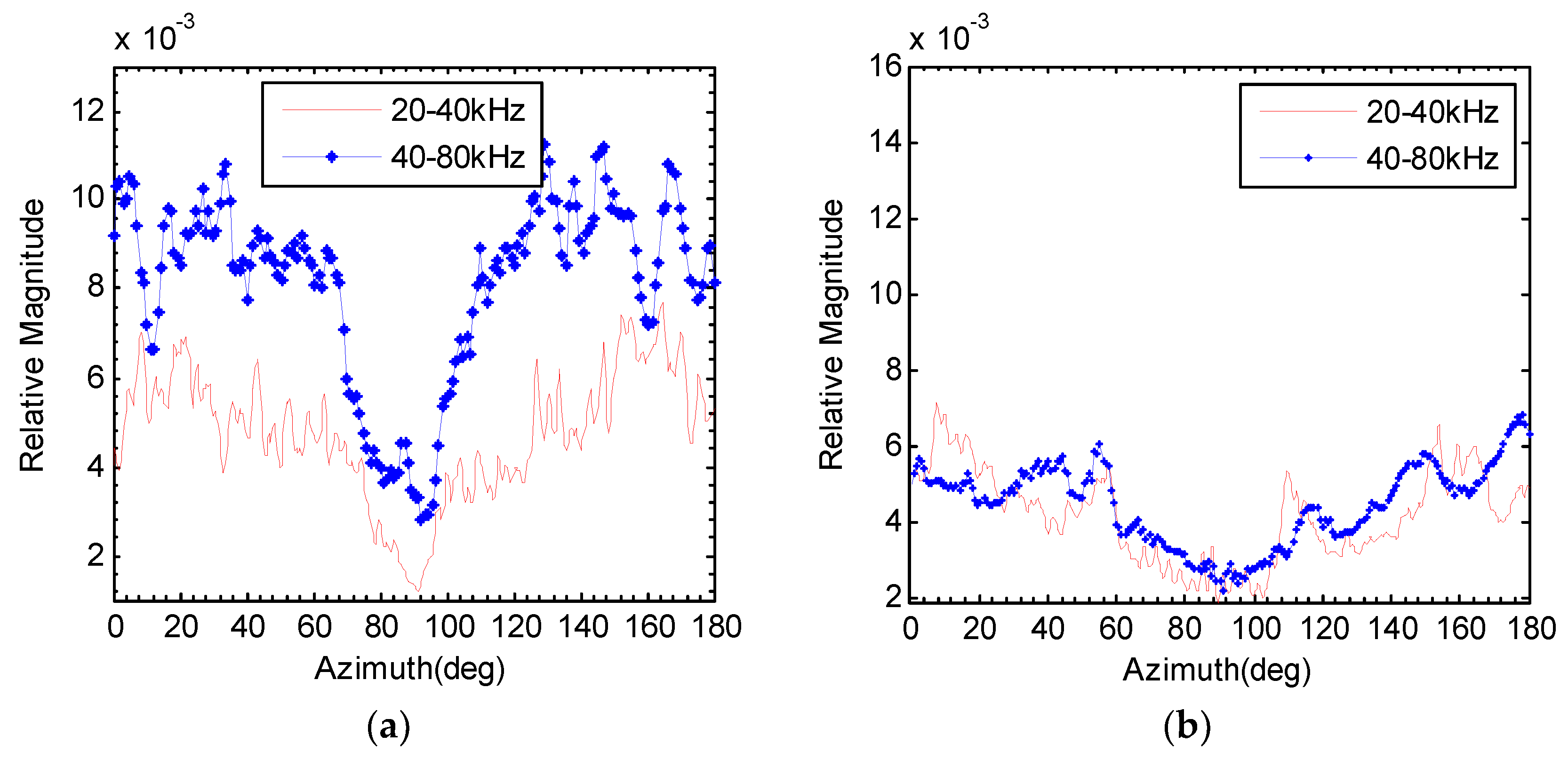
Figure 21.
(a) Fluctuation intensity difference comparison of Figure 18; (b) STD difference comparison of Figure 19.


Table 1.
Parameters of the incident signal.
| Signal Form | Frequency | Pulse Length | Target |
|---|---|---|---|
| CW | 30 kHz, 60 kHz | 1 ms, 3 ms, 10 ms | Benchmark model |
| LFM | 20–40 kHz, 40–80 kHz | 1 ms, 3 ms, 10 ms | Benchmark model |
| 43–47 kHz | 1 ms | Rock | |
| 71–74 kHz | 1 ms | Rock |
© 2018 by the authors. Licensee MDPI, Basel, Switzerland. This article is an open access article distributed under the terms and conditions of the Creative Commons Attribution (CC BY) license (http://creativecommons.org/licenses/by/4.0/).
Share and Cite
MDPI and ACS Style
Chen, Y.; Li, S.; Jia, B.; Li, G.; Wang, Z. Feature of Echo Envelope Fluctuation and Its Application in the Discrimination of Underwater Real Echo and Synthetic Echo. Appl. Sci. 2018, 8, 1329. https://doi.org/10.3390/app8081329
AMA Style
Chen Y, Li S, Jia B, Li G, Wang Z. Feature of Echo Envelope Fluctuation and Its Application in the Discrimination of Underwater Real Echo and Synthetic Echo. Applied Sciences. 2018; 8(8):1329. https://doi.org/10.3390/app8081329
Chicago/Turabian StyleChen, Yunfei, Sheng Li, Bing Jia, Guijuan Li, and Zhenshan Wang. 2018. "Feature of Echo Envelope Fluctuation and Its Application in the Discrimination of Underwater Real Echo and Synthetic Echo" Applied Sciences 8, no. 8: 1329. https://doi.org/10.3390/app8081329
Note that from the first issue of 2016, this journal uses article numbers instead of page numbers. See further details here.