Signal Pattern Recognition Based on Fractal Features and Machine Learning

Abstract
1. Introduction
2. Related Work
3. Fractal Dimension
3.1. Fractal Box Dimension
3.2. Katz Fractal Dimension
3.3. Higuchi Fractal Dimension
3.4. Petrosian Fractal Dimension
3.5. Sevcik Fractal Dimension
4. Classifier Algorithm
4.1. BP Neural Network
| Algorithm: BP Neural Network Classifier |
| Input: training dataset, testing dataset Output: classification result (label out) 1. Network initialization 2. Calculate the output of the network 3. Adjust the neurons’ weight in the network 4. Achieve the minimum value of the objective function 5. Output the classification result |
4.2. Grey Relational Analysis
| Algorithm: Grey Relational Analysis |
| Input: training dataset, testing dataset Output: classification result (label_out) 1. Determining the comparative sequence 2. For i = 1 to K Calculate the correlation degree End 3. = max() 4. Label out = find () 5. End |
4.3. K-Nearest Neighbor
| Algorithm: KNN Classifier |
| Input: training dataset, testing dataset Output: classification result (label out) 1. Calculate the weight of characteristic: 2. Calculate the vector space model of the training sample and the sample to be tested: 3. The distance of samples: 4. For i = 1 to K Calculate the weight of characteristic item: 5. = max() 6. Label out = find () 7. End |
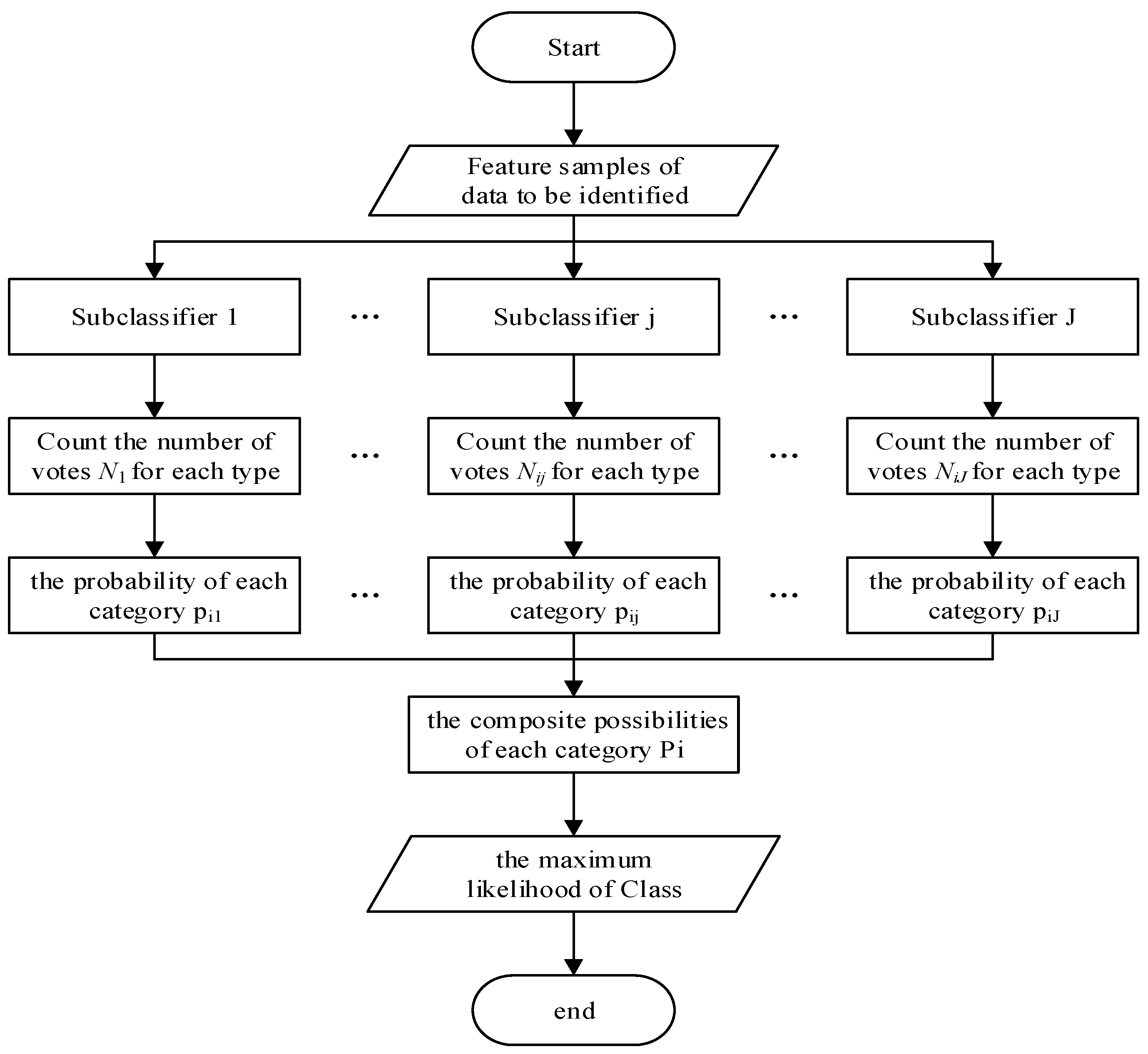
4.4. Random Forest
| Algorithm: Random Forest Classifier |
| Input: training dataset, testing dataset Output: classification result (label out) 1. Training J random forest classifiers 2. For i = 1 to J Calculate each probability of every classifier : End 3. Use Dempster–Shaferevidence theory to calculate each result probability of every classifier 4. = max() 5. Label out = find () 6. End |
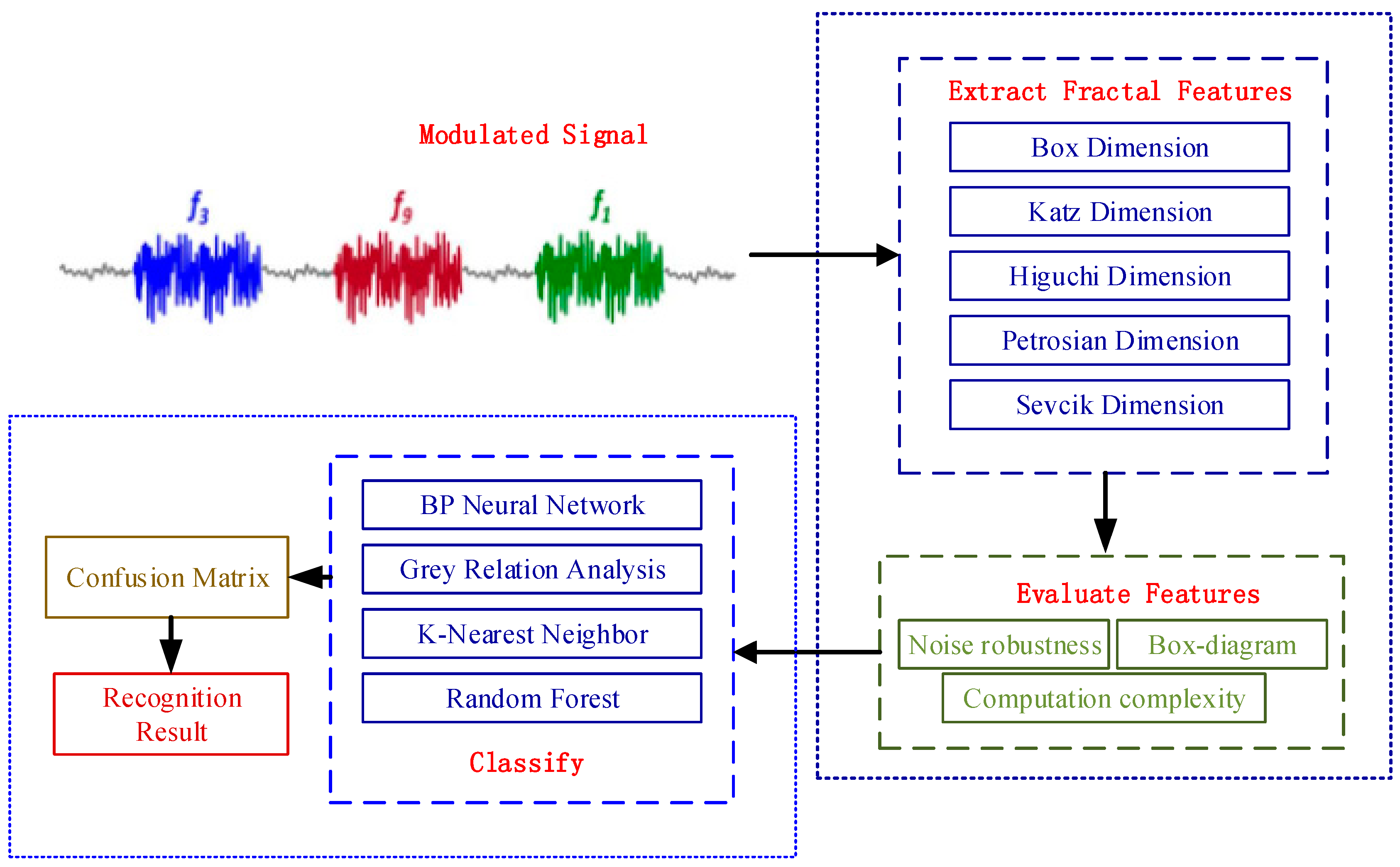
5. Simulation Results
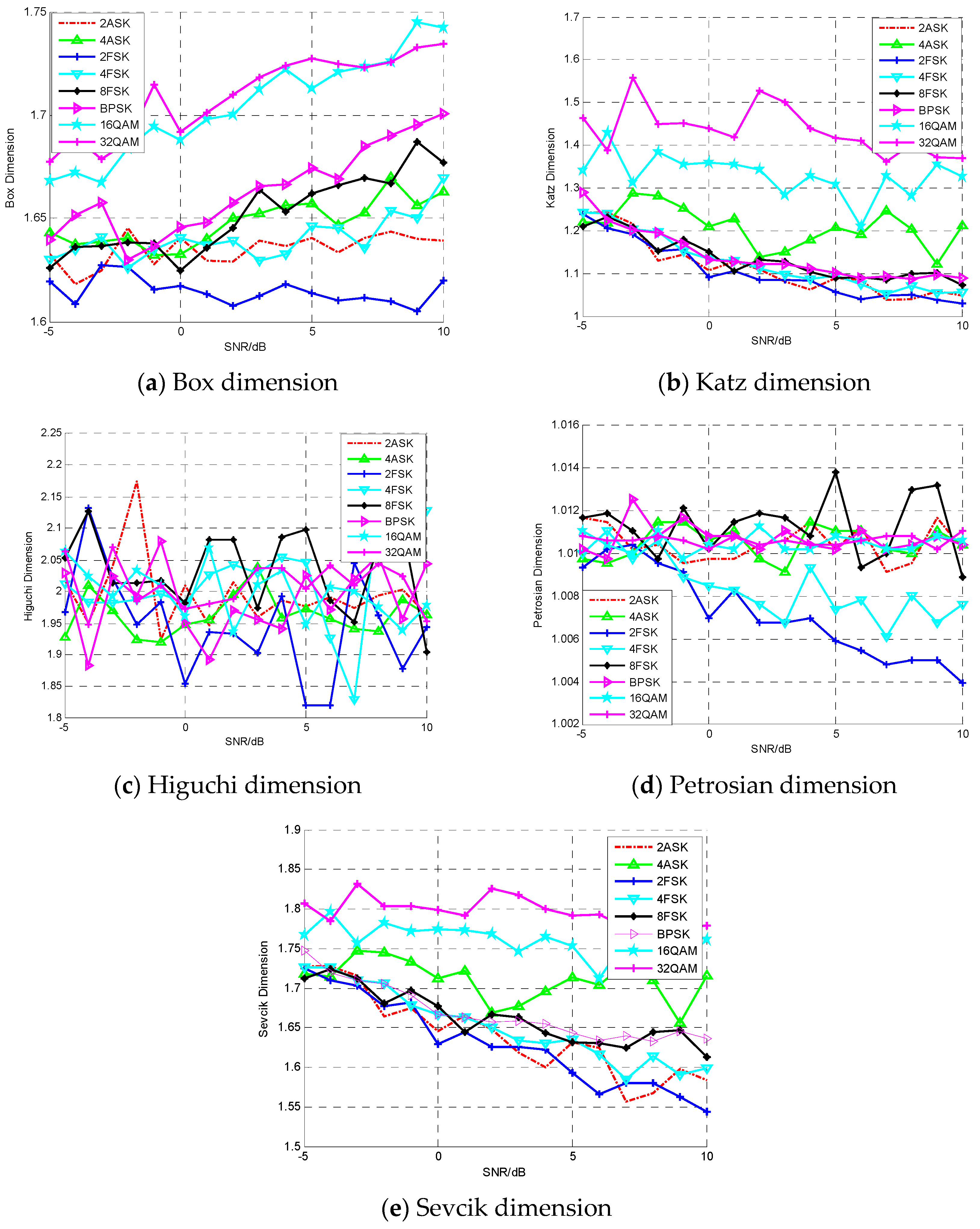
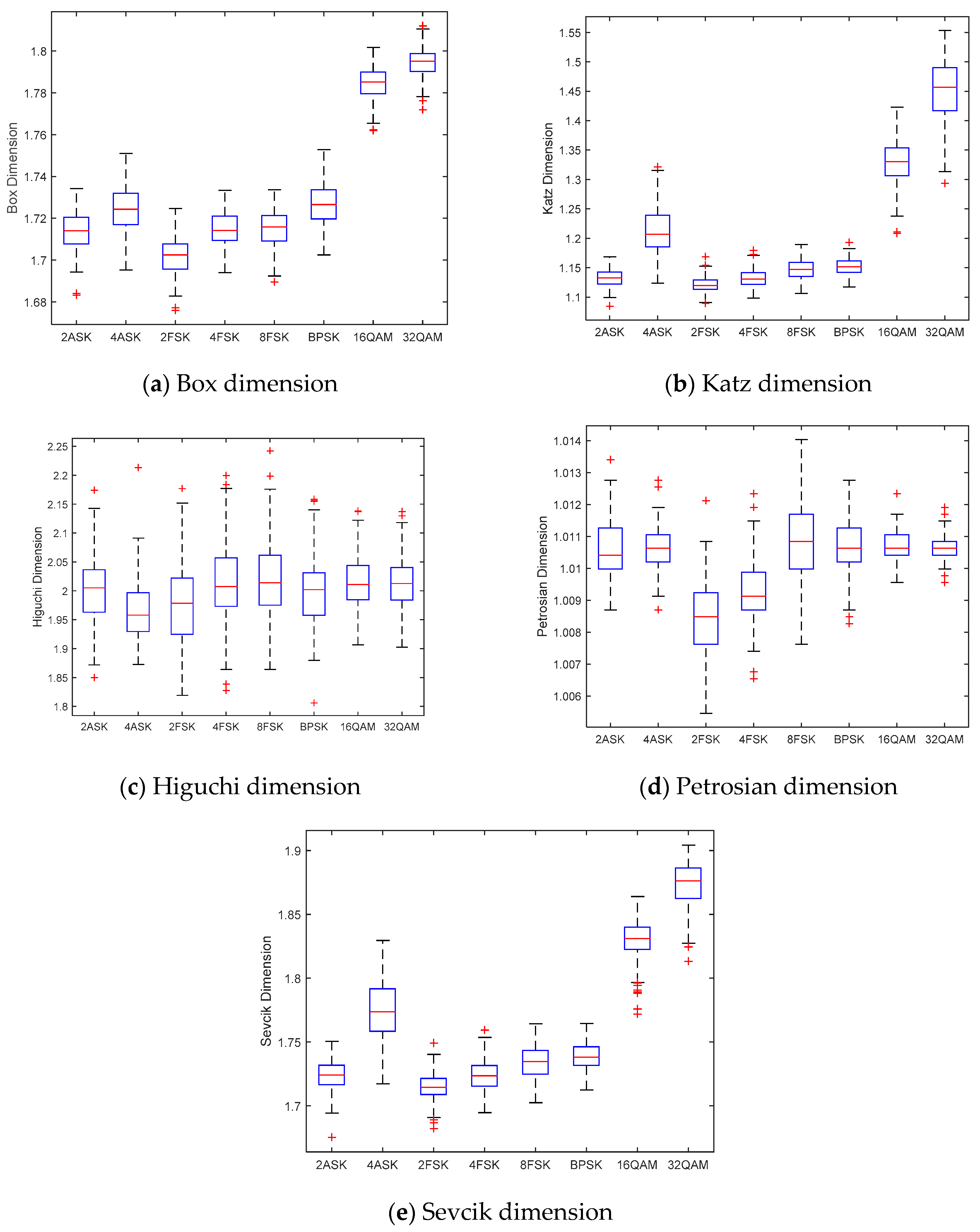
5.1. Simulation Analysis of Fractal Features
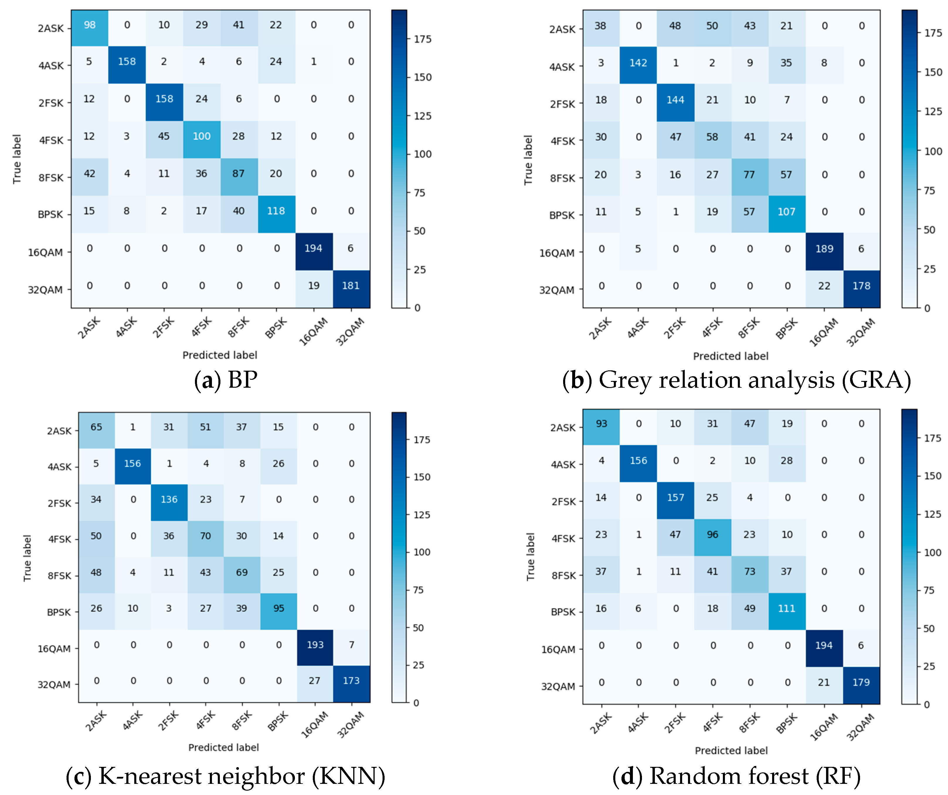
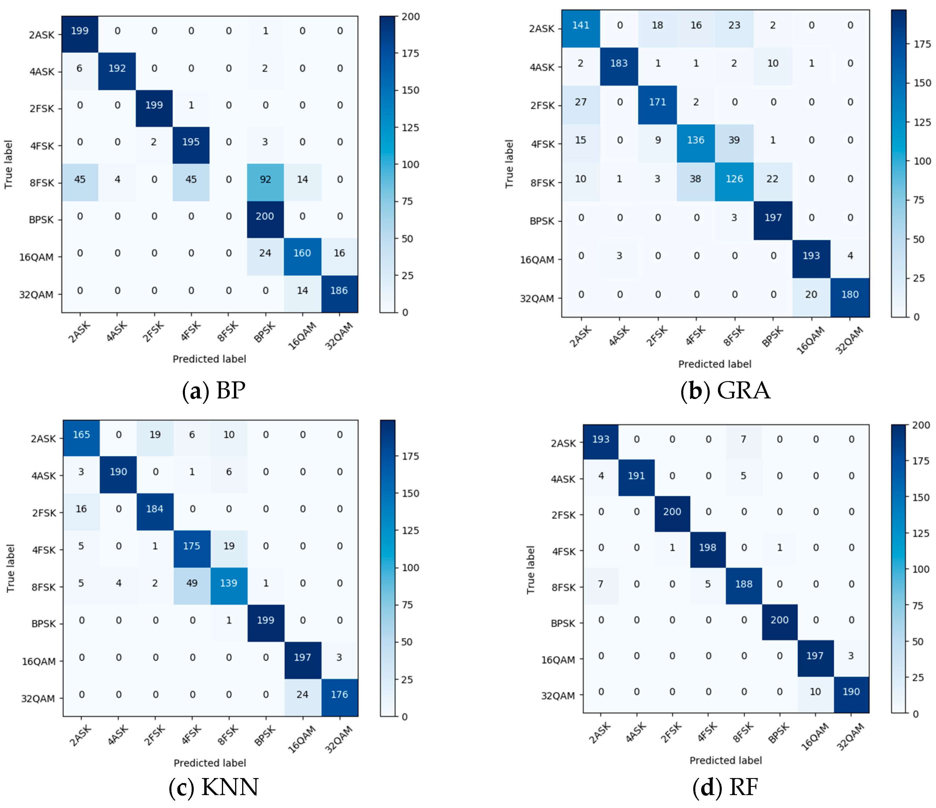
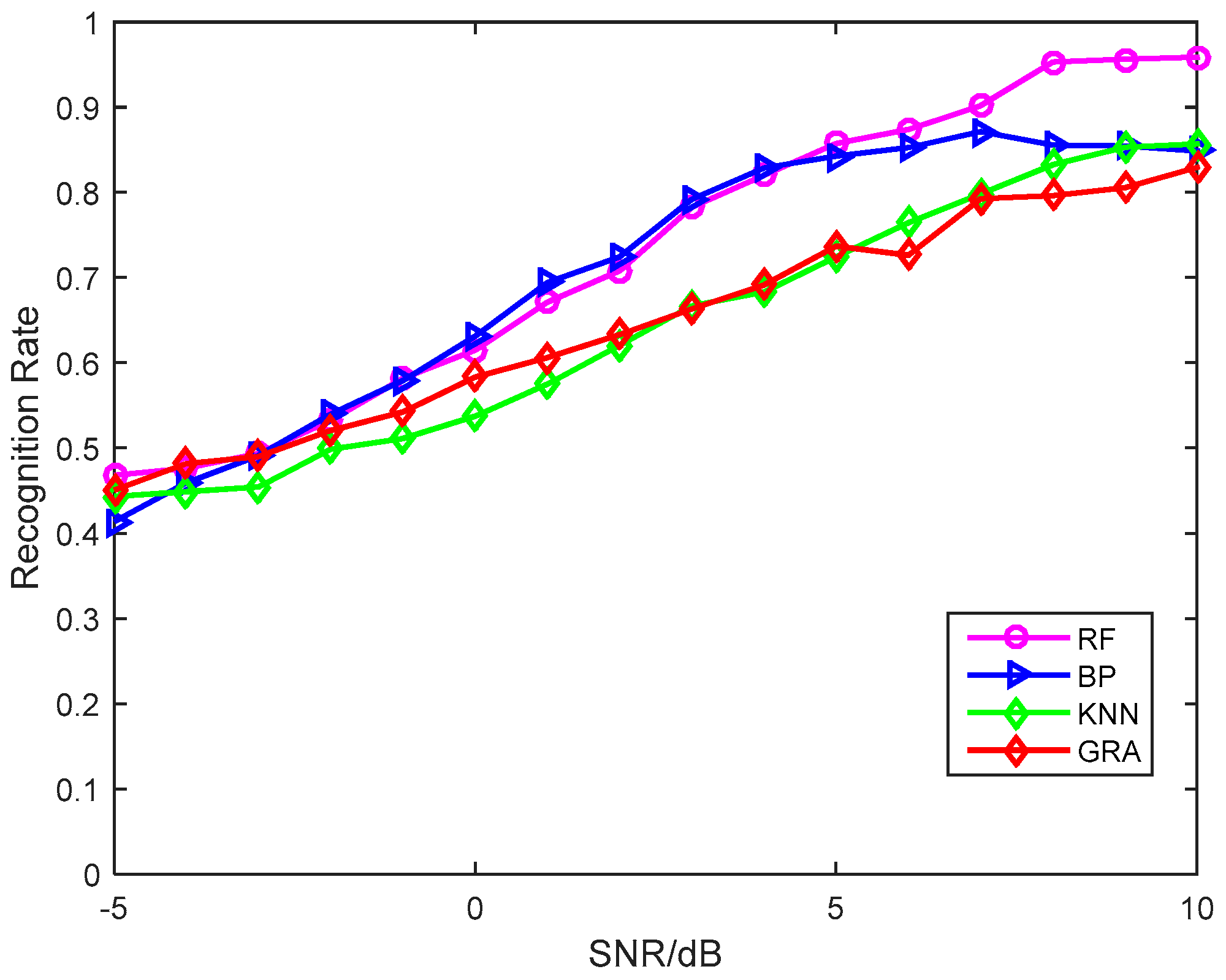
5.2. Classification Results
6. Conclusions
Funding
Conflicts of Interest
References
- Liu, K.; Zhang, X.; Chen, Y.Q. Extraction of Coal and Gangue Geometric Features with Multifractal Detrending Fluctuation Analysis. Appl. Sci. 2018, 8, 463. [Google Scholar] [CrossRef]
- Dahap, B.I.; Liao, H.S. Advanced algorithm for automatic modulation recognition for analogue & digital signals. In Proceedings of the International Conference on Computing, Control, Networking, Electronics and Embedded Systems Engineering, Khartoum, Sudan, 7–9 September 2015; pp. 32–36. [Google Scholar]
- Shen, Y.; Liu, X.; Yuan, X. Fractal Dimension of Irregular Region of Interest Application to Corn Phenology Characterization. IEEE J. Sel. Top. Appl. Earth Obs. Remote Sens. 2017, 10, 1402–1412. [Google Scholar] [CrossRef]
- Zhang, J.; Wang, X.; Yang, X. A method of constellation blind detection for spectrum efficiency enhancement. In Proceedings of the International Conference on Advanced Communication Technology, Pyeongchang, Korea, 31 January–3 February 2016. [Google Scholar]
- Wei, D.; Wei, J. A MapReduce Implementation of C4.5 Decision Tree Algorithm. Int. J. Database Theory Appl. 2014, 7, 49–60. [Google Scholar]
- Jiang, L.B.; Liu, Z.Z.; Wen, D.G. A New Recognition Algorithm of Digital Modulation Signals. Microelectron. Comput. 2013, 44, 112–123. [Google Scholar]
- Mehmood, R.M.; Lee, H.J. Emotion classification of EEG brain signal using SVM and KNN. In Proceedings of the IEEE International Conference on Multimedia & Expo Workshops, Turin, Italy, 29 June–3 July 2015; pp. 1–5. [Google Scholar]
- Jia, Y.U.; Chen, Y. Digital modulation recognition method based on BP neural network. Transducer Microsyst. Technol. 2012, 5, 7. [Google Scholar]
- Gharehbaghi, A.; Lindén, M. A Deep Machine Learning Method for Classifying Cyclic Time Series of Biological Signals Using Time-Growing Neural Network. IEEE Trans. Neural Netw. Learn. Syst. 2017. [Google Scholar] [CrossRef] [PubMed]
- Shi, X.; Liu, Y. Modified Artificial Bee Colony Algorithm Optimizing BP Neural Network and Its Application in the Digital Modulation Recognition. J. Jiangnan Univ. 2015, 4, 4. [Google Scholar]
- Deng, J.L. Introduction to Grey system theory. J. Grey Syst. 1989, 1, 1–24. [Google Scholar]
- Wang, X.; Wang, J.K.; Liu, Z.G.; Wang, B.; Hu, X. Spectrum Sensing for Cognitive Networks Based on Dimensionality Reduction and Random Forest. Int. J. Signal Process. Image Process. 2014, 7, 443–452. [Google Scholar] [CrossRef]
- Wang, X.; Gao, Z.; Fang, Y.; Yuan, S.; Zhao, H.; Gong, W.; Qiu, M.; Liu, Q. A Signal Modulation Type Recognition Method Based on Kernel PCA and Random Forest in Cognitive Network. In Proceedings of the International Conference on Intelligent Computing, Taiyuan, China, 3–6 August 2014; pp. 522–528. [Google Scholar]
- Zhang, Z.; Li, Y.; Zhu, X.; Lin, Y. A Method for Modulation Recognition Based on Entropy Features and Random Forest. In Proceedings of the IEEE International Conference on Software Quality, Reliability and Security Companion, Prague, Czech Republic, 25–29 July 2017. [Google Scholar]
- Zhang, Y.D.; Chen, X.Q.; Zhan, T.M.; Jiao, Z.Q.; Sun, Y.; Chen, Z.M.; Yao, Y.; Fang, L.T.; Lv, Y.D.; Wang, S.H. Fractal Dimension Estimation for Developing Pathological Brain Detection System Based on Minkowski-Bouligand Method. IEEE Access 2016, 4, 5937–5947. [Google Scholar] [CrossRef]
- Sanchez, J.P.; Alegria, O.C.; Rodriguez, M.V.; Abeyro, J.A.; Almaraz, J.R.; Gonzalez, A.D. Detection of ULF Geoma-gnetic Anomalies Associated to Seismic Activity Using EMD Method and Fractal Dimension Theory. IEEE Latin Am. Trans. 2017, 15, 197–205. [Google Scholar] [CrossRef]
- Zhao, N.; Yu, F.R.; Sun, H.; Li, M. Adaptive Power Allocation Schemes for Spectrum Sharing in Interference-Alignment-Based Cognitive Radio Networks. IEEE Trans. Veh. Technol. 2016, 65, 3700–3714. [Google Scholar] [CrossRef]
- Lin, Y.; Zhu, X.; Zheng, Z.; Dou, Z.; Zhou, R. The individual identification method of wireless device based on dimensionality reduction and machine learning. J. Supercomput. 2017, 74, 1–18. [Google Scholar] [CrossRef]
- Shi, C.; Dou, Z.; Lin, Y.; Li, W. Dynamic threshold-setting for RF-powered cognitive radio networks in non-Gaussian noise. Phys. Commun. 2018, 27, 99–105. [Google Scholar] [CrossRef]
- Yang, Z.; Deng, J.; Nallanathan, A. Moving Target Recognition Based on Transfer Learning and Three-Dimensional Over-Complete Dictionary. IEEE Sens. J. 2016, 16, 5671–5678. [Google Scholar] [CrossRef]
- Prieto, M.D.; Espinosa, A.G.; Ruiz, J.R.; Urresty, J.C.; Ortega, J.A. Feature Extraction of Demag-netization Faults in Permanent-Magnet Synchronous Motors Based on Box-Counting Fractal Dimension. IEEE Trans. Ind. Electron. 2011, 58, 1594–1605. [Google Scholar] [CrossRef]
- Zhou, J.T.; Xu, X.; Pan, S.J.; Tsang, I.W.; Qing, Z.; Goh, R.S.M. Transfer Hashing with Privileged Information. arXiv, 2016; arXiv:1605.04034. [Google Scholar]
- Vanthana, P.S.; Muthukumar, A. Iris authentication using Gray Level Co-occurrence Matrix and Hausdorff Dimension. In Proceedings of the International Conference on Computer Communication and Informatics, Coimbatore, India, 8–10 January 2015. [Google Scholar]
- Gui, Y. Hausdorff Dimension Spectrum of Self-Affine Carpets Indexed by Nonlinear Fibre-Coding. In Proceedings of the International Workshop on Chaos-Fractals Theories and Applications, Liaoning, China, 6–8 November 2009; pp. 382–386. [Google Scholar]
- Guariglia, E. Entropy and Fractal Antennas. Entropy 2016, 18, 84. [Google Scholar] [CrossRef]
- Sevcik, C. A Procedure to Estimate the Fractal Dimension of Waveforms. Complex. Int. 1998, 5, 1–19. [Google Scholar]
- Petrosian, A. Kolmogorov Complexity of Finite Sequences and Recognition of Different Preictal EEG Patterns. In Proceedings of the Computer-Based Medical Systems, Lubbock, TX, USA, 9–10 June 1995; pp. 212–217. [Google Scholar]
- Berry, M.V.; Lewis, Z.V.; Nye, J.F. On the Weierstrass-Mandelbrot fractal function. Proc. R. Soc. Lond. 1980, 370, 459–484. [Google Scholar] [CrossRef]
- Guariglia, E. Spectral Analysis of the Weierstrass-Mandelbrot Function. In Proceedings of the 2nd International Multidisciplinary Conference on Computer and Energy Science, Split, Croatia, 12–14 July 2017. [Google Scholar]
- Wang, H.; Li, J.; Guo, L.; Dou, Z.; Lin, Y.; Zhou, R. Fractal Complexity-based Feature Extra-ction Algorithm of Communication Signals. Fractals 2017, 25, 1740008. [Google Scholar] [CrossRef]
- Liu, S.; Pan, Z.; Cheng, X. A Novel Fast Fractal Image Compression Method based on Distance Clustering in High Dimensional Sphere Surface. Fractals 2017, 25, 1740004. [Google Scholar] [CrossRef]
- Lin, Y.; Wang, C.; Wang, J.; Dou, Z. A Novel Dynamic Spectrum Access Framework Based on Reinforcement Learning for Cognitive Radio Sensor Networks. Sensors 2016, 16, 1675. [Google Scholar] [CrossRef] [PubMed]
- Liu, S.; Pan, Z.; Fu, W.; Cheng, X. Fractal generation method based on asymptote family of generalized Mandelbrot set and its application. J. Nonlinear Sci. Appl. 2017, 10, 1148–1161. [Google Scholar] [CrossRef]
- Liu, S. Special issue on advanced fractal computing theorem and application. Fractals 2017, 25, 1740007. [Google Scholar]
- Liu, S.; Zhang, Z.; Qi, L.; Ma, M. A Fractal Image Encoding Method based on Statistical Loss used in Agricultural Image Compression. Multimed. Tools Appl. 2016, 75, 15525–15536. [Google Scholar] [CrossRef]


| Type | Box | Katz | Higuchi | Petrosian | Sevcik |
|---|---|---|---|---|---|
| SVar/ | 2.5 | 1.88 | 9 | 0.03 | 9.3 |
| Type | Box | Katz | Higuchi | Petrosian | Sevcik |
|---|---|---|---|---|---|
| Runtime/s | 1.92 | 1.66 | 82.199 | 2.83 | 1.26 |
© 2018 by the author. Licensee MDPI, Basel, Switzerland. This article is an open access article distributed under the terms and conditions of the Creative Commons Attribution (CC BY) license (http://creativecommons.org/licenses/by/4.0/).
Share and Cite
Shi, C.-T. Signal Pattern Recognition Based on Fractal Features and Machine Learning. Appl. Sci. 2018, 8, 1327. https://doi.org/10.3390/app8081327
Shi C-T. Signal Pattern Recognition Based on Fractal Features and Machine Learning. Applied Sciences. 2018; 8(8):1327. https://doi.org/10.3390/app8081327
Chicago/Turabian StyleShi, Chang-Ting. 2018. "Signal Pattern Recognition Based on Fractal Features and Machine Learning" Applied Sciences 8, no. 8: 1327. https://doi.org/10.3390/app8081327
APA StyleShi, C.-T. (2018). Signal Pattern Recognition Based on Fractal Features and Machine Learning. Applied Sciences, 8(8), 1327. https://doi.org/10.3390/app8081327