1. Introduction
One of the most interesting and widely studied properties of complex networks is community structure. While an exact definition of a
community is difficult to find, communities or clusters are often interpreted as groups of nodes that are more connected to each other than to the rest of the network. Because of this, nodes in a community “probably share common properties and/or play similar roles” within the network [
1]. Depending on the context,
community detection may also be referred to as
clustering or
graph partitioning.
Clustering is a very useful data exploratory machine learning tool that allows us to make better sense of heterogeneous data by grouping data with similar attributes based on some criteria. Popular graph partitioning methods such as the Girvan–Newman algorithm [
2], sparsest-cuts [
3], spectral partitioning [
4], and general conductance based methods (related to spectral methods via Cheeger’s inequality [
5]) may be viewed as solving an
edge-based resilience problem on a graph while simultaneously outputting the components resulting from the removal of the
critical edge set as the set of clusters. In contrast to these graph-theoretic edge-based resilience methods, in preliminary work [
6], we introduced a
node-based resilience clustering approach using
vertex attack tolerance (VAT) [
7,
8,
9,
10] with some unique applicability for noisy datasets. A node-based resilience measure by definition must express the relative size of a most critical set of target vertices whose removal, upon an attack, would be detrimental to the remaining network and attempt to quantify the amount of resulting damage [
10].
We are the first to establish a relationship between combinatorial measures of node-based resilience and graph-theoretic clustering. The current work relies on this relationship to develop a clustering framework that can be used with many different resilience measures, the choice of which may depend upon the clustering objective and domain specific properties. To examine the relevance of different resilience measures to the problem of clustering, we perform extensive tests using the framework with the resilience measures discussed in [
10], including VAT, integrity [
11], toughness [
12], tenacity [
13], and scattering number [
14]. A strength of the framework is that other resilience measures can also be used.
Our focus on node-based resilience measures yields a number of unique advantages in the clustering context compared to edge-based approaches, along with some challenges as well. Measuring the resilience of a network against targeted node attacks naturally yields both a partial clustering with some outliers or noisy data points removed and a semi-clustering, targeting potential overlap nodes with multiple neighboring components. For a complete clustering in the traditional setting, an assignment of each critical attack set node to a unique cluster must additionally be made.
The preliminary results of our node-based resilience clustering methodologies (NBR–Clust) [
6,
15] have demonstrated their effectiveness for clustering native point-set data in the presence of noise as well as situations in which the number of clusters is not known a priori. Whereas our preliminary works examined applications of the NBR–Clust framework to point-set data, this paper exhaustively examines applications to several types of native
network data in addition to examining the applicability of the framework towards the important problem of overlapping community detection.
In this paper, we formalize and extensively evaluate the efficacy of the NBR–Clust framework. Specifically, the key contributions of this work are as follows:
An empirical analysis of the robustness and accuracy of the results of NBR clustering is obtained by applying it to a diverse and rich set of data, including real and synthetically generated datasets with and without noise, as well as diverse graph networks with and without overlaps.
It is demonstrated that NBR–Clust in many cases attains complete clustering in one step.
The performance of NBR clustering to detect and remove noise or outliers is evaluated.
The utility of using different resilience measures within the framework for achieving different purposes is examined.
The application of NBR clustering to datasets with overlap is investigated, including identifying overlap nodes and assigning them to multiple clusters.
The practical utility of the NBR–Clust clustering method described in this paper is further demonstrated in [
16,
17,
18], where it is applied to new medical and biological datasets. In [
16], the method is applied to a database of Autism Spectrum Disorder phenotypes. Results for that dataset showed that the resilience measure
tenacity gave the best clustering results, and the minimum connectivity k-Nearest Neighbor (kNN) graph (as defined in
Section 4.1.1) was the optimal representation for that data, in accordance with evidence presented in [
15,
19]. In [
17], DNA genomic data was clustered in order to determine biological origins and genetic similarity of worldwide individuals.
Integrity was the node-based resilience measure used due to its robustness when the number of ground truth clusters is unknown. NBR–Clust’s ability to detect noise and overlaps was a useful advantage with the genomic data because individuals detected as overlaps were presumed to have a mixed genetic origin. In [
18], a study of sources of resistance of grapevines to powdery mildew disease, genetic data was converted to geometric graphs and clustered. This article complements the work of [
16,
17,
18] in several ways. First, this paper provides a theoretical justification for the NBR–Clust framework and demonstrates a class of graphs under which it performs better than spectral clustering and modularity. Second, we increase the scope of uses for the NBR–Clust framework by applying it to the overlapping community detection problem. Third, while the previous papers only consider point-set data transformed into graphs, here we consider a wide variety of synthetic network models in addition to well-known real network datasets from the community detection literature. Finally, in this paper, the algorithms have been generalized to include parallel approximations that allow the application of the framework to much larger network datasets.
4. Theoretical Motivation of NBR–Clustering
Although the bulk of results in this work are empirical, our original motivation for considering node-based resilience measures for the clustering problem is theoretical. We first observe that, in well-known clustering algorithms, including sparsest-cuts [
3], spectral clustering [
4], and conductance [
5], an edge-based resilience problem is solved such that the components resulting from the removal of the critical edge-cutset is output as candidate clusters. Then, we ask what would be the efficacy and special properties of a clustering algorithm founded upon
node-based resilience measures instead.
Towards exploring this question, we must naturally examine both (i) the relationship between edge-based resilience and node-based resilience as well as (ii) the fundamental differences between them. Due to the classical importance of conductance-based clustering methods, intimately related to both sparsest-cuts and spectral clustering due to Cheeger’s inequality, as well as the mathematical significance of conductance in general, we first take conductance to be a representative edge-based resilience measure. In recent work [
10], VAT was noted to exhibit desirable characteristics compared to a host of other node-based resilience measures considered. As such, towards exploring item (i), we observe the following bounds proven in [
8,
9,
10] relating VAT to both conductance and spectral gap for the case of regular degree graphs, hinting at some similarity in expected results between VAT-based clustering and spectral clustering for constant-degree almost-regular graphs: For any
d-regular connected graph
with
denoting the second largest eigenvalue of
G’s normalized adjacency matrix and
denoting the conductance of
G,
While seminal graph families such as Erdos–Renyi graphs do indeed have almost-regular degree distributions in expectation, a preponderance of real data suggest highly scale-free or generally irregular degree distributions for many complex networks. On such highly variant degree distributions significant discrepancies between edge-based resilience and node-based resilience may be exhibited: As shown in [
10], extremal discrepancy between node-based resilience measures and edge-based resilience measures arises in the star family of graphs, which have maximal conductance but minimal VAT. While the applicability of the star graphs in clustering problems may be suspect, two generalizations of the star family into star-of-cliques and the hypergraph
are indeed relevant for clustering. We now examine the behavior of node-based resilience measures versus edge-based resilience measures on these relevant generalizations.
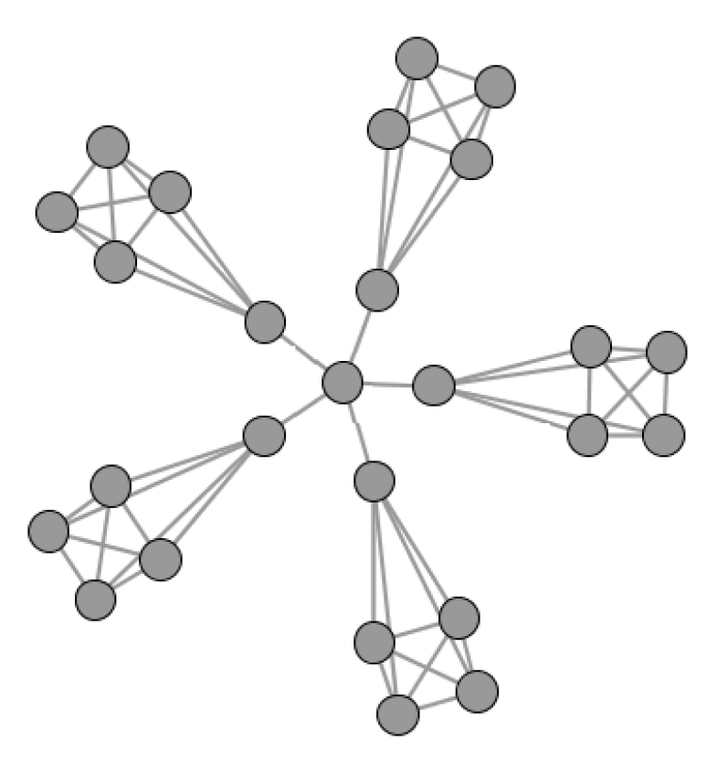
As in preliminary work [
15], consider the star-of-cliques graph family
with
constructed by connecting one central node
to each of
disjoint
-cliques
via
edges of the form
. In particular, for each clique
, there is a unique vertex
that is adjacent to the central vertex
, and we may refer to the set of
vertices adjacent to
as
. An example graph with
is shown in
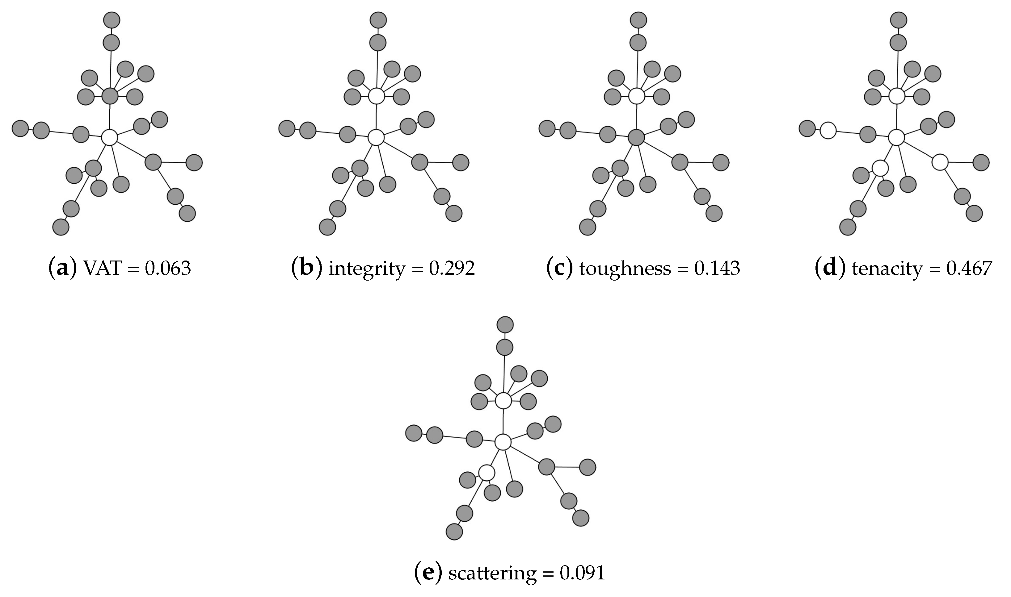
Figure 2. Any reasonable NBR measure for this graph, including all measures considered herein, will output either
or
as the critical attack set
optimizing the NBR measure. As such, the removal of the critical attack set of a node-based resilience measure will result in either exactly
components corresponding identically to the
cliques
or it will result in exactly
components which include the central node and
cliques
. In other words, the computation of a node-based resilience measure results in the immediate partitioning of the star-of-cliques such that every clique corresponds to a distinct cluster, either in its entirety or with only a single node removed.
On the other hand, when considering the conductance of this same star-of-cliques family, it may be observed that, for any setting of , there are several ties for the critical attack set of edges corresponding to conductance: in fact, conductance is minimized by any edge-cutset H that is a subset of and hence cannot adequately cluster this graph. The behavior of modularity is dependent on the parameters and , where there exist settings of those parameters such that modularity will group some of the cliques together into a cluster. For example, if one takes and , then the modularity objective function will result in fewer than 1020 clusters. Therefore, while NBR-measures yield the natural clusters for the star-of-cliques graphs regardless of and , edge-based resilience measures do not.
In addition, we shall now demonstrate that this is also the case for the graph representation of the
hypergraph [
41] with respect to the graph representation mapping hyperedges to cliques [
42]. As defined in [
41], the
star hypergraph has center node
and is formed by some number of hyperedges containing vertex
. When the number of vertices involved in every hyperedge of the star hypergraph is the same number
r, then we obtain the
hypergraph. For consistency of notation here, we may refer to the graph representation of the
hypergraph with
hyperedges and
simply as the graph
. Note that like
,
also involves a central node
connected to
cliques
. However, unlike the star-of-cliques graphs where
is connected to each clique
via a single connection
, in the
graphs the central node
is connected to
all other nodes. Thus, any vertex separator
S for
must include
and is not improved by additional nodes. Therefore, it is straightforward to see that all node-based resilience measures will output only
as the critical attack set for
. We may also observe that the conductance of
suffers a similar problem as the conductance of
, as there are several ties for the critical attack set of edges corresponding to conductance: Letting
denote all the edges connecting
to clique
, for any
, conductance is minimized by edge-cutset
. Hence, conductance cannot adequately cluster
. Finally, regarding the behavior of modularity on
, we again note the dependence on
and
, as well as the specific case
,
providing a counter-example to the efficacy of modularity in detecting all of the clusters, which are naturally the cliques representing the hyperedges.
Therefore, we have exhibited classes of graphs for which NBR-measures output all of the natural clusters although some well-known clustering algorithms based on conductance or modularity may fail to do so. As no clustering algorithm is expected to work perfectly in all scenarios, this is neither a criticism of established clustering methods nor a zealous celebration of the NBR-clustering framework presented herein. Nor have we attempted to exhaustively examine graph families for which NBR–Clust has special positive clustering properties. Rather, we simply solidify our theoretical motivation for the NBR–Clustering framework.
Upon reflection of the star generalizations star-of-cliques and KStar presented above, one sees that the natural belonging of the central node in an attempted clustering is unclear. For example, as in the hypergraph , the central node could naturally represent the overlap of all the clique-clusters, or, as in the star-of-cliques, might be overlap, noise, a cluster of its own, or attached to any existing clique-cluster. Although much of classical clustering research has been dedicated to situations in which a complete partitioning of the vertex set is desired, a body of recent work has been dedicated to examining the reality of incomplete partitionings due to noise or overlap. Based on our theoretical observations consistent with the examples presented herein, we hypothesize the following:
Noise and overlap nodes will tend to be a subset of the critical attack set of meaningful NBR measures.
There exist meaningful NBR measures such that a single computation of the NBR measure and removal of the corresponding critical attack set results in the natural collection component clusters.
In the remainder of this work, we present the specifications of our NBR–Clust framework across disparate scenarios and extensive empirical results supporting both of the above hypotheses. We refer to the second hypothesis as “one shot” clustering, as opposed to the repeated hierarchical applications often required of edge-based methods such as conductance. As a precursor to some of the results that follow, we note that three NBR measures have been found particularly effective in the clustering context: integrity, tenacity, and VAT. Amongst these, integrity and tenacity shall turn out particularly useful for one-shot clustering, with the number of clusters output by tenacity often presenting an upper bound on the ground truth number of clusters. Now, we present our actual framework.
4.1. NBR Clustering Framework
Given a resilience measure R (it is assumed that R expresses a minimization objective taken over possible attack sets of nodes S) and the resilience measure of a specific graph G denoted by , the general NBR measure R-clustering framework, NBR–Clust, is as follows:
- (1)
If not G, transform point data into a graph G.
- (2)
Approximate with an acceptable accuracy, and return candidate attack set S whose removal results in a number of candidate groupings (components).
- (3)
Adjust the number of candidate groupings. If there are too many groups, combine them until the desired number of components is obtained. If there are too few groups, perform hierarchical clustering by proceeding recursively on the component with the lowest resilience value . Continue hierarchical clustering until the desired number of groups is obtained.
- (4)
For a complete (i.e., traditional partition-style) clustering outcome, perform a node-assignment strategy that assigns each node v of S to the component C (from step (3)) in its original semi-partition with which v shares the most edges. Break ties arbitrarily.
- (5)
To cluster in the presence of noise (which implies removal of some nodes identified as noise), remove S. It is possible that some components consist entirely of noise (often significantly smaller components). In such cases, identify and remove those noise components.
- (6)
For clustering of networks with overlap, detect and assign overlap nodes appropriately.
The implementation of this clustering framework is available on the project website [
43].
The NBR–Clust framework has great versatility in that it can be used on many different types of graphs, depending on the resilience measure
R employed in step (2). Classical resilience measures such as those employed in this work are in most cases only meaningful on connected graphs. However, it is shown in [
10] that the measures can be extended to account for disconnected and directed graphs. If a resilience measure can be applied to a particular graph, such as a directed, multi or binary graph, then the NBR–Clustering framework can also be applied. The following sections describe the implementation of parts of the NBR clustering framework.
4.1.1. Transforming Point Data into Graphs
In applying the NBR–Clust framework to point datasets, we first convert the data into a k-nearest neighbor (kNN) graph
G. In a kNN graph
, vertices
u and
v have an edge between them if
v is amongst the
k closest vertices to
u with respect to the distance metric considered. While any distance metric may be used to determine nearness of neighbors, we use the
n-dimensional Euclidean distance, where
n is the number of features considered. Min-conn
k implies choosing the minimal
k such that
. The choice of kNN graphs is motivated by [
6,
44] and empirical evidence from [
15,
19]. Given that NBR measures are meaningful only on connected graphs (the measure VAT has been extended in [
10], such that the VAT of a disconnected graph can be considered to be the minimum VAT of any of its components), the smallest
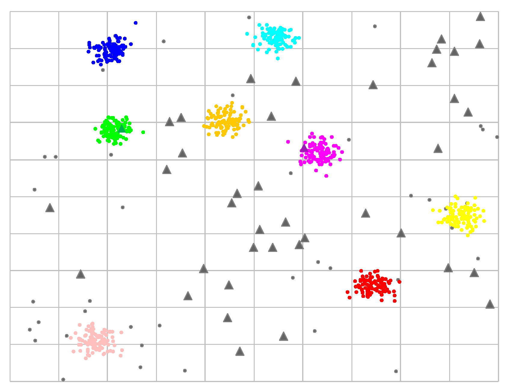
k for which the graph remains connected is chosen. An example of a synthetic point set utilized in this work and its corresponding minimum connectivity kNN graph are shown in
Figure 3 and
Figure 4, respectively.
4.1.2. Joining Clusters
It is possible that fewer clusters are desired than the number obtained from NBR–Clust. Hence, clusters are joined based on their shared edges. For each pair of components
that result from the initial clustering, a normalized cut is computed and defined as follows:
Equation (
9) gives a larger result for smaller components with relatively more edges between them. The two components with the largest result are joined, breaking ties arbitrarily. This creates one fewer component. This process is repeated until the desired number of components is obtained.
4.1.3. Detecting Noise Nodes in Data
When clustering in the presence of noise, the critical attack set
S can be regarded as consisting entirely of noise nodes, as mentioned in step (5) of the NBR–Clust framework. We must also address the possibility of obtaining some clusters that consist of all noise nodes, which we term “all-noise” clusters in addition to
S. These all-noise clusters are usually small compared to the other clusters. They are identified by using separability, a graph-based internal validation measure [
45]. The separability of a set of nodes
P is defined as the ratio of the number of edges in
P to the number of edges on the boundary of
P:
We have found empirically that all-noise clusters have below average separability values. Therefore, we use below-average separability as a threshold value to indicate all-noise clusters.
4.1.4. Identifying and Assigning Overlap Nodes
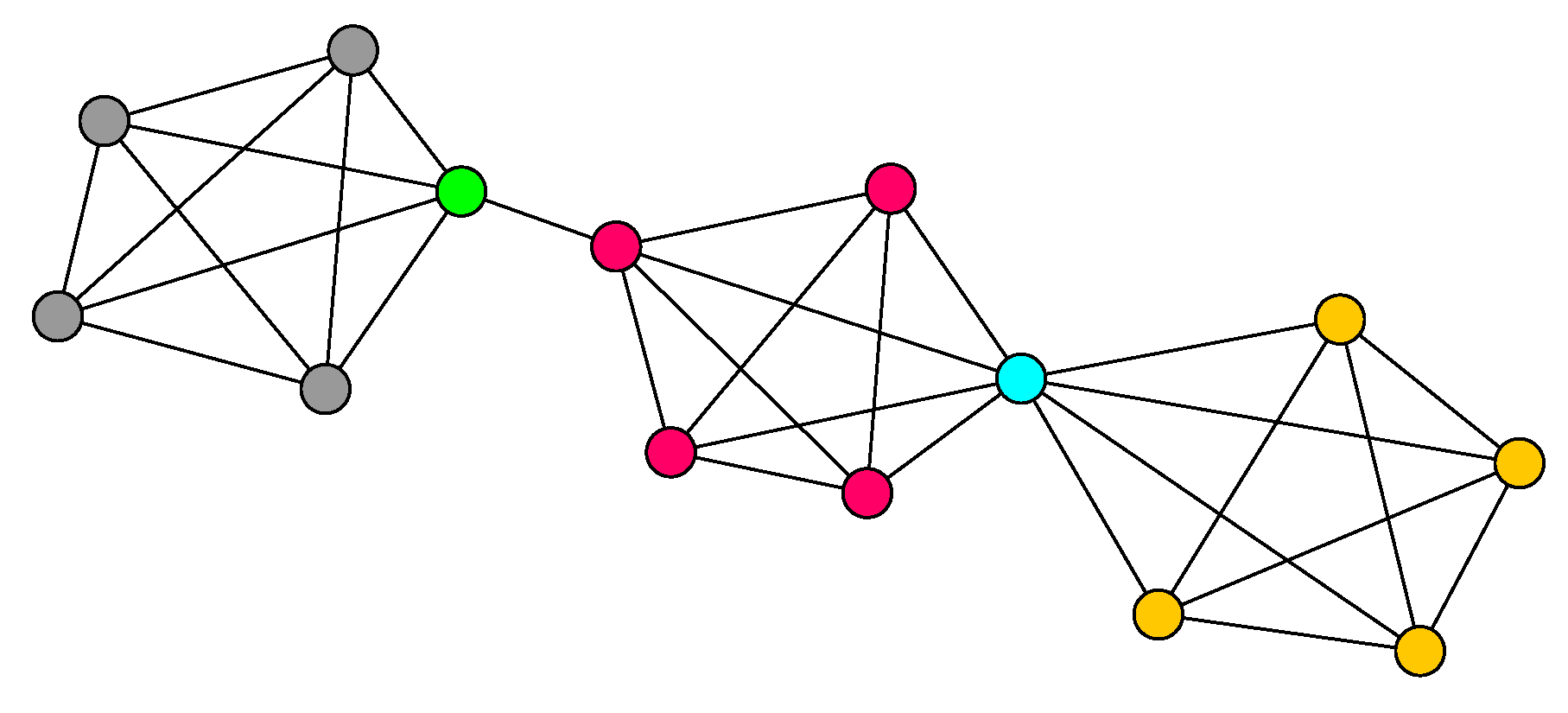
The underlying hypothesis is that overlap nodes (nodes that belong to more than one cluster) are a subset of the critical attack set nodes generated by NBR–Clust. Overlap nodes and attack set nodes share a similar characteristic: both lie on inter-cluster boundaries. In addition, an overlap node maintains a “tight connection” with all its communities [
46]. An overlap node should have equally strong numbers of adjacencies to several communities, while a non-overlap node would display a significantly higher number of adjacencies to one particular community in contrast to others. An example is shown in
Figure 5. Both green and cyan nodes have high betweenness centrality and are likely to be part of a resilience measure critical attack set. The cyan node is determined to be an overlap node because it is tightly connected to both the magenta and yellow communities, and those communities share no other connections. The green node is also connected to two communities but much more tightly to the gray community (four adjacencies) than to the magenta community (only one adjacency). The green node is therefore not an overlap node.
To quantify the strength of a node’s connection to multiple communities, different strategies could be applied. For example, in [
46], overlap nodes are detected using a two-part criterion based not only on adjacencies, but also on a node’s distance from the hubs of the corresponding communities. In [
47], overlap is based on the “distance” from a node to a community, and it is determined with a heuristic that counts the number of triangles between a node and a community.
In this work, the Edge Dispersion Variation (EDV) measure is utilized to quantify how tightly a node
is connected to a given set
Q of communities. The EDV for
, given a set of communities
, is defined as a normalized standard deviation of the percentages of
’s edges that link to
Q’s communities:
where
is the mean of
computed over
Q and
(
) is the percentage of node
’s edges adjacent to
Q that are also adjacent to cluster
i:
The measure of the strength of the connection correlates inversely with the EDV value. Nodes (like the green node in
Figure 5) that are not overlaps will have a higher EDV value.
4.2. Computation of NBR Measures
The existing NP-hardness results for the resilience measures considered in this work include [
48] for integrity (Ref. [
49] for toughness, Ref. [
50] for tenacity, Ref. [
51] for scattering number and [
52] for conductance). The approximation-hardness of unsmoothened vertex attack tolerance (UVAT)
under four separate, plausible computational complexity assumptions was established in [
10,
53]. VAT, integrity, toughness, tenacity and smoothed inverse scattering number are all minimization problems, whose objective functions involve similar calculations of component orders and numbers. Based on the approximation hardness of UVAT, the conjectured hardness of VAT and the previous NP-hardness results for the resilience measures, a greedy betweenness centrality (BC) based algorithm that is similar to the implementation of VAT-Clust presented in [
6], was used to calculate the resilience measures. This greedy BC based heuristic algorithm is detailed in [
10] and referred to as Greedy–BC.
The Greedy–BC algorithm takes graph and set-resilience measure function R as input. Let n denote the total number of nodes in G. The Greedy–BC algorithm is as follows:
Initialize , , , , and .
For to n do:
, and ,
If , then assign
, and
Output as the critical attack set achieving minimum resilience, and as the minimum value achieved for the resilience measure R.
The overall time complexity of the Greedy–BC algorithm depends on the algorithm used to determine the node with the highest BC in each iteration. In general, if that algorithm takes time
, then the overall time complexity of Greedy–BC may be expressed as
. If restricted to exact, deterministic, sequential computational models, the fastest known algorithm to determine the node with the highest BC is Brandes’s Fast Betweenness Centrality algorithm [
54], which takes
time, yielding an overall Greedy–BC time complexity of
. As in [
10], in the context of the work, we implemented Greedy–BC using Brandes’s algorithm [
54] and applied it to all graphs of size up to two thousand vertices. (for graphs with over two thousand vertices, we use a distributed algorithm [
55]).
In [
10], it is experimentally shown that Greedy–BC implemented using Brandes’ betweenness centrality algorithm exhibits excellent empirical approximation bounds for VAT, integrity and tenacity on a representative sample of 24-node graphs, despite the general approximation hardness results for UVAT. In [
6], hill climbing was applied to improve the approximation of the resilience measures; however, it is shown in [
10] that the accuracies of Greedy–BC were not significantly improved by either 1D or 2D hill climbing, even for larger scale-free graphs up to thousands of nodes. The non-parametrized, practical NBR–Clust implementation employed in this work uses Greedy–BC without hill climbing and with unweighted betweenness centrality to
simultaneously approximate VAT, integrity, tenacity, toughness, and scattering in
time.
While Greedy–BC as implemented above yields high clustering accuracy for all graphs studied as well as an improvement in speed over hill-climbing based methods, it is still too slow for applications to very large graphs of tens or hundreds of thousands of nodes. Therefore, we have considered alternative approaches to tackle very large graphs, including parallelized approximations to betweenness centrality [
55] and the use of adaptive approximations [
56].
5. Experimental Results
In this section, we empirically evaluate NBR–Clust on varied datasets and networks to demonstrate the robustness of the algorithm. We quantify performance using the percentage accuracy metric, as well as whether, for a given dataset, the method accurately determines the optimal number of clusters (according to the ground truth). Percentage accuracy is defined as the percentage of nodes correctly clustered for a given dataset.
First, the efficacy of NBR clustering is established by clustering four real native network datasets [
2,
57,
58,
59] and comparing the accuracies obtained by NBR–Clust to two well-known algorithms: Girvan–Newman [
2] and Louvain modularity [
60]. The results of NBR–Clust are also demonstrated on multiple types of synthetically generated graphs with diverse properties including regular and irregular degree graphs such as LFR benchmark networks [
61]. Larger networks of 10,000 and 100,000 nodes are also clustered.
We are very much interested in applications of NBR Clustering for datasets not natively in graph format. To examine that issue, we conduct a comparative analysis of NBR–Clust on sample datasets obtained from the UCI Machine Learning Repository [
62] along with three other algorithms: k-means [
20], Girvan–Newman [
2] and spectral clustering [
3]. We evaluate the performance of NBR–Clust on synthetic datasets generated as multi-dimensional Gaussian mixtures [
63]. Finally, the robustness and effectiveness of NBR clustering methodology in identifying and dealing with noise and overlaps is evaluated and illustrated.
Although this paper’s NBR–Clustering framework is implemented hierarchically, it is noted that in many cases high accuracy is achieved in one shot (without requiring multiple recursive iterations). This suggests there is potential for using some measures to determine a natural number of clusters in a graph when the number of clusters is not known a priori. When clustering has been completed in one step, the percentage accuracy is displayed in bold.
5.1. Real Data in Native Network Form
NBR–Clust using VAT, integrity, toughness, tenacity and scattering number was applied on four sets of data in native network form. The first network represents a set of books about US politics, compiled by Valdis Krebs [
57]. The graph’s nodes represent 105 books sold by Amazon (Seattle, WA 98121, USA), categorized by Mark Newman as liberal, neutral, or conservative. The edges represent frequent co-purchasing of books by the same buyers, as indicated by the
customers who bought this item also bought these other books feature on Amazon. For comparison, Girvan–Newman results for this graph were obtained from [
64], and Louvain modularity [
60] was calculated using Gephi software (version 0.9.2, The Gephi Consortium, from gephi.org, accessed on 30 July 2018). As shown in
Table 1, VAT, integrity, toughness and tenacity all achieved accuracies of 80% or higher on this dataset. Both Girvan–Newman and Louvain modularity attained a clustering accuracy of 84%.
The three additional datasets included Zachary’s karate club [
59], college football [
2] and the Chesapeake Bay food web [
58]. The accuracy results for these datasets are shown in
Table 1. With the karate club, integrity achieves a high accuracy, while VAT and toughness are less successful. Like integrity, Girvan–Newman and Louvain both cluster the karate club at 97%. VAT and integrity achieve high accuracy with the football dataset, correctly classifying at least 89% of the teams according to conference. Girvan–Newman clusters this dataset at 90% accuracy, and Louvain clusters it at 91%. VAT and integrity are the most successful of all methods with the noisy and difficult food web dataset, where both correctly cluster 73% of the nodes. Girvan–Newman clusters the food web at 70%, and Louvain clusters it at 67% accuracy. Note also that, except in two cases with college football, all graphs are clustered by NBR–Clust in one iteration.
5.2. Synthetic Data in Native Network Form
5.2.1. Girvan–Newman Graphs
The Girvan–Newman graphs were generated as described in [
2]. These graphs have 1024 nodes, with either 64, 32, 16 or 8 equal-sized clusters. The graphs have a regular degree structure, with each node’s degree equal to half the cluster size. The strength of the community structure depends on the mixing coefficient,
. Ten different graphs were randomly generated for different mixing coefficients from
to
. However, for this type of graph, higher mixing coefficients are not effective as the resulting graphs are very well connected. Hence, many of the resilience measures do not return a useful attack set.
Nevertheless, these graphs are interesting as they have a very large number of clusters with a small set of members per cluster. For example, each cluster of the 64-cluster graphs contains only 16 members. The large number of clusters implies that either a large critical attack set or a large number of iterations is required. The results for the Girvan–Newman graphs are shown in
Table 2, where # represents the number of clusters in the graph, and
is the mixing factor. Each data point represents an average over 10 randomly generated graphs. As can be observed, NBR–Clust using any measure other than scattering number performs very well on these types of graphs. Even with the most difficult graphs, with the mixing coefficient
, the lowest performance (scattering) is 85% accuracy while all other NBR measures attain at least 92%. Note that tenacity was able to cluster every graph in only one iteration. This is due to the large size of the generated attack sets.
5.2.2. Scale-Free LFR Benchmark Networks of 1024 Nodes
An important generalized class of synthetic networks is the LFR networks [
61]. Note that the networks that may be generated by the LFR model include regular degree Girvan–Newman networks as well as scale-free networks of various parametric settings. A series of LFR benchmark networks was generated as described in [
61]. Each of these graphs has 1024 nodes. In contrast to the regular degree structure of the Girvan–Newman graphs, these are scale-free networks, generated using power law distributions for degree, where the degree sequence exponent =
, and the community size distribution exponent =
. These are similar to real complex networks, which “are known to be characterized by heterogeneous distributions of degree and community sizes” [
65]. Fifty different networks were generated, each containing between 4 and 14 clusters, with the cluster size ranging from 50 to 200 nodes. The degree distributions were highly irregular, with a typical degree distribution ranging from 7 to 64. The average degree was 16. The mixing parameter varied from 0.05 to 0.25, where a higher mixing parameter implies less tightly bound communities, and therefore a more difficult graph to cluster.
The results for the scale-free LFR networks are shown in
Table 3. The average percentage accuracy is presented over 10 separate randomly generated graphs. For graphs with the best-defined community structures (a mixing factor of
), all measures except scattering number correctly classify more than 95% of the nodes. Even where
, toughness and tenacity correctly classify over 85% of the nodes. For this class of graphs, all of the NBR measures, except for scattering, clustered the graphs in one step.
5.2.3. Large LFR Networks
To demonstrate the feasibility of NBR–Clust on larger graphs, two series of LFR networks were generated (10,000 nodes and 100,000 nodes). These networks contain 30 to 40 clusters of varying cluster sizes, ranging from 100 to 500 nodes for the 10,000-node graphs, and 1000 to 5000 nodes for the 100,000-node graphs. The degree distributions are highly irregular, with a typical degree distribution ranging from 20 to 60. Different values of were used ranging from 0.01 to 0.10 for the 10,000-node graphs, and from 0.001 to 0.010 for the 100,000-node graphs. To determine if the number of edges affects the clustering accuracy, two variations of the 100,000-node graphs were tried. One set of graphs had approximately 275,000 edges, and one set had approximately 825,000 edges.
To cluster these larger graphs, Greedy–BC was executed in a distributed fashion using a graphics processing unit (GPU) betweenness centrality approximation algorithm called Hybrid–BC [
55], as described in [
66]. Results are shown in
Table 4. In two cases, the approximation provided by the GPU algorithm was not sufficient to successfully complete clustering with VAT.
With LFR networks, higher mixing factors imply increased difficulty of clustering. Despite the fact that exact betweenness centrality values were not used, clustering accuracies are still quite high. As is shown in
Table 4, 10,000-node graphs with
less than 0.10 were clustered with at least 96% accuracy. To give some idea of execution time, graphs 1 to 5 were clustered in less than five minutes. The last and most difficult graph was clustered in approximately 35 minutes, with 92% accuracy.
Results for the 100,000-node graphs are also shown in
Table 4. Clustering accuracy is high for both the high and low density graphs. Only two of the graphs were clustered with less than 97% accuracy. Clustering times varied a great deal, depending on
and degree. Graphs 1–4 were clustered in less than 30 min, graph 5 took about 2.5 h, and graph 6 took approximately 9.5 h.
5.2.4. Attributed Networks with Communities
A model for generating attributed networks with communities is presented in [
67]. This model is described as “similar to the BTER model” (described in
Section 5.2.5), except that it uses the similarity of the vertex attributes to determine the inter-cluster edges, while BTER uses a scale-free distribution. The results in [
67] suggest that the community structure of these graphs is most affected by the total number of edges in the graph. Fifty graphs were generated with 1000 nodes and 10 clusters (of varying sizes), varying the total number of edges to achieve a specified average degree. The high degree graphs have a strong community structure and should cluster with high accuracies. The low degree graphs should be more difficult to cluster.
Table 5 illustrates the results as an average over 10 multiple graphs generated with the same parameters and average degree. Integrity does especially well on this type of graph, averaging 86% accuracy on the most difficult graphs and 100% accuracy on the easiest. Tenacity clustered every graph in one step, while integrity clustered 48 out of 50 graphs in one step. Additionally, VAT clustered these graphs in an average of two steps or less.
5.2.5. BTER Benchmark
A BTER network [
68] of 1899 nodes was generated using the FEASTPACK Matlab distribution [
69] (version 1.2, Sandia National Laboratories, Albuquerque, NM, USA). In this network model, Erdos–Rényi [
70] communities are created with sizes following a scale-free distribution and then connected with edges chosen according to the Chung and Lu model [
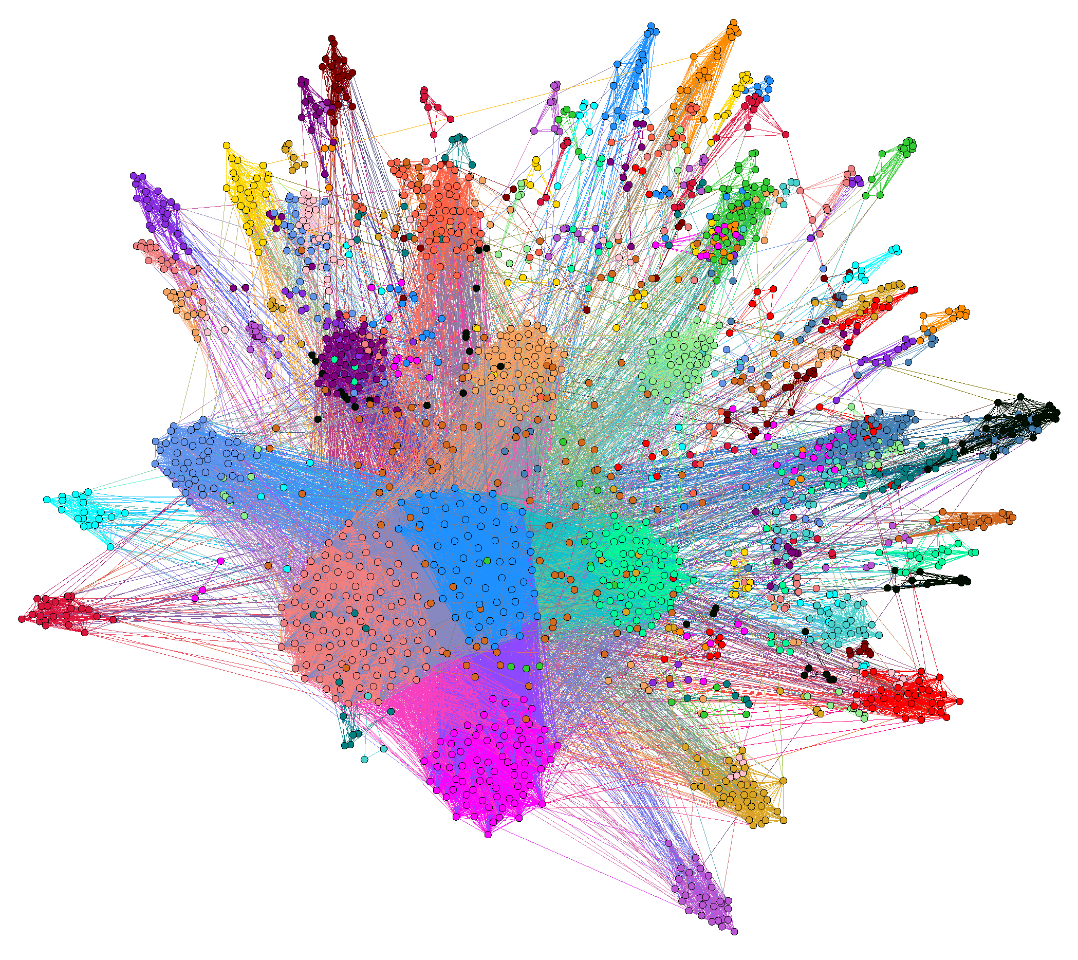
71]. This graph is different from the other tested models because, in addition to having a scale-free degree distribution, the community sizes follow a scale-free distribution. It has 198 clusters. Of these, 47 clusters contain only three nodes, 31 clusters contain four nodes, and the largest cluster contains 101 nodes. The graph is not connected. A visualization of this network is shown in
Figure 6. VAT, integrity and tenacity performed very well on this network with a minimum of 84% accuracy, and all but 5 out of 198 communities were successfully detected. VAT clustered this network at 86% accuracy, and all but 3 of 198 communities were successfully detected.
5.3. Real Data in Point Set Form
The results presented here were obtained by converting point set data into kNN graphs and clustering using NBR–Clust. Four real datasets from the UCI Machine Learning repository [
62] are evaluated: iris, breast-WI,
E.Coli and wine. Percent accuracy for these datasets is shown in
Table 6. VAT, integrity and tenacity generally perform well on these datasets. The matching 90% accuracy of VAT and integrity on the well-known iris dataset is particularly notable, as two of the three iris clusters are not linearly separable. For comparison to existing clustering methods (both point clustering and graph clustering), k-means clusters iris at 89%. The corresponding kNN graph is clustered by spectral clustering at 90% and by Girvan–Newman at 97%. Notably, integrity achieves a high accuracy on iris
in one shot. Integrity and tenacity both clustered all four datasets in one shot.
k-means, spectral clustering, and Girvan–Newman clustered the breast-WI dataset at 85%, 82%, and 77% accuracy, respectively; while the NBR–Clust accuracies ranged from 81% to 85%. For E. coli, the highest accuracy is integrity at 60%, and most measures cluster closer to 55% accuracy. k-means clusters the E. coli dataset at 58% accuracy, spectral clustering at 50% and Girvan–Newman at 61% accuracy. On the wine dataset, NBR–Clust beat k-means and spectral, which clustered at 61% and 70% accuracy, and it tied with Girvan–Newman at 71% accuracy.
5.4. Synthetic Data in Point Set Form
In this section, the performance of NBR–Clust on a set of synthetic datasets generated by Arbelaitz et al. [
63] is evaluated. These datasets were generated as multi-dimensional Gaussian mixtures with either 10% uniformly random noise or no noise. The dimension
D (the number of features of the point set) and the number of clusters
K both vary as 2, 4, or 8. There are nine combinations of
D and
K, shown as one combination per row in
Table 7. Arbelaitz et al. use the term density to describe whether or not the clusters of a dataset are equal in size. In the equal density datasets, each cluster contains 100 members. In the unequal density datasets, one cluster has 400 members, and the remaining clusters have 100 members. For example, a D4K8 equal density dataset has 800 members with no noise, and the corresponding dataset with 10% noise has 880 members. The unequal density D4K8 dataset will have 1100 members with no noise and 1210 members with noise. The Arbelaitz data contains 10 different generated sets of all 9 combinations of D and K, equal and unequal density, noisy and without noise, for a total of 360 datasets.
5.4.1. Synthetic Point Set NBR–Clust Results
The results for clustering the synthetic point set datasets are shown in
Table 7 as an average percent accuracy over the 10 instances per dataset. Toughness and scattering generally performed poorly, hence only the results for VAT, integrity, and tenacity are presented.
VAT attained a high accuracy on all four types of synthetic point set graphs. VAT clustered almost all of the noiseless graphs perfectly, achieving a 99% or 100% average accuracy on each series of 10 graphs. VAT did only slightly worse on the noisy graphs, clustering both equal and unequal density graphs at 95% or above. In general, VAT did not cluster in one step. Clustering took between 1 and 7 steps, and the number of steps did not vary greatly between the four data set variations.
Like VAT, integrity clustered the noiseless datasets almost perfectly, achieving an accuracy of 99% or higher. On the noisy unequal density datasets, integrity did relatively well, clustering between 69% and 95% accuracy. Integrity was less successful with the noisy datasets, although it exhibited a relatively consistent pattern of increasing accuracy as the number of clusters increased, independent of the number of dimensions. Integrity clustered every noisy dataset, and most of the noiseless datasets, in only one iteration.
Tenacity also clustered the non-noisy datasets with high accuracy. Tenacity did not perform as well on the noisy datasets. In contrast to integrity, tenacity performed better on datasets with a smaller number of clusters. Tenacity clustered every dataset in only one step, without requiring further recursive iterations.
5.5. Noise Removal
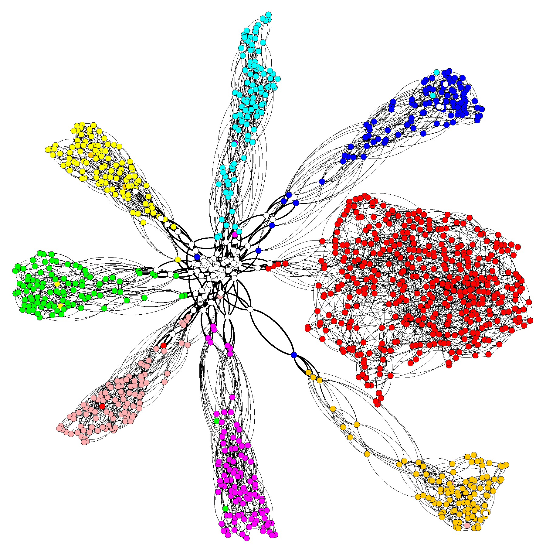
This section specifically evaluates the performance of NBR clustering in removing noise from noisy synthetic datasets, in contrast to the previous section, which presented percentage accuracy results on NBR–Clust’s effectiveness in clustering noisy datasets. The Arbelaitz point set data is utilized, which contains 10% noise that is randomly generated following a “uniform distribution over the sampling window” [
63]. A visualization of an unequal density dataset with noise is illustrated in
Figure 7. The cases of primary interest are those where NBR–Clust successfully removes noise without compromising clustering accuracy, and it is preferred if this is accomplished in one iteration.
The measures precision and recall are used to quantify NBR–Clust performance when identifying noise nodes. Let denote the number of noise nodes in the dataset; , the number of nodes in the critical attack set; and , the number of noise nodes contained in that attack set. Precision is defined as P = , and recall is defined as RC = . Precision indicates how successful the algorithm was in identifying the noise nodes as the attack set nodes, while recall is the percentage of the overall noise nodes that were contained in the attack set.
Table 8 shows the precision and recall of NBR–Clust using VAT, integrity and tenacity when removing noise from noisy datasets. Integrity gives the most balanced mix of precision and recall. VAT generally has a high precision—the nodes it finds are quite likely to be noise nodes, but due to the smaller attack set sizes, it does not find a large percentage of noise nodes. Tenacity has the opposite problem, often finding over 90% of noise nodes, but also with the high probability that many of them are not noise, implying low precision but high recall.
7. Discussion
The theoretical motivation for a generalized NBR clustering framework is based on the relationship between resilience and clustering. This relationship is explicit in the sparsest cuts clustering framework, and has been extended in a novel manner to NBR measures, which presents unique challenges as well as advantages for noise removal and overlapping community detection. This paper’s theoretical motivation is strengthened by defining an infinite family of graphs, as illustrated in
Figure 2, such that using any node-based resilience measure for clustering immediately (in one iteration) yields the correct partitions. Furthermore, a generalized node-based resilience clustering framework (NBR–Clust) is presented that is naturally applicable for variations of the traditional clustering problem in which a complete partitioning is not appropriate, such as clustering in the presence of noise as well as in the presence of overlapping clusters.
The primary goal of this work has been to demonstrate the effectiveness of NBR–Clustering methodology via extensive experimental results across variations of the clustering problem and a diverse set of datasets, including real and synthetic, as well as native graph data and point set data. There are computational hardness results pertaining to all resilience measures considered in this research’s NBR–Clustering framework. The heuristic,
time Greedy–BC method is utilized to
simultaneously compute all relevant measures given the acceptable empirical approximation factors attained for that approach in [
10] as well as the super-linear improvement in the time complexity of Greedy–BC over Greedy–BC with hill-climbing. Additionally, use of a parallelized algorithm as described in [
55] allowed the clustering of larger graphs of up to 100,000 nodes in reasonable times. In the context of this work, the main concern is the quality of the clusterings obtained via NBR–Clustering as well as examination of NBR measures and data scenarios for which NBR–Clustering performs (i) accurate one-iteration clustering without the number of clusters known a priori; (ii) noise removal with high precision and recall and (iii) high-quality detection of overlapping communities.
NBR–Clust exhibited competitive results compared to the popular Girvan–Newman and Louvain community detection methods on a series of well-known real networks, outperforming those methods on the food web dataset and tying them on the karate club network. Regarding performance on synthetic graph data, this paper has demonstrated that NBR–Clust gives robust results for both regular and scale-free degree distributions, for varying cluster size distributions, across a reasonable range of mixing factors, and even on complex networks with attributes. NBR–Clustering results on real and synthetic datasets generated from point-set data transformed into kNN graphs have been similarly promising, both in noiseless and noisy (10% uniformly random noise) settings. On a series of kNN graphs generated from Gaussian-mixture point-set data, VAT, integrity and tenacity clustered noiseless datasets almost perfectly, with VAT also clustering all noisy point-set data almost perfectly. VAT also resulted in accurate clustering for the BTER complex network dataset. Although the BTER network’s scale-free distribution of both cluster size and degree is known to cause difficulty for many clustering algorithms, NBR–Clustering, using VAT, was able to detect all but 3 of 198 clusters.
While VAT has been particularly notable in accurate clustering across various datasets, integrity and tenacity have shown promise in one step clustering across a variety of network and point set data when the number of clusters is unknown a priori. Both integrity and tenacity clustered all attributed network datasets in a single iteration, with integrity clustering at an average of 86% accuracy. For the LFR benchmarks, attributed networks with communities and synthetic point set graphs, integrity clustered 42 out of 46 sets (of 10 graphs) in only one step. Tenacity clustered every regular Girvan–Newman graph in one step with an average accuracy greater than 92%. Tenacity also clustered every kNN graph generated from noiseless and noisy synthetic point set data in one step, and integrity clustered the majority of such data sets in one step with relatively higher accuracies. Upon closer examination of the poor performance of tenacity on noisy synthetic datasets, it was observed that many more nodes were removed by tenacity (including many non-noise nodes), resulting in a higher number of clusters than necessary. Thus, even in cases where tenacity does not achieve an accurate clustering in one step, the number of clusters formed by tenacity serves as an upper bound on the correct number of clusters desired. Finally, in the context of clustering in a single iteration, this research shows that, for all measures except scattering, NBR–Clust clustered almost every scale-free LFR benchmark network in a single iteration.
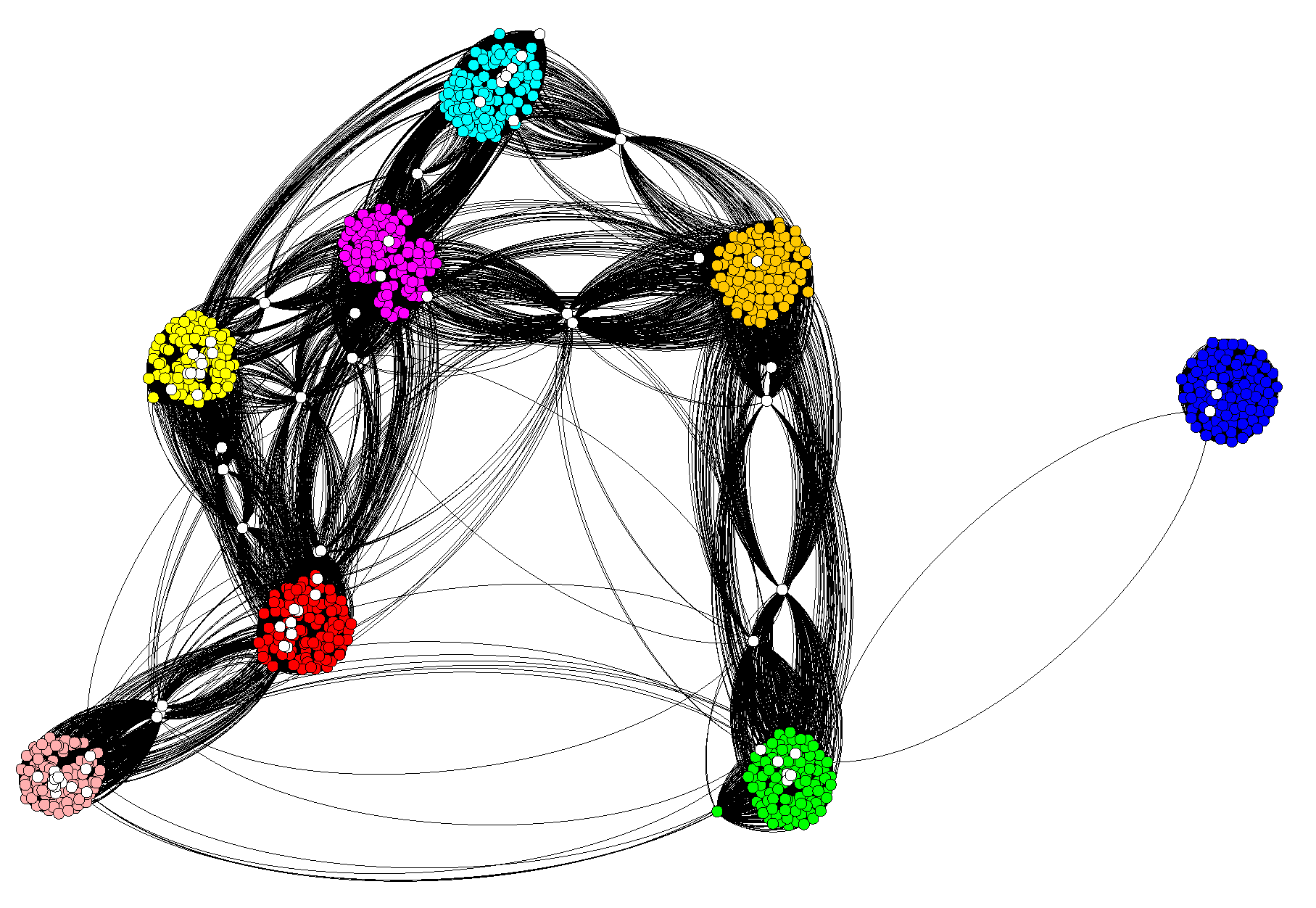
Another important contribution of this work is the application to noise removal. The efficacy of NBR–Clust has been examined with respect to noise removal which occurs as an automatic by-product of node-based resilience measure computation, particularly computation of the critical attack set, which is taken as a candidate set of noise nodes. As stated previously, the noisy datasets of this work are minimum connectivity kNN graphs with Gaussian mixture ground truth clusters and an additional 10% uniformly random noise. VAT showed high precision in detecting noise nodes, with the percentage of noise nodes in the critical attack sets ranging from 63% to 94%. VAT’s small attack set size implied that the total number of noise nodes found was small. In contrast, tenacity generally detected over 90% of the noise nodes, but with low precision. Integrity had the best combination of precision and recall with noise detection, although results varied. Noise removal with one-shot integrity-based partial clustering was particularly notable on two classes of noisy point sets: equal density D4K8 and equal density D8K8. For the D4K8 datasets, integrity identified approximately 50% of the noise nodes, with a precision of 96%, while still retaining one-shot clustering accuracies of 97% and 100%. It is interesting to consider the graph corresponding to the noisy, D8K8 unequal density dataset shown in
Figure 7. The central location of the noise nodes in this scenario yields a natural stochastic generalization of this paper’s illustrative example motivating node-based resilience measures for partial clustering in
Figure 2.
It is not necessary for the noise to form a single centrally located group in order for NBR clustering to cluster effectively. For example, consider the noisy, equal density D2K8 dataset shown in
Figure 3. Attack-set noise nodes are shown as triangles, and the corresponding min-conn kNN graph is shown in
Figure 4. All NBR measures, except scattering, clustered the graph perfectly. The noise removal on that dataset was also at least 49% for all resilience measures considered. It can be observed that the uniformly at random distributed noise still tends to form high-betweenness nodes “between” natural clusters.
Finally, this paper discusses the effectiveness of NBR–Clust with respect to overlapping communities. There are relatively few algorithms that can account for overlap. The hypothesis motivating the application of node-based resilience for this setting was that overlap nodes would be a subset of attack set nodes because they both lie on inter-cluster boundaries. This hypothesis has been strongly supported by this paper’s experiments as the attack sets contained, on average, at least 99% of the overlap nodes across all datasets with overlapping communities.
On regular Girvan–Newman graphs with overlapping communities, NBR–Clust results with VAT and integrity have been promising for lower mixing factors, as both measures have clustered such graphs with at least 0.94 NMI. Amongst the Girvan–Newman graphs with overlap, the most difficult clustering situations had 32 of 256 nodes overlapping 6 out of 13 clusters, and VAT still achieved an NMI of 0.83, while integrity scored 0.81. The results are similarly notable for integrity on scale-free benchmark graphs with overlap. Integrity achieved high NMI scores while clustering every graph in one step. In the case where 100 nodes overlapped six clusters each, integrity scored an NMI of 0.84. In this case, an average of less than 2% of the nodes were misidentified (and incorrectly assigned to clusters).
As far as assignment of overlap nodes is concerned, one of the problems of overlap clustering algorithms in general is that the overlaps make distinct clusters difficult to determine. Approaches such as maximizing modularity must consider many different options and do not have deterministic outcomes. One of the benefits of NBR–Clust is that the initial clusters are both disjoint (because overlaps have been removed as part of the attack set) and reflective of the natural number of clusters of the graph, so that critical node assignment can be a low time complexity, deterministic process. Due to such inherent properties of critical attack sets for node-based resilience measures, this research demonstrates that a straightforward adjacency-based approach yields a successful strategy to subsequently assign the overlapping nodes to multiple clusters after the critical attack set computation.

 ,
, 

