Consideration of GLONASS Inter-Frequency Code Biases in Precise Point Positioning (PPP) International Time Transfer

Abstract

International time transfer based on Global Navigation Satellite System (GLONASS) precise point positioning (PPP) is influenced by inter-frequency code biases (IFCBs) because of the application of frequency division multiple access technique. This work seeks to gain insight into the influence of GLONASS IFCBs on international time transfer based on GLONASS-only PPP. With a re-parameterization process, three IFCB handling schemes are proposed: neglecting IFCBs, estimating IFCB for each GLONASS frequency number, and estimating IFCB for each GLONASS satellite. Observation data collected from 39 globally distributed stations in a 71-day period (DOY 227–297, 2017) was exclusively processed. For the comparison reason, Global Positioning System (GPS)-only PPP solutions were regarded as reference values. The clock differences derived from GPS- and GLONASS-only PPP solutions were then analyzed. The experimental results demonstrated that considering GLONASS IFCBs could reduce standard deviation (STD) of the clock differences for both identical receiver types and mixed receiver types, of which reduction was from 3.3% to 62.6%. Furthermore, compared with neglecting IFCBs, STD of the clock differences with estimating IFCB for each GLONASS satellite in coordinate-fixed mode was reduced by more than 30% from 0.30 to 0.20 ns, and by 10% from 0.40 to 0.35 ns, for 1-day arc solutions and 10-day arc solutions, respectively. Moreover, different precise products from three International GNSS Service (IGS) analysis centers were also evaluated. Even though different IFCB handling schemes were adopted in GLONASS satellite clock estimation, our numerical results showed that international time transfer on the basis of estimating IFCB for each GLONASS satellite better than the other two processing schemes. To achieve high-precision GLONASS-only PPP-based international time transfer, it is highly recommended to estimate IFCB for each GLONASS satellite.

1. Introduction

The GPS, as one of Global Navigation Satellite Systems (GNSSs), was first applied for time transfer by Allan and Weiss [1] in the 1980s. Afterwards, a technique called Common-View (CV) was employed for International Atomic Time (TAI) comparison. This method provided an opportunity for high-precision (several nanoseconds) time transfer with a low-cost receiver [1]. Furthermore, with development of the precise products released by the International GNSS Service (IGS) [2,3], precise point positioning (PPP) approach, using phase and code observations, was applied for time and frequency transfer in the time community [4,5,6]. PPP has been utilized to compute time links for TAI since September 2009 and is currently used by upon 50% of more than 70 laboratories in the word contributing to TAI and Universal Time Coordinated (UTC) computation [7,8]. Compared with GNSS code-only techniques, such as CV and All-in-View (AV) [9], better short-term stability in time transfer can be achieve with PPP. The present typical uncertainty of PPP-based frequency comparison is about 1 × 10⁻¹⁵ at 1-day average and about 1 × 10⁻¹⁶ at 30-day average, where corresponding to type A uncertainty of 0.3 ns for time-links in the Bureau International des Poids et Mesures (BIPM) Circular T. Moreover, the integer-PPP (IPPP) technique implemented by CNES (Centre National d’Etudes Spatiales) was first applied to perform frequency transfer [10]. The results demonstrated that the IPPP technique allowed frequency comparison with 1 × 10⁻¹⁶ accuracy in several days and could be readily operated with existing products.

With multi-GNSS development, multi-GNSS techniques are widely utilized in timing community. The second GNSS, Russia’s GLONASS, has been reinvigorated since October 2011 and is now fully operational with 24 satellites. Furthermore, the number of IGS stations, which can track GLONASS satellites, is increasing [11]. Hence, researchers have begun to investigate the performances of GLONASS positioning [12,13], ionospheric studies [14,15], tropospheric studies [16] and time transfer [17]. Unlike GPS, the GLONASS carrier phase and pseudorange observations suffer from different frequencies and inter-frequency biases due to the signal structure of GLONASS, which is based on the frequency division multipath access technique [18]. Many studies have investigated the feature of inter-frequency phase biases (IFPBs) and indicated that a liner function of the frequency number can be employed to model the IFPBs [19,20]. Moreover, several studies investigated the characteristics of inter-frequency code biases (IFCBs) and demonstrated that IFCBs were dependent on receiver types, antenna types, domes and firmware versions [21,22]. GLONASS pseudorange observations usually set a very small weight to reduce the effect of IFCBs [12]. However, this assignment will significantly reduce the contribution of pseudorange observations on PPP solutions, especially in the initialization phase. Hence, proper modeling of IFCBs is essential and critical for GLONASS-only PPP-based international time transfer.

To fully understand GLONASS IFCBs, Shi et al. [21] estimated the IFCBs using GPS/GLONASS observations about 133 stations. Their study demonstrated that the IFCBs of some receivers showed a linear function of frequency numbers, while other showed a quadratic polynomial function. Chen et al. [23] employed different IFCB handling schemes in GPS/GLONASS satellite clock estimation, giving the conclusion that considering GLONASS IFCBs can achieve better positioning performance of GPS/GLONASS PPP. Furthermore, Zhou et al. [13] investigated the influence of GLONASS IFCBs on convergence time and positioning performance of GLONASS-only and GPS/GLONASS PPP, suggesting that the convergence of PPP will be reduced using GLONASS observations by more than 20% when considering IFCBs.

To date, only a few studies have focused on combined GPS/GLONASS time transfer [17,24]. For example, Defraigne and Baire [25] displayed a simple GPS/GLONASS PPP time transfer. Their study showed that adding GLONASS observations could modify the shape of the curve and improve the short-term stability slightly. Up to now, limited studies focus on international time transfer on the basis of GLONASS-only PPP with considering IFCBs. This contribution seeks to gain insight into the influence of GLONASS IFCBs on international time transfer based on GLONASS-only PPP. PPP strongly depends on the externally final orbit and clock products.

Table 1. Global Navigation Satellite System (GLONASS) inter-frequency code bias (IFCB) handling schemes of three International GNSS Service (IGS) analysis centers (ACs) in GLONASS satellite clock offset estimation.

ACs	Scheme	Source of Handling Scheme
COD	Estimate IFCB for each GLONASS satellite	Prange, Orliac [26]
ESA	Estimate IFCB for each GLONASS satellite	ftp://igs.org/pub/center/analysis/esa.acn. Line 406
GFZ	Estimate IFCB for each GLONASS frequency number	ftp://igs.org/pub/resource/pubs/2011_techreport.pdf. Page 61, line 21

summarizes the IFCB handling schemes adopted by different IGS analysis centers (ACs) in GLONASS satellite clock estimation. In this contribution, three GLONASS IFCB handling schemes, which are neglect IFCBs, estimate IFCB for each GLONASS frequency number, and estimate IFCB for each GLONASS satellite, are employed into our ionospheric-free PPP model. The remaining paper is conducted as follows. It starts with a representation of GLONASS ionospheric-free PPP model considering IFCBs in detail. The data selection and processing strategies are then introduced. Afterwards, in accordance with the uncertainty indicator, the performance of PPP-base time transfer by using different receiver and antennas, different processing modes (with/without fixing coordinates), and different precise products is evaluated. Finally, it ends with summary and conclusions.

2. Theory of GLONASS Ionospheric-Free PPP Models

GLONASS undifferenced pseudorange and carrier-phase observations are described. The processing schemes of GLONASS IFCBs are then introduced.

2.1. GLONASS PPP Observation Model

The GLONASS undifferenced pseudorange P and carrier phase L observations can generally be written as [13]

$$\{\begin{array}{l}{P}_{r,j}^s={\rho }_r^s+c\cdot d{t}_r-c\cdot d{t}^s+M{F}_w(e)\cdot Z_w+I_{r,j}^s+\left(d_{r,j}^s-d_j^s\right)+{\epsilon }_{r,j}^s\left(P\right)\\ L_{r,j}^s={\lambda }_j^s\cdot {\varphi }_{r,j}^s\\ ={\rho }_r^s+c\cdot d{t}_r-c\cdot d{t}^s+M{F}_w(e)\cdot Z_w-I_{r,j}^s+{\lambda }_j^s\cdot \left(N_{r,j}^s+B_{r,j}^s-B_j^s\right)+{\epsilon }_{r,j}^s\left(\varphi \right)\end{array}$$

(1)

where the superscript s refers to the GLONASS satellites ID; the subscripts r and j (j = 1, 2) denote the receiver and frequency band, respectively; L and P are the carrier phase and pseudorange observations, respectively; ${\lambda }_j^s$ is the carrier wavelength on the frequency band f_j; $\rho$ is the geometric distance; c is the speed of light; dt_r and dt^s denote the clock error of the receiver and satellite, respectively; e refer to the elevation angle of the satellite s; MF_w is the wet mapping function; Z_w is the zenith wet delay; $I_{r,j}^s$ is the slant ionospheric delay on the frequency j; $d_j^s$ and $d_{r,j}^s$ refer to the uncalibrated code delay (UCD) at satellite and receiver end, respectively; $B_{r,j}^s$ and $B_j^s$ represent the uncalibrated phase delay (UPD) at receiver and satellite end, respectively; ${\epsilon }_{r,j}^s\left(P\right)$ and ${\epsilon }_{r,j}^s\left(\varphi \right)$ represent the observation noise; N donates the integer phase ambiguity.

In our study, the dual-frequency ionosphere-free observations are employed to weaken the effect of the first-order ionospheric delay and can be written as

$$\{\begin{array}{l}{P}_{IF,r}^s=\frac{f_1^2\cdot P_1^s-f_2^2\cdot P_2^s}{f_1^2-f_2^2}\\ L_{IF,r}^s=\frac{f_1^2\cdot L_1^s-f_2^2\cdot L_2^s}{f_1^2-f_2^2}\end{array}$$

(2)

where P_IF and L_IF refer to the ionosphere-free pseudorange and carrier-phase observations, respectively. P_i and L_i are pseudorange and carrier-phase observations on the ith (i = 1, 2) frequency. Since the precise satellite clock products are derived from the L₁/L₂ ionospheric-free observations. The ionospheric-free UCD in pseudorange observations will be absorbed by the precise satellite clock ($c\cdot d_{I{F}_{12}}^s$), which reads

$$\{\begin{array}{c}\alpha =\frac{f_m^2}{f_m^2-f_n^2}\\ \beta =-\frac{f_n^2}{f_m^2-f_n^2}\\ \begin{array}{l}c\cdot d{t}_{I{F}_{12}}^s=c\cdot d{t}^s+\alpha \cdot d_1^s+\beta \cdot d_2^s\\ =c\cdot d{t}^s+d_{I{F}_{12}}^s\end{array}\end{array}$$

(3)

where $\alpha$ and $\beta$ are frequency-dependent factors (m, n = 1, 2; m $\ne$ n).

Substituting (2) and (3) into (1), the GLONASS observation model can be expressed as

$$\{\begin{array}{l}{P}_{I{F}_{12},r}^s={\rho }_r^s+c\cdot d{t}_r-c\cdot d{t}_{I{F}_{12}}^s+M{F}_w(e)\cdot Z_w+d_{r,I{F}_{12}}^s+{\epsilon }_{r,I{F}_{12}}^s\left(P\right)\\ L_{I{F}_{12},r}^s={\lambda }_{I{F}_{12}}^s\cdot {\varphi }_{r,I{F}_{12}}^s\\ ={\rho }_r^s+c\cdot d{t}_r-c\cdot d{t}_{I{F}_{12}}^s+d_{I{F}_{12}}^s+M{F}_w(e)\cdot Z_w+{\lambda }_{I{F}_{12}}^s\cdot \left(N_{r,I{F}_{12}}^s+B_{r,I{F}_{12}}^s-B_{I{F}_{12}}^s\right)+{\epsilon }_{r,I{F}_{12}}^s\left(\varphi \right)\end{array}$$

(4)

with $d_{r,I{F}_{12}}^s=\alpha \cdot d_{r,1}^s+\beta \cdot d_{r,1}^s$; $B_{r,I{F}_{12}}^s=\alpha \cdot B_{r,1}^s+\beta \cdot B_{r,2}^s$; $B_{I{F}_{12}}^s=\alpha \cdot B_1^s+\beta \cdot B_2^s$.

2.2. Handling Schemes of GLONASS IFCBs

Generally, GLONASS IFCBs vary with each satellite. If improperly modeled, a part of the IFCBs will be absorbed by receiver clocks, and the remaining residual biases will degrade the uncertainty of time transfer. To overcome this problematic issue, three handling schemes of IFCBs are proposed [27].

• Neglecting IFCBs. When neglecting IFCBs, a part of IFCBs is absorbed by the parameters of the receiver clock offset. The remaining IFCBs will be reflected in the pseudorange residual. The parameter vector of (4) can be conducted as

  $$\{\begin{array}{l}c\cdot d{\overline{t}}_r=c\cdot d{t}_r+d_{r,I{F}_{12}}^{s,0}\\ {\overline{N}}_{r,I{F}_{12}}^s={\lambda }_{I{F}_{12}}^s\cdot \left(N_{r,I{F}_{12}}^s+B_{r,I{F}_{12}}^s-B_{I{F}_{12}}^s\right)+d_{I{F}_{12}}^s-\\ X={\left[x,c\cdot d{\overline{t}}_r^{},Z_w,{\overline{N}}_{I{F}_{12}}^{}\right]}^T\end{array}{d}_{r,I{F}_{12}}^{s,0}$$

  (5)

  with X the parameter vector of the model; x denotes the vector of the receiver position increments.
• Separating IFCBs by signal frequencies. We set an IFCB parameter to each GLONASS satellite with the same frequency number. The IFCBs are written as follows

  $$d_{r,j}^R=d_{r,j}^{R,0}+K_{}^i\cdot {\nabla }_{r,j}^{i,R}$$

  (6)

  where $d_{r,j}^{R,0}$ refer to the IFCB for the satellite, which frequency number is 0; $K_{}^i$ is the frequency number (−7~6); ${\nabla }_{r,j}^R$ indicates the part of IFCB that depend on the frequency number. Note that the necessary zero-mean condition for the improvements of all relevant parameters are automatically applied.

  $$\{\begin{array}{l}{\nabla }_{r,I{F}_{12}}^s=\alpha \cdot {\nabla }_{r,1}^s+\beta \cdot {\nabla }_{r,2}^{i,s}\\ {\displaystyle \sum _i^n{\nabla }_{r,I{F}_{12}}^{i,s}}=0\end{array}$$

  (7)

  with n the number of the GLONASS frequency. The parameter vector of (4) is conducted as follows:

  $$\{\begin{array}{l}c\cdot d{\overline{t}}_r=c\cdot d{t}_r+d_{r,I{F}_{12}}^{R,0}\\ {\overline{N}}_{r,I{F}_{12}}^R={\lambda }_{I{F}_{12}}^R\cdot \left(N_{r,I{F}_{12}}^R+B_{r,I{F}_{12}}^R-B_{I{F}_{12}}^R\right)+d_{I{F}_{12}}^R-d_{r,I{F}_{12}}^R-K^i{\nabla }_{r,I{F}_{12}}^{i,R}\\ X={\left[x,c\cdot d{\overline{t}}_r^{},Z_w,{\overline{N}}_{r,I{F}_{12}}^R,K^i{\nabla }_{r,I{F}_{12}}^{i,R}\right]}^T\end{array}$$

  (8)
• Separating the IFCBs by GLONASS satellites. The IFCBs are modelled as follows:

  $$d_{r,j}^R=d_{r,j}^{R,0}+{\mathsf{\Omega }}_{r,j}^{i,R}$$

  (9)
  The necessary zero-mean condition for the improvements of all relevant parameters are automatically applied.

  $$\{\begin{array}{l}{\mathsf{\Omega }}_{r,I{F}_{12}}^s=\alpha \cdot {\mathsf{\Omega }}_{r,1}^s+\beta \cdot {\mathsf{\Omega }}_{r,2}^{i,s}\\ {\displaystyle \sum _k^n{\mathsf{\Omega }}_{r,I{F}_{12}}^{k,s}}=0\end{array}$$

  (10)

  where n again denotes the number of GLONASS satellites; k is satellite number. Twenty-four constraints exist per day due to 24 GLONASS satellites in each day of 2017. The condition suggests that the IFCBs are not considered to be dependent on a specific GLONASS frequency number. The parameter vector of (4) is conducted as

  $$\{\begin{array}{l}c\cdot d{\overline{t}}_r=c\cdot d{t}_r+d_{r,I{F}_{12}}^{R,0}\\ {\overline{N}}_{r,I{F}_{12}}^R={\lambda }_{I{F}_{12}}^R\cdot \left(N_{r,I{F}_{12}}^R+B_{r,I{F}_{12}}^R-B_{I{F}_{12}}^R\right)+d_{I{F}_{12}}^R-d_{r,I{F}_{12}}^R-{\mathsf{\Omega }}_{r,I{F}_{12}}^{i,R}\\ X={\left[x,c\cdot d{\overline{t}}_r^{},Z_w,{\overline{N}}_{r,I{F}_{12}}^R,{\mathsf{\Omega }}_{r,I{F}_{12}}^{i,R}\right]}^T\end{array}$$

  (11)

3. Materials and Methods

To investigate the impact of IFCBs on GLONASS PPP-based international time transfer, observation data from the IGS tracking network and timekeeping laboratory were selected. Furthermore, data processing strategies are described in detail.

3.1. Experimental Datasets

In order to validate the processing schemes of the GLONASS IFCBs on PPP-based time transfer, observations from 36 IGS stations and three stations of the time-keeping laboratory were chosen, which covered a 71-day period of Day of Year (DOY) 227–297 in 2017. The selected stations are equipped with receivers from seven manufacturers (see

Table 2. Summary of Global Navigation Satellite Systems (GNSS) receivers of the selected stations.

Manufacturer	Receiver Type	Number of Stations
JAVAD	TRE_G3TH DELTA	10
LEICA	GR10	1
	GR25	1
	GRX1200 + GNSS	1
	GRX1200GGPRO	1
NOV	OEM6	1
SEPT	POLARX3ETR	1
	POLARX4	7
	POLARX4TR	8
TPS	NETG3	1
TRIMBLE	NETR8	1
	NETR9	6
SUM		39

). The detail information of these stations is listed in

Table 3. The detail information of selected IGS stations.

Site	Long Name	Clock	Receiver	Receiver Firmware	Antenna
AGGO	AGGO00ARG	CESIUM	LEICA GR25	3.11	TRM57971.00
ALBH	ALBH00CAN	H-MASER	TPS NET-G3A	4.02	TRM57971.00
BOR1	BOR100POL	H-MASER	TRIMBLE NETR9	5.2	TRM59800.00
BRUX	BRUX00BEL	CH1-75A MASER	SEPT POLARX4TR	2.9.6	JAVRINGANT_DM
CEBR	CEBR00ESP	H-MASER	SEPT POLARX4TR	2.9.5	SEPCHOKE_MC
DLF1	DLF100NLD	CESIUM	TRIMBLE NETR9	5.15	LEIAR25.R3
DRAO	DRAO00CAN	H-MASER	JAVAD TRE_G3TH DELTA	3.6.3	TRM59800.00
GOP6	GOP600CZE	CESIUM	LEICA GRX1200 + GNSS	9.20/6.405	LEIAR25.R4
HERS	HERS00GBR	H-MASER	SEPT POLARX3ETR	2.1	LEIAR25.R3
KIRU	KIRU00SWE	CESIUM	SEPT POLARX4	2.9.5	SEPCHOKE_MC
KOUR	KOUR00GUF	H-MASER	SEPT POLARX4	2.9.5	SEPCHOKE_MC
MAS1	MAS100ESP	CESIUM	SEPT POLARX4	2.9.5	LEIAR25.R4
MATE	MATE00ITA	H-MASER	LEICA GRX1200GGPRO	8.71/3.823	LEIAT504GG
MEDI	MEDI00ITA	H-MASER	LEICA GR10	4.02/6.522	LEIAR20
MGUE	MGUE00ARG	H-MASER	SEPT POLARX4	2.9.5	LEIAR25.R4
MIZU	MIZU00JPN	CESIUM	JAVAD TRE_G3TH DELTA	3.6.7	JAV_RINGANT_G3T
MKEA	MKEA00USA	H-MASER	JAVAD TRE_G3TH DELTA	3.6.4	JAVRINGANT_DM
NRC1	NRC100CAN	H-MASER	JAVAD TRE_G3TH DELTA	3.6.3	AOAD/M_T
NYA1	NYA100NOR	H-MASER	TRIMBLE NETR8	48.01	ASH701073.1
OHI3	OHI300ATA	H-MASER	LEICA GR25	4.10/6.523	LEIAR25.R4
ONSA	ONSA00SWE	H-MASER	JAVAD TRE_G3TH DELTA	3.5.12	AOAD/M_B
PARK	PARK00AUS	H-MASER	TRIMBLE NETR9	5.15	ASH701945C_M
PIE1	PIE100USA	H-MASER	JAVAD TRE_G3TH DELTA	3.6.4	ASH701945E_M
PRDS	PRDS00CAN	H-MASER	JAVAD TRE_G3TH DELTA	3.6.3	AOAD/M_T
PT11		H-MASER	SEPT POLARX4TR	2.9.6	H-MASER
REDU	REDU00BEL	CESIUM	SEPT POLARX4	2.9.5	SEPCHOKE_MC
ROAP	ROAP00ESP	H-MASER	SEPT POLARX4TR	2.9.0	LEIAR25.R4
SPT0	SPT000SWE	H-MASER	JAVAD TRE_G3TH DELTA	3.5.12	JNSCR_C146-22-1
STK2	STK200JPN	CESIUM	TRIMBLE NETR9	4.61	TRM59800.00
SYDN	SYDN00AUS	CESIUM	SEPT POLARX4TR	2.9.6	ASH701945C_M
TSK2	STK200JPN	H-MASER	TRIMBLE NETR9	4.61	TRM59800.00
USN9	USN900USA	H-MASER	NOV OEM6	OEM060000RN0000	TPSCR.G5
VILL	VILL00ESP	CESIUM	SEPT POLARX4	2.9.5	SEPCHOKE_MC
WTZS	WTZS00DEU	CESIUM	SEPT POLARX4TR	2.9.3	LEIAR25.R3
WTZZ	WTZZ00DEU	H-MASER	JAVAD TRE_G3TH DELTA	3.6.9	LEIAR25.R3
YAR2	YAR200AUS	H-MASER	SEPT POLARX4TR	2.9.6	AOAD/M_T
YEL2	YEL200CAN	H-MASER	SEPT POLARX4TR	2.9.6	LEIAR25.R4
ZECK	ZECK00RUS	H-MASER	JAVAD TRE_G3TH DELTA	3.2.7	JAVRINGANT_DM
ZIM3	ZIM300CHE	H-MASER	TRIMBLE NETR9	5.22	TRM59800.00

. Figure 1 display the distribution of the selected stations, which can track GPS and GLONASS. The PT11 provided by PTB (Physikalisch-Technische Bundesanstalt) is employed as the center node, and 38 time-links were conducted in our work. Note that the selected GNSS stations are equipped with high-precision atomic clocks (H-MASER or CESIUM).

3.2. Processing Strategy

GLONASS-only PPP time transfer performance in a static model were investigated in our work. Note that the solutions of GPS-only PPP, which use IGS final precise products, are used as the external reference values for comparison and validation. The GPS and GLONASS orbit and clock products with sample intervals of 5 min and 30 s, respectively, were provided by IGS, the Center for Orbit Determination in Europe (CODE) (ftp://cddis.gsfc.nasa.gov/gps/products/mgex/), ESA (European Space Agency), and GFZ (German Research Center for Geosciences) (ftp://cddis.gsfc.nasa.gov/gps/products/). The detailed processing strategies for GPS- and GLONASS-only PPP are summarized in

Table 4. Summary of GPS- and GLONASS-PPP processing strategies.

Items	Descriptions
Number of stations	39
Estimator	Least squares (LSQ) estimator
Sampling rate	300 s
Elevation cut-off	10°
Observation weighing	Sin 2(e)
Phase wind-up	Corrected [29]
	ZHD: corrected with global pressure and temperature (GPT) [30] model using the formulas of Saastamoinen [31]
Tropospheric delay	ZWD: estimated as a continuous piecewise linear function (2 h parameter spacing), GMF mapping function [32]
Tidal displacements	IERS conventions 2010 [33]
Relativistic effect	Corrected
Sagnac effect	Corrected
Satellite antenna PCOs and PCVs	Fixed to the values from igs08.atx
Receiver clock	Estimated
Station coordinates	Estimated as static or fixed
Phase ambiguities	Estimated, constant for each continuous arc, float value
GLONASS IFCBs	Constant for each handle scheme

. To verify the uncertainty of GLONASS-only PPP and the impact of IFCBs on GLONASS-only PPP-based time transfer, Bernese 5.2 software [27] is used for data processing. In addition, the standard deviation (STD) of the clock differences between GLONASS- and GPS-only PPP link solutions are used to assess the performance of GLONASS PPP-based time transfer due to the different reference clock of precise clock products [28].

4. Result and Discussion

For convenience, the three processing schemes are marked as IFCB0, IFCB1 and IFCB2, respectively, in

Table 5. GLONASS IFCBs processing schemes.

Items	Descriptions
IFCB0	Neglecting IFCBs
IFCB1	Estimating IFCBs for each frequency number
IFCB2	Estimating IFCBs for each GLONASS satellite

. The 70-day observations for all station are divided equally into seven sessions and 70 sessions to assess PPP-based time transfer performance. In total, there are approximately 266 and 2730 time transfer tests used in the experiment. The GLONASS PPP-based performance in terms of time transfer uncertainty is evaluated at the 68% and 95% confidence levels in the static mode. This statistic approach has been adopted by Lou et al. [34] and Zhou et al. [13] for assessing PPP performance. The process of the application of the experiments is divided into four part. (1) Evaluating IFCBs with GLONASS-only PPP; (2) GLONASS PPP time transfer with identical receivers or mixed receivers are analyzed; (3) The performance of GLONASS PPP for different end users are presented; (4) The performances of the GLONASS PPPs with different IGS ACs products are investigated for different IFCB handling schemes.

4.1. Evaluation of IFCBs with GLONASS-Only PPP

Figure 2 illustrates the IFCB variability during DOY 227–297, 2017 for satellite R02 at five representative stations (DRAO, ROAP, MIZU, BOR1 and BRUX). Both IFCBs range from −20 to 22 ns, depending on different signal frequencies and stations. It indicates that IFCBs of the two strategies are similar in tendency, while different in values.

We analyzed the behaviors of the IFCBs in two steps. We differenced IFCB1 and IFCB2 firstly. The mean absolute value of IFCB1-IFCB2 over all satellites in DOY 227–297 is then computed for each station, as shown in Figure 3. We can see that the quality of the IFCBs for two strategies are not equal. The bias is approximately 0.5 ns. From the analysis, it is essential to estimate the IFCBs using GLONASS PPP for international time transfer. The impact of IFCBs on GLONASS PPP international time transfer with different strategies is numerically analyzed in the next section.

4.2. GLONASS PPP with Identical Receivers or Mixed Receivers

In this subsection, the impact of IFCBs on GLONASS PPP with identical receivers (identical receivers and antenna) and mixed receivers (identical receivers but different antenna) are demonstrated.

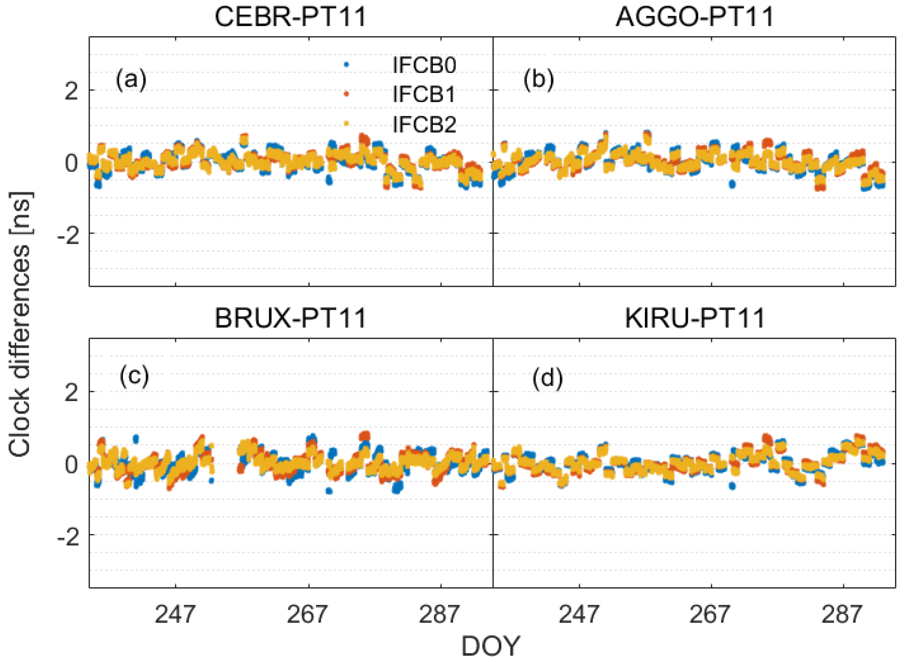
Figure 4 depicts the clock difference series of the stations equipped with the identical receivers (CEBR-PT11 and AGGO-PT11) or mixed receivers (BRUX-PT11 and KIRU-PT11). For convenience, the clock difference series has deducted the mean values. We can see that Figure 4 illustrates the good performance of time transfer when considering IFCB parameters, especially for IFCB2 schemes. We further support this finding by showing more results. 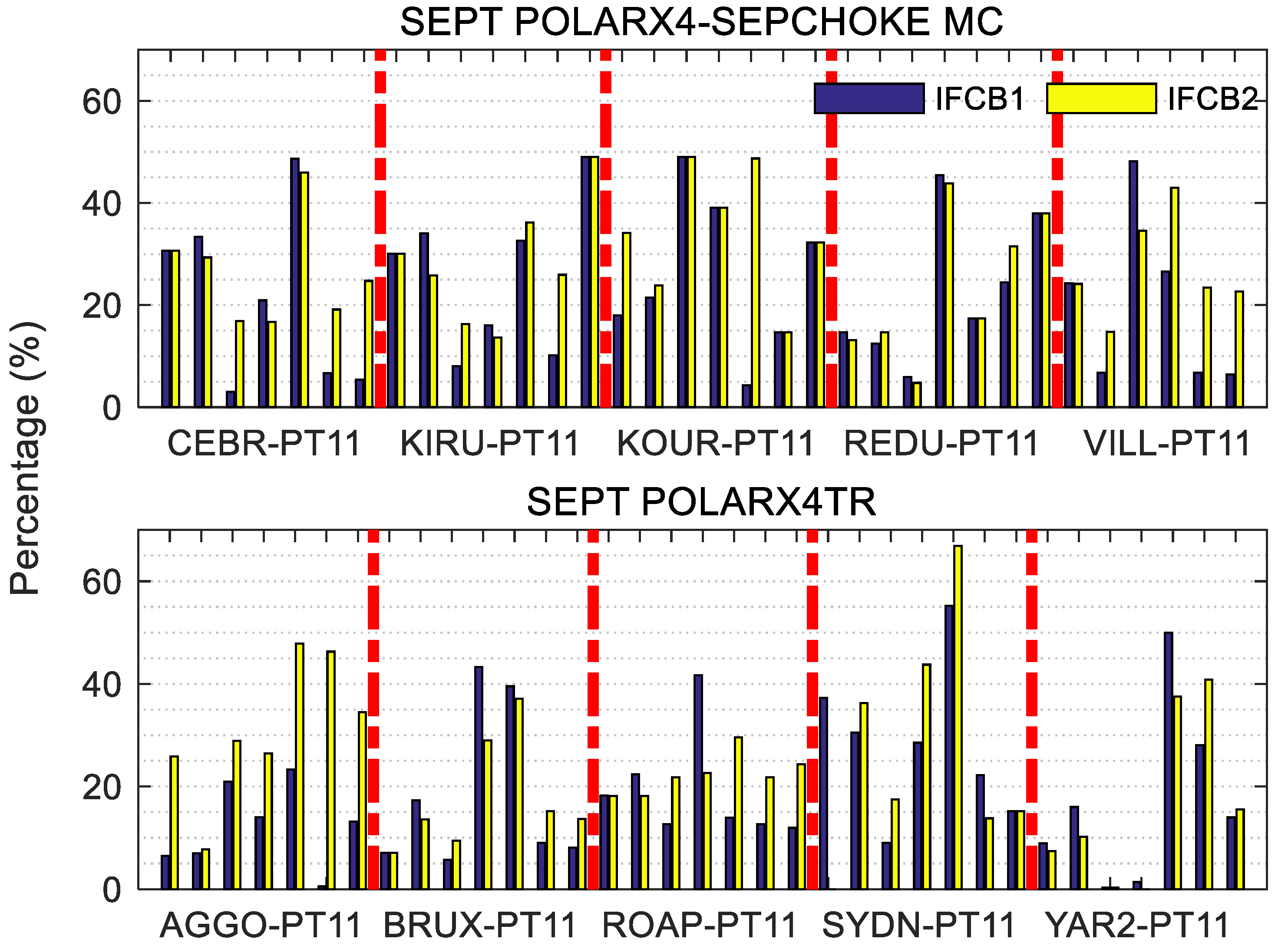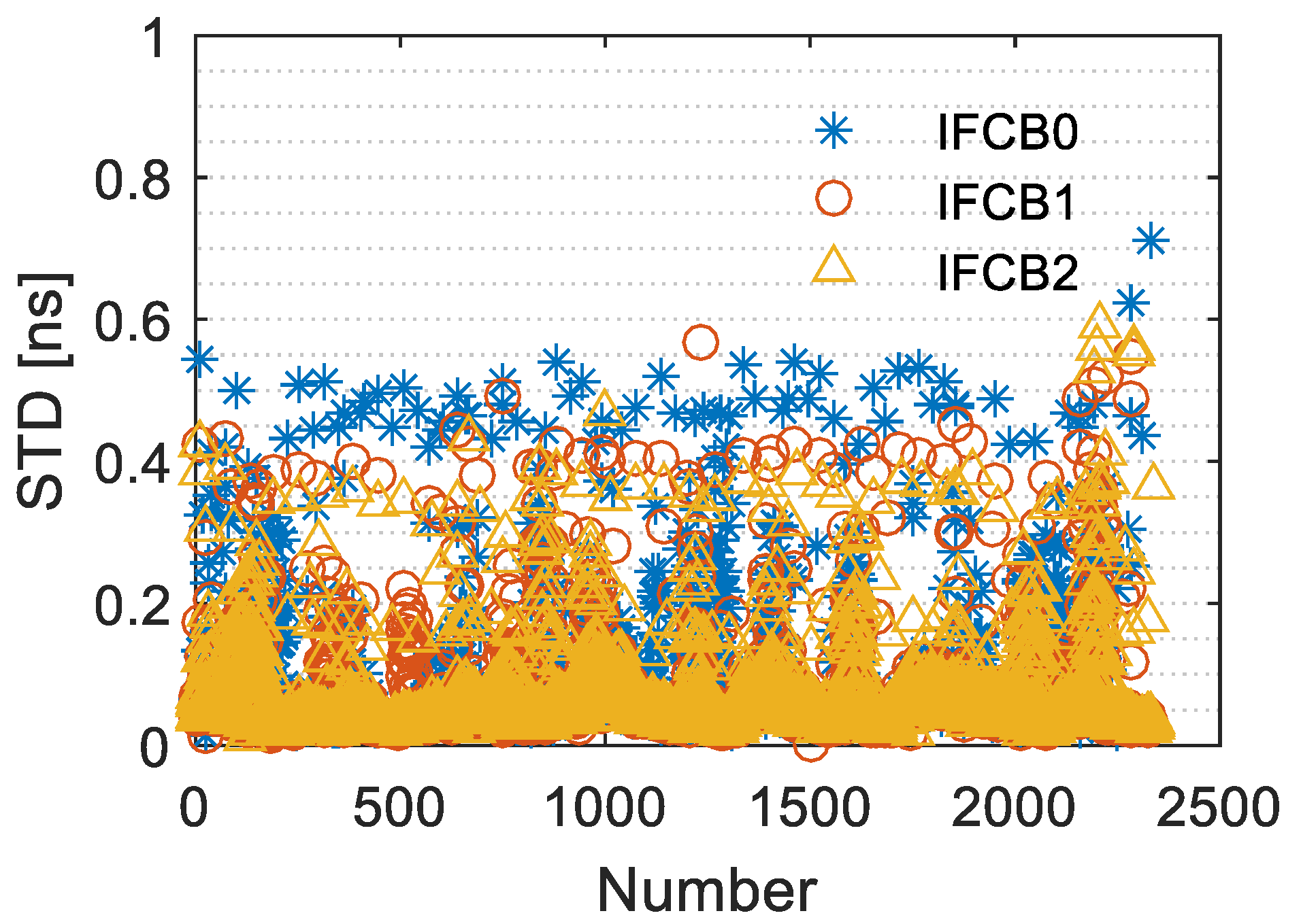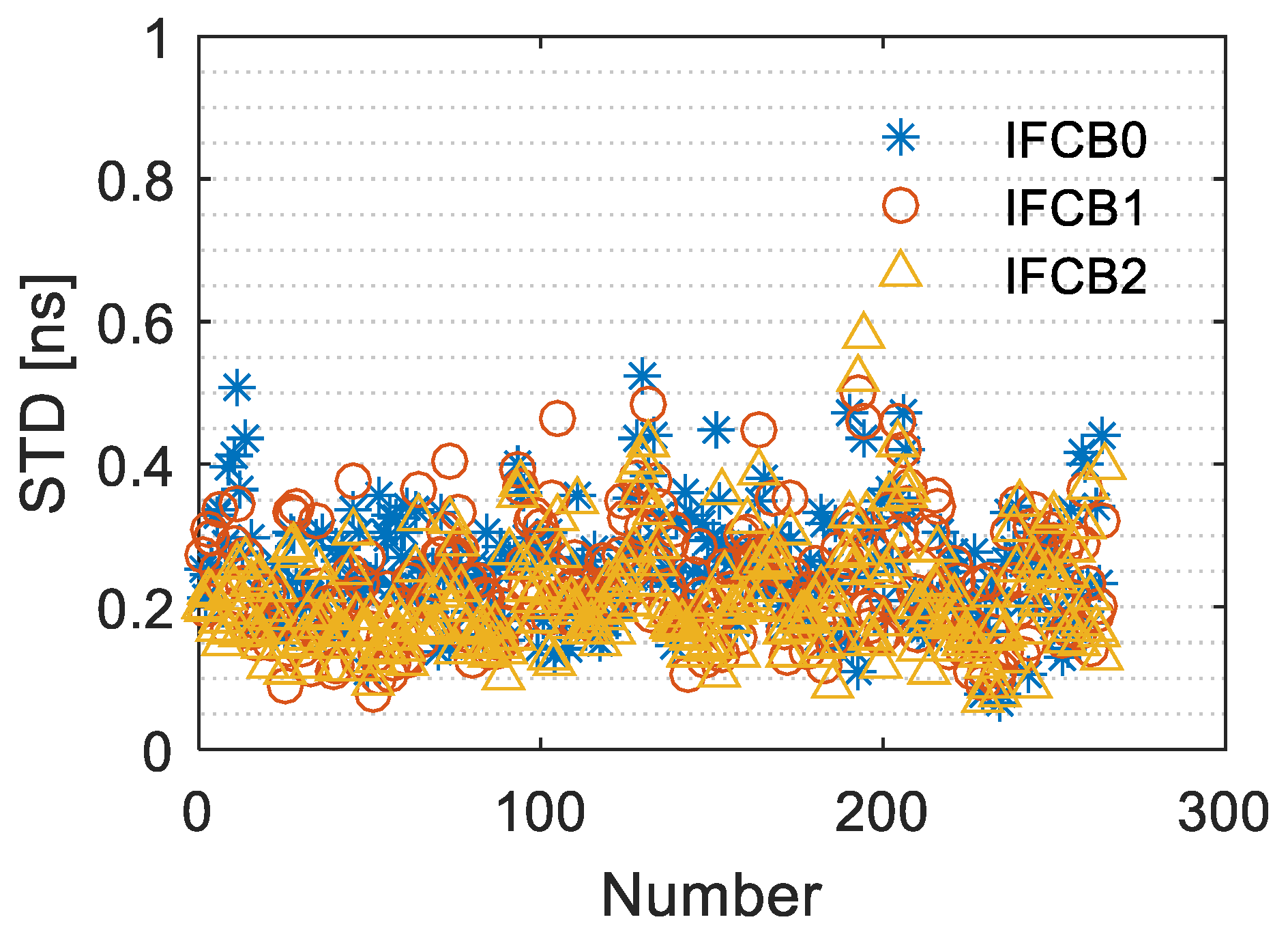Figure 5 shows the STD of the clock differences from the selected stations equipped with identical receivers (top) (CEBR-PT11, KIRU-PT11, KOUR-PT11, REDU-PT11 and VILL-PT11) and mixed receivers (bottom) (AGGO-PT11, BRUX-PT11, ROAP-PT11, SYDN-PT11 and YAR2-PT11), for the IFCB0, IFCB1 and IFCB2 solutions, respectively. Meanwhile, the uncertainty (STD) improvement of the IFCB1 and IFCB2 solutions are described in Figure 6. It is noted that the centre node, PT11, is equipped with SEPT POLARX4TR receiver and LEIAR25.R4 LEIT antenna. Taken together, we make three remarks. First, we can see that the STDs of the clock differences reach about 0.2 ns for the stations equipped with identical receivers or mixed receivers. Second, considering IFCB parameters, it is of interest to find an obvious improvement in the uncertainty (STD) of the GLONASS PPP-based time transfer. Compared with IF0, the percentage of improvement ranged from 3.0% to 49.0% for IFCB2. In addition, a similar characteristic is derived after considering the IFCBs for different stations equipped with identical receivers. Moreover, even though both ends of the time-links equipped with identical receivers (see in Figure 5 (top)), GLONASS PPP can reach better performance when considering the IFCBs. Third, similar to the solutions of stations equipped with the identical receivers, IFCB0 performs worst in the time transfer performance, while IFCB2 performs best. The uncertainty improvement is in the range of 0.96% to 59.4% and of 3.3% to 62.6% for the IFCB1 and IFCB2 solutions of the selected stations equipped with mixed receivers, respectively.

4.3. GLONASS PPP for Different End Users

In this part, the solutions of GLONASS PPP, neglecting the type of receiver and antenna, are presented by using CODE products. Furthermore, the coordinates of receiver of time-keeping laboratories are known values, while the coordinates of time users are unknown. Hence, the influence of IFCBs on GLONASS PPP-based time transfer for different end users (with/without fixing coordinates) are compared.

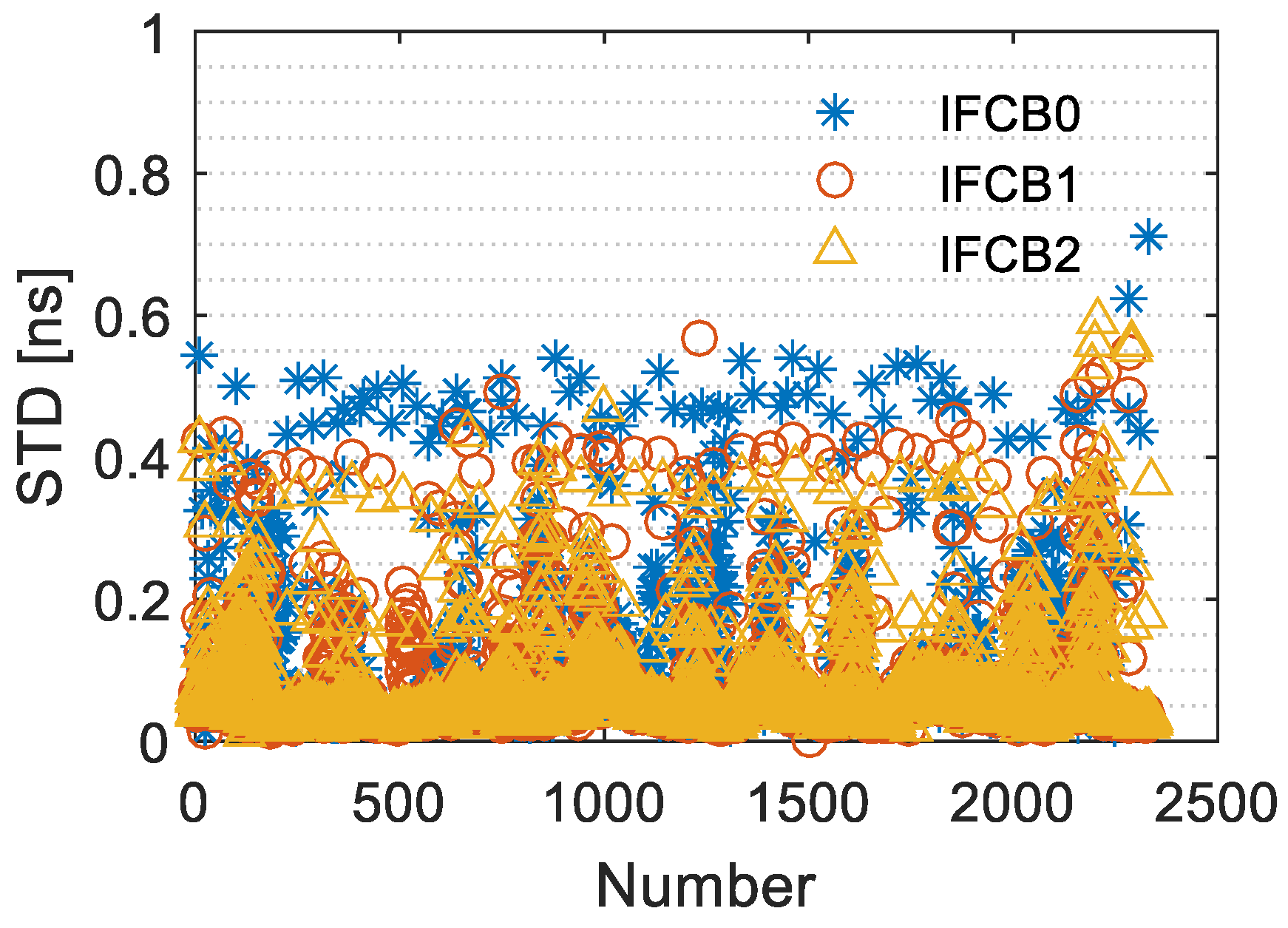
Figure 7 and Figure 8 display the STD series of one-day arc solutions and ten-day arc solutions, respectively, in different schemes with coordinate-fixed over all the tests. We can see that the STDs of the one-day arc solutions are mainly less than 0.2 ns, while a part of the solutions is poor. This result is, unexpectedly, the facts listed as follows. Figure 9 depicts the clock differences of AGGO-PT11 and BRUX-PT11 at DOY 235, 2017. Obviously, a clock discontinuity may be present at DOY 235 on two time-links. We address this issue by considering a representative example (depicted in Figure 10), which lost part of the observations depicted in the red box. The ambiguities will be re-estimated in the second arc. Hence, the solutions of GLONASS PPP present a clock discontinuity, while the GPS PPP shows a good performance due to the greater visibility of satellites. One the other hand, the STD of the 10-day solutions ranged from 0.1–0.4 ns. We further find that some results are greater than 0.4 ns, such as the TSK2-PT11 and STK2-PT11 time-links. We surmise that this may be related to the Geometric Dilution of Precision (GDOP). Zhou et al. [13] displayed the average global GDOP of GLONASS with an elevation cut-off angle of 7°. The results demonstrated that the GLONASS GDOP is analogous in the middle- and high-latitude regions than that in the low-latitude regions. Combined with Figure 7 and Figure 8, we can conclude that the day-boundary discontinuities are still a problem for GLONASS PPP-based time transfer. Meanwhile, the STDs of the clock difference were determined with one-day arc solutions and ten-day arc solutions in

Table 6. The uncertainty (STD) of the GLONASS PPP solutions with fixed coordinates (ns).

	The STD of One-Day Arc Solution (ns)		The STD of Ten-Day Arc Solution (ns)
	(95%)	(68%)	(95%)	(68%)
IFCB0	0.300	0.075	0.403	0.280
IFCB1	0.226	0.064	0.369	0.262
IFCB2	0.206	0.062	0.359	0.224

. We can observe that the 0.075 and 0.280 ns were obtained for the IFCB0 solutions at the 68% level in one-day arc solutions and ten-day arc solutions, respectively, while 0.300 and 0.403 ns at the 95% level, respectively. Interestingly, it is found that the STDs of the clock difference between the 68% and 95% levels for one-day solutions are slightly different. The difference can be attributed to the fact that the clock jumps due to the observation interruption. After considering IFCBs in GLONASS-only PPP, time transfer performance is improved compared to that of IFCB0. We further support this finding as shown in Table 6, which demonstrates that IFCB1 performs better than IFCB0, while IFCB3 performs best among the processing schemes. Taken together, uncertainty (STD) of IFCB2 is significantly improved by 30.0% from 0.300 to 0.211 ns and by 10.9% from 0.403 to 0.359 ns for the one-day arc solutions and ten-day solutions, respectively, at the 95% level. At the 68% level, the STD of the clock difference is significantly reduced, by 17.3% from 0.075 to 0.062 ns and by 20.0% from 0.28 to 0.224 ns for the one-day arc solutions and 10-day solutions, respectively. Moreover, we further find that the improvement in STD at the 95% level is more obvious than that at the 68% level for one-day arc solutions. As stated before, one can conclude that a good performance for GLONASS PPP can be achieved under the observation interruption when considering the IFCBs.

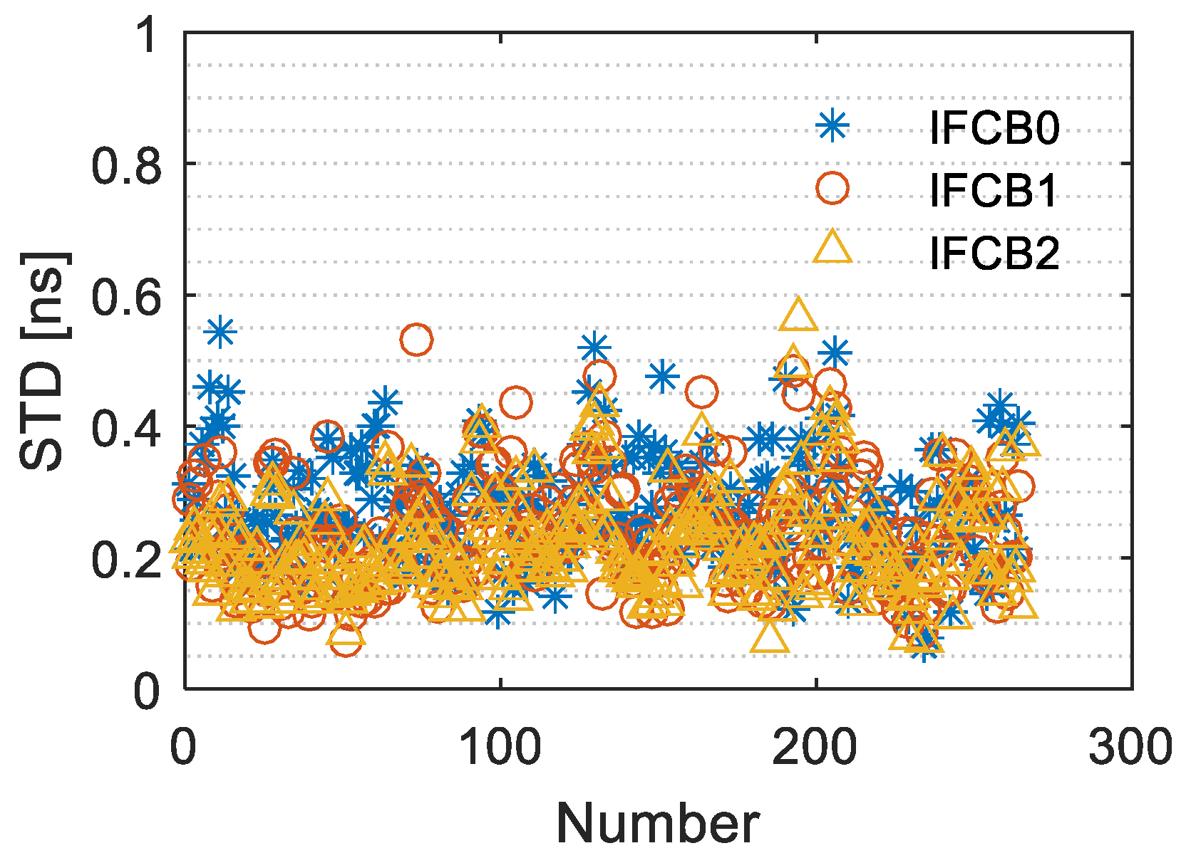
Usually, the coordinates of the receivers located in the time keeping laboratory are known values. Unlike the time keeping laboratory, they may be regarded as estimation parameters for the time users. To assess the influence of the IFCBs on the GLONASS PPP without coordinate-fixed, the STDs of the series of the one-day and ten-day arc solutions in different schemes are depicted in Figure 11 and Figure 12, respectively, without coordinate-fixed.

Table 7. The uncertainty (STD) of the GLONASS PPP solutions without fixed coordinates (ns).

	The STD of One-Day Arc Solution (ns)		The STD of Ten-Day Arc Solution (ns)
	(95%)	(68%)	(95%)	(68%)
IFCB0	0.304	0.074	0.411	0.305
IFCB1	0.230	0.065	0.369	0.272
IFCB2	0.211	0.064	0.368	0.236

presents the STDs of the GLONASS PPP at the 95 and 68% levels for the one-day and ten-day arc solutions, respectively. Similar to the GLONASS PPP with coordinate-fixed, the IFCB2 performs best. Compared with IFCB0, the STD of IFCB2 is reduced by 30.59% going from 0.304 to 0.211 ns, and by 10.46% going from 0.411 to 0.368 ns in one-day arc solutions and ten-day arc solutions at the 95% level, respectively. Besides, the different users (with and without coordinates fixed) are to be the same level. It is of great interest found that the improvement of the IFCBs is not obvious in the one-day arc solutions at the 68% level. We take this fact as an indication that the STDs of one-day arc solutions mainly depend on the accuracy of carrier phase observations. We further found that the STD of 10-day arc solutions is more notably improved at the 68% level than at the 95% level. This is not unexpected given that few bad results are obtained when considering IFCBs, and we do not attempt to cover all of them; rather, without a loss of generality and for the sake of clarity, the bad results have been depicted in Figure 8 and Figure 12. In the 266 tests of 10-arc solutions, there are 34 and 10 bad results for IFCB1 and IFCB2, respectively. These results further demonstrate that IFCB2 performs best.

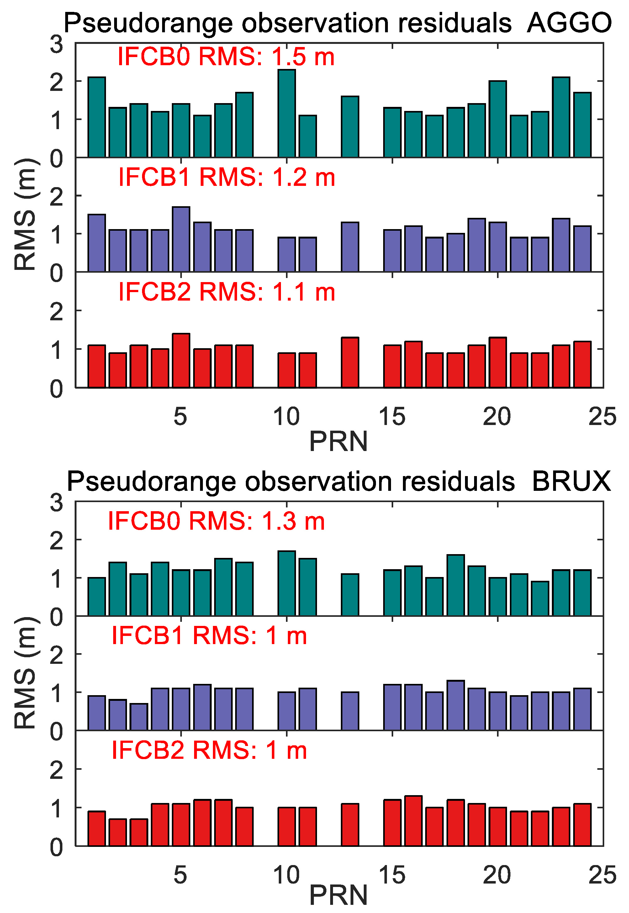
Since observation residuals contain measurement noise and other unmodeled errors, they can be used as important indicators to evaluate the PPP model. The pseudorange observation residuals at the two selected IGS stations (AGGO and BRUX) for the GLONASS PPP processing on DOY 227, 2017, are depicted in Figure 13. In the figure, the RMS statistics of each satellite in the different schemes are displayed in each panel. Neglecting GLONASS IFCB, larger RMS values can be observed, compared to the pseudorange residuals of IFCB1 and IFCB2. Overall, the statistical results clearly demonstrate that IFCB2 has the smallest proper handled in the IFCB2 model.

4.4. GLONASS PPP with Different IGS ACs Products

In this subsection, the performances of the GLONASS PPPs with different IGS ACs products are investigated for different IFCB handling schemes. Note that the GLONASS PPP solutions without coordinate-fixed are indicated herein.

Figure 14 shows the clock difference series of the two selected time-links using ESA and GFZ products in different schemes, respectively. The STD of the clock difference using the ESA and GFZ products at the 95 and 68% levels in the one-day arc solutions and ten-day arc solutions, respectively, are presented in

Table 8. The uncertainty (STD) of the GLONASS PPP solutions using ESA products with fixed coordinates (ns).

	The STD of One-Day Arc Solution (ns)		The STD of Ten-Day Arc Solution (ns)
	(95%)	(68%)	(95%)	(68%)
IFCB0	0.343	0.062	0.516	0.376
IFCB1	0.250	0.056	0.381	0.250
IFCB2	0.210	0.055	0.346	0.219

and

Table 9. The uncertainty (STD) of the GLONASS PPP solutions using German Research Center for Geosciences (GFZ) products with fixed coordinates (ns).

	The STD of One-Day Arc Solution (ns)		The STD of Ten-Day Arc Solution (ns)
	(95%)	(68%)	(95%)	(68%)
IFCB0	0.294	0.078	0.430	0.274
IFCB1	0.225	0.056	0376	0.253
IFCB2	0.203	0.054	0.366	0.213

. Taking Table 7, Table 8 and Table 9 together, it can be seen that the STD of the clock difference can be significantly reduced, especially for the ten-day arc solutions, when considering the GLONASS IFCBs. Interestingly, IFCB0 performs worst at the 95% and 68% levels, while IFCB2 performs best, even though different IFCBs processing strategies were adopted for different IGS ACs. This may be caused by the fact that when considering IFCBs at IGS ACs for each clock product that does not contain IFCBs, while IFCBs still exist in the pseudorange observations. This result means that IFCB estimation is necessary for the end user. Furthermore, estimating the IFCBs for each GLONASS satellite is the best choice. After applying the GFZ products, compared with IFCB0, the STD of IFCB2 is reduced by 23.47% from 0.294 to 0.203 ns, and by 14.88% from 0.430 to 0.366 ns, in the one-day arc solutions and ten-day arc solutions at the 95% level, respectively. At the 68% level, STD of IFCB2 is significantly reduced by 30.77% from 0.078 to 0.054 ns, and by 22.26% from 0.274 to 0.213 ns, for the one-day arc solutions and ten-day arc solutions, respectively.

The STD of the clock difference using the ESA products at the 95 and 68% levels in the one-day arc solutions and ten-day arc solutions, respectively, are depicted in Table 8. Taking Table 6, Table 8 and Table 9, it is of interest to note that different STD values of the clock difference are presented using different products. This difference can be attributed to the different accuracy of the precise orbits and clock for the IGS ACs. Similar to GLONASS PPP using the GFZ products, the IFCB2 schemes shows the best performance. Compared with IFCB0, the STD of IFCB2 is reduced by 38.78% from 0.343 to 0.210 ns, and by 32.95% from 0.516 to 0.346 ns in the one-day arc solutions and 10-day arc solutions at the 95% level, respectively. At the 68% level, STD of IFCB2 is obviously reduced by 11.29%, from 0.062 to 0.055 ns, and by 41.76%, from 0.376 to 0.219 ns for the one-day arc solutions and 10-day arc solutions, respectively.

5. Conclusions

In our work, GLONASS inter-frequency code biases (IFCBs) for GLONASS PPP-based international time transfer is modeled through a reparameterization process. Three different GLONASS IFCB handling schemes, which neglect IFCBs (IFCB0), estimate IFCBs for each GLONASS frequency number (IFCB1), and estimate each GLONASS satellite (IFCB2), were proposed for ionosphere-free GLONASS-only PPP. Seventy days of observation data from DOY 227–297 in 2017 from 36 stations of IGS network and three stations of time a keeping laboratory were selected to assess the model, and preliminary international time transfer results have been concluded. For the comparison, the GPS-only PPP solutions using IGS final products are regarded as reference. Clock differences between GPS- and GLONASS-only PPP solutions are then analyzed.

The quality of the IFCBs estimated for IFCB1 and IFCB2 are not equal. The bias is approximately 0.5 ns. The numerical results showed that for GLONASS PPP, considering the IFCBs can significantly reduce the STD of the clock difference for identical receivers (the reductions from 3.0% to 49%) or mixed receivers (the reductions from 3.3% to 62.6%). IFCB0 performs worst in the time transfer performance, while IFCB2 performs best for identical receivers or mixed receivers. Furthermore, the uncertainty (STD) of different end users, which include the exact coordinate of the station as known and unknown values, for example, time keeping laboratories and time users, shown a similar characteristic. Compared with neglecting IFCBs, the STDs of end users with coordinate-fixed were reduced by more than 30% from 0.3 to 0.2 ns, and 10% from 0.40 to 0.35 ns, at the one-day arc solutions and ten-days arc solutions, respectively, when estimating the IFCBs for each GLONASS satellite. The STDs of end users without coordinate-fixed improved by 30.59% going from 0.304 to 0.211 ns, and by 10.46% going from 0.411 to 0.368 ns in one-day arc solutions and ten-day arc solutions at the 95% level, respectively. Moreover, different precise products from the three IGS ACs were adopted for analysis. Even though different IFCBs handling strategies were adopted during their GLONASS satellite clock estimation, our numerical analysis showed that GLONASS-only PPP-based international time transfer achieved better performance when estimating IFCBs for each GLONASS satellite among using the three GLONASS final products.

Generally, estimating the IFCBs for each GLONASS satellite is superior for GLONASS PPP time transfer uncertainty improvement. The results suggest that, GLONASS IFCBs may not be strict for each satellite frequency. Therefore, it is recommended that this scheme can be utilized to handle GLONASS IFCBs in the PPP international time transfer processing for GLONASS observations.