1. Introduction
A broad range of experimental scientific fields have moved over the last few years from the study of scalar or vectorial quantities (i.e., measurement of a magnitude or a string of data as a function of a relevant variable) to the acquisition of images (i.e., 2D sets of data). The broad availability of cheap charge-coupled devices (CCD), the larger storage capabilities and the faster communication protocols have contributed to this remarkable change. In particular, in the field of Atomic and Molecular Physics, traditional methods, such as time-of-flight detection of ions or photoelectrons, are increasingly being replaced by techniques like ion or photoelectron imaging, or even ion–photoelectron coincidence imaging, for the study of photoionization, photodissociation, reaction dynamics or molecular alignment [
1,
2,
3,
4,
5,
6,
7,
8]. The acquisition of spatially-resolved data on the final position of these particles can yield a wealth of information of the process under study that was unimaginable with previous methods. In the analysis of these data, it has been common practice to analyze either integrated sections or cuts of the images to obtain 1D information that is then analyzed with standard 0D or 1D fitting procedures [
9,
10,
11,
12]. In many cases, the richness of the information that can be extracted from the data is lost. Multidimensional analysis can separate certain contributions that are often the key to unravel the dynamical processes.
In this work, we present a multidimensional fitting solution dedicated to obtain the best fit to the complete set of data contained in a time sequence of a sequence of velocity map images measured in femtosecond pump–probe experiments, through parameterized functionals that describe radial and angular properties of the particle distribution as a function of time. As will be shown, the multidimensional fit becomes essential for instance when contributions with different time behavior are overlapping. Additionally, for those cases where the initial guesses for the parameters or functional forms of the fit are misguided (on the number or nature of the contributions to the image, on the time behavior of anisotropy, etc...), discrepancies can be detected easily through the use of the analysis of the residuals. It is important to note that the multidimensional nature of the fit allows the discrimination of the different contributions to the images, in a manner that a reduced-dimensionality analysis cannot achieve. This method has revealed its value in a number of contributions where the need for discrimination of overlapping contributions in charged particle images was crucial [
13,
14,
15,
16,
17,
18]. The method is analogous to the global 2D fit approach used in Stolow’s group [
19,
20,
21,
22] but can easily be extended to extra dimensions such as the anisotropy, the temperature, the intensity dependence, measurements in coincidence, etc... With some modifications, the method can be equally applied to other problems, such as the detection of spectrally and spatially resolved X-rays from high-harmonic generation [
23], or temporal-spectral-spatial ultrashort pulse characterization [
24,
25,
26] and time-resolved time-of-flight measurements [
27]. For each particular application, functional shapes and dependences have to be adapted, but the strategy presented here is of general applicability to the study of 2D or higher dimensionality data. We describe the procedure in a pedagogical way to adapt any algorithms of optimization to a multidimensional analysis.
The paper is organized as follows. In
Section 2, the method to construct velocity map images and to describe their time evolution is presented, including both 3D and 2D versions. The multidimensional numerical fitting procedure is explained in
Section 3, and
Section 4 is dedicated to the application of the method to a case example: the femtosecond pump–probe velocity map imaging (VMI) experiment on CH
I predissociation on the
B-band.
Section 5 closes the paper with the main conclusions.
2. Construction of a Sequence of Velocity Map Images and Description of Its Time Evolution
The first demonstration of charged-particle imaging applied to reaction dynamics was made by Chandler and Houston. In their 1987 work [
1], they showed how it is possible to record, at once, the entire spatial distribution of fragments originating from a photodissociation event. In this way, within the resolution limits, it is possible to directly measure the angular and velocity distributions of the products of a chemical reaction. The technique of ion/photoelectron imaging made a giant leap a decade later with the discovery by Eppink and Parker of the technique that is known as velocity map imaging [
2], where through the use of open-lens electrodes with appropriate voltages, it is possible to work in a configuration where products of a photodissociation event with the same initial velocity vector are imaged onto the same position in the detector. This implies that the observed images are in fact 2D projections onto the plane of the detector of a velocity distribution on a spherical surface. Inversion techniques, such as the inverse Abel transform [
4,
28,
29,
30,
31], need to be implemented in order to extract the true distribution from the 2D projection. Further developments of this technique led to the discovery of slice imaging for ions [
32,
33,
34], where the extraction and detection conditions are such that only the central slice of the distribution on the sphere is detected, eliminating the need for inversion procedures that invariably introduce additional noise and required the existence of cylindrical symmetry in the interaction.
A typical image acquired in this type of experiment, either raw (through slice imaging), or, equivalently, mathematically inverted (through velocity map imaging), contains, in general, a set of “contributions” in the form of isotropic or anisotropic rings, by which we mean each of the possible processes or channels associated with a given ion or photoelectron. Typically, a “channel” is characterized by ions or photoelectrons with a given velocity (or center-of-mass kinetic energy) distribution, which, on the image, can be modeled, for instance, by a radial Gaussian function of the form
where
is the radial distance from the center of the image and
is the full-width-at-half-maximum (FWHM) of the contribution.
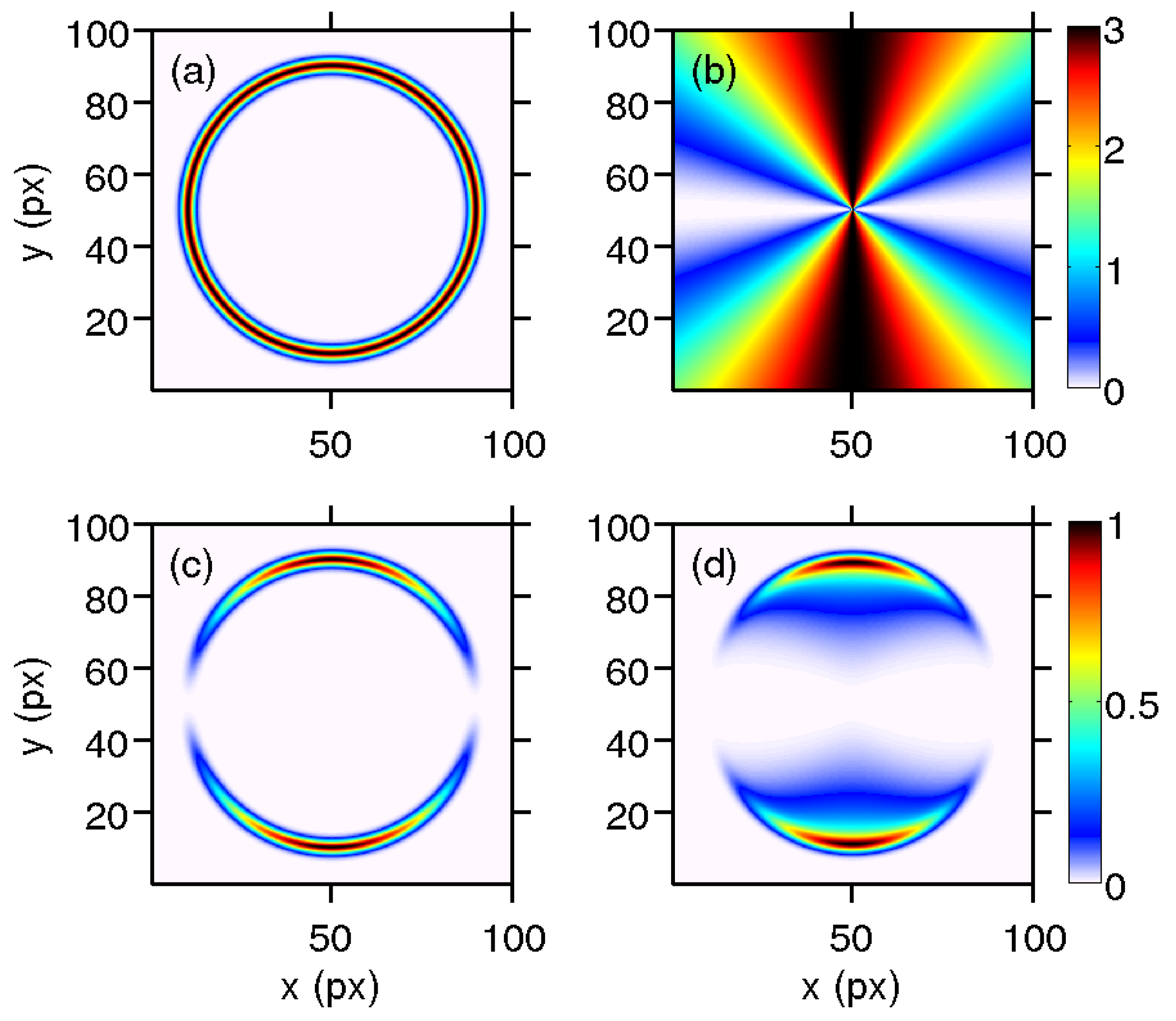
Figure 1a shows an example of such a contribution in the form of an isotropic ring with parameters
and
in units of pixels (px) of the CCD camera, which are proportional to the speed of the charged species.
The angular distribution (anisotropy) of charged particles for a given radius provides additional information on the nature of the channel. In the case of inversion symmetry, the anisotropy
A can be written as
where
is the angle between the polarization axis of the electric field and the considered direction and
n takes maximum values of 1 and 2 for one-photon and two-photon processes, respectively. Legendre polynomials,
, represent a complete angular basis set, which has the advantage that only few terms in Equation (
2) are generally sufficient to describe the ring anisotropy. A 2D plot of this function using
and
is shown in
Figure 1b.
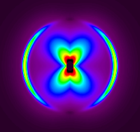
A channel can be fully described by the product of the velocity and angular distributions,
.
Figure 1c shows the result of the product of the 2D radial and angular representations shown in
Figure 1a,b.
The corresponding raw velocity map image can be simulated by applying the Abel projection [
4] and the result is shown in
Figure 1d. This simulation of a VMI image has been obtained assuming cylindrical symmetry on the 3D distribution, for which
Figure 1c is the central slice.
Multichannel processes lead to images
I with a collection of contributions
like the one described above. In the case that the different contributions do not interfere with each other, the experimental signal can be described by the following sum:
where
is the amplitude of each contribution. In the case that interferences occur, Equation (
3) would include additional interference terms.
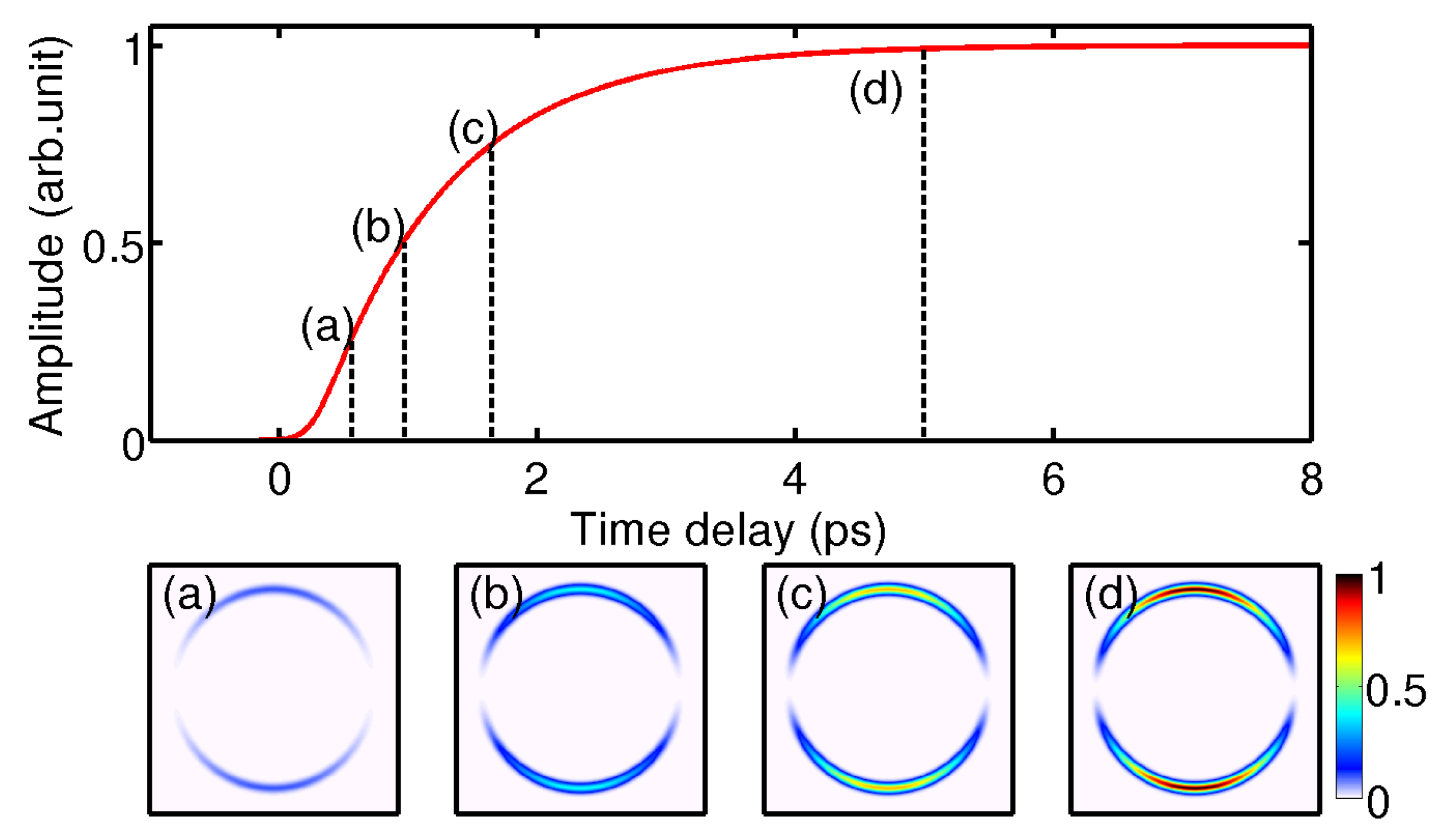
Let us now consider the particular case of a channel for which the shape of the velocity and angular distributions does not change with time. In that case, the temporal evolution
of the channel is represented just by an amplitude factor of the contribution that changes with time. For instance, in the case of a contribution which appears from the depopulation of an excited state (described by an exponential-type growth of the amplitude factor), the temporal behavior can be modeled as follows:
or in a more symbolic form,
where
is the Heaviside step function (for which
and
) and the temporal resolution corresponds to the cross-correlation between the two laser pulses
, modeled by a Gaussian function with a full width at half maximum of
, which is convoluted by the dynamics of the population of the state. The variable
represents the central pump–probe delay time for which the contribution appears, and
is the time constant of the exponential.
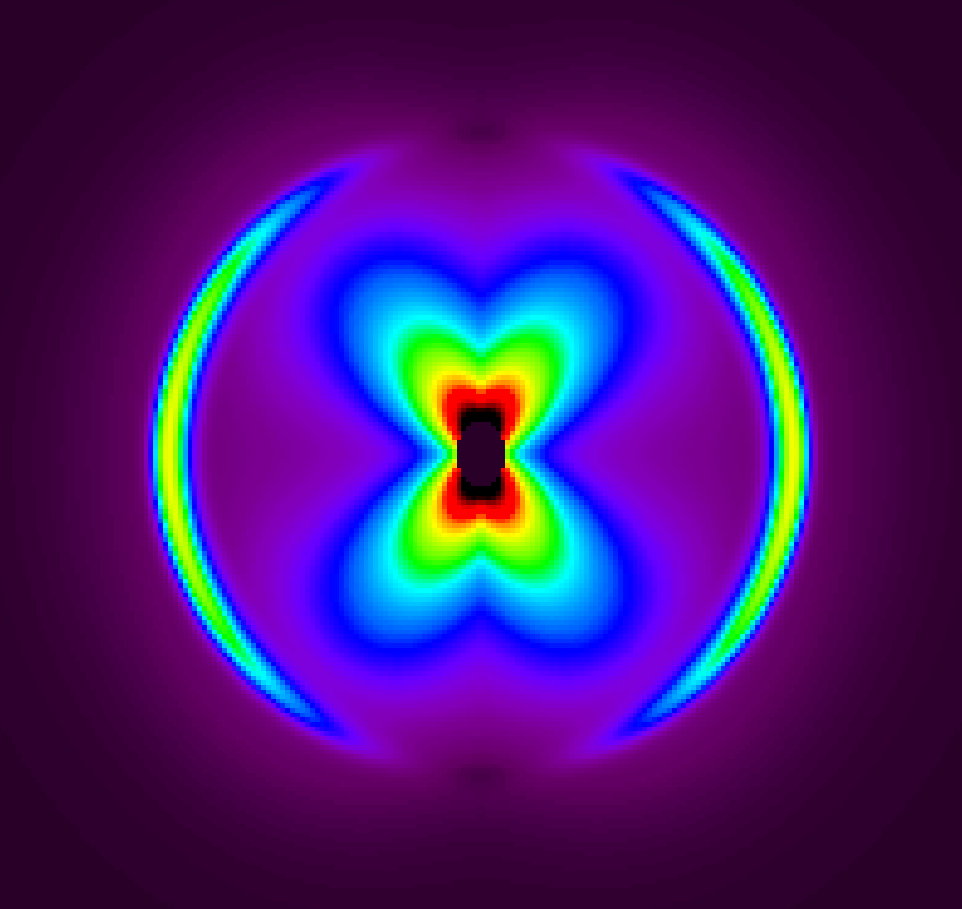
Therefore, the complete 3D description of a contribution
can be written as
This contribution is illustrated in
Figure 2.
In the particular case described above, time appears completely decorrelated from the other dimensions. However, in a more general case, some parameters of the radial or angular distributions can change with time. For example, the anisotropy can relax, the central position of the ring can shift or its width can vary. Hence, the contribution can be written in a more general way as:
where now both
R and
A become functions that depend on time. The
function could be contained in the functional form of
or
, but we have chosen to keep it explicitly written in Equation (
7) for convenience. This formalism can be generalized in a straightforward manner to any image scan as a function of an arbitrary observable, such as wavelength or temperature, for example, thus extending the dimensionality of the problem.
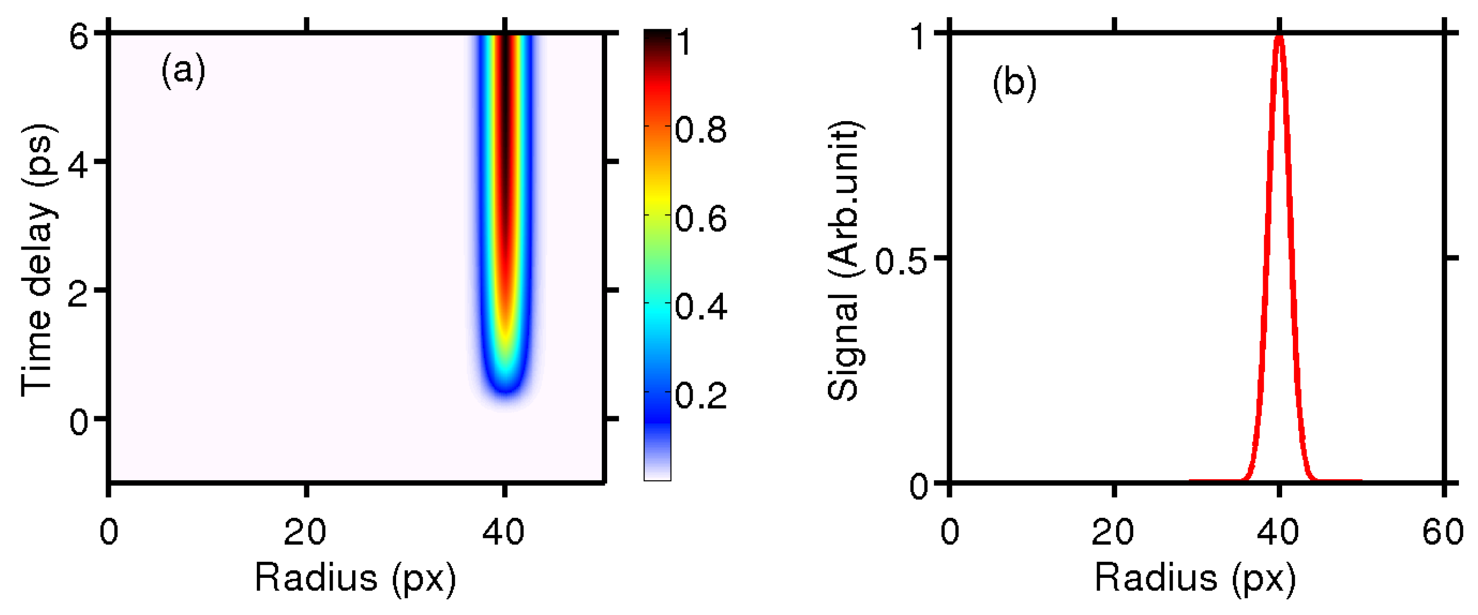
In some cases, the study of the dependence of the velocity distribution with time can be sufficient to extract all the relevant information of the pump–probe VMI experiment, with no additional insight to be gained from the anisotropy. In this situation, Equation (
7) can be angularly integrated and the signal originating from a given contribution becomes
in the case that the velocity distribution changes with time, or
if it does not.
A 2D representation (angularly integrated) of the contribution considered in
Figure 2 is displayed in
Figure 3a.
Figure 3b shows the velocity distribution (in pixels of the CCD camera) corresponding to a delay time of 5 ps. The amplitude and shape of the 2D and 3D representations can be directly compared through the angular integration
In the case that the non-zero anisotropy parameters
are limited to the first few orders, an alternative method to keep the 3D information consists of angularly integrating the VMI image in steps of
(10
for example) providing a set of 2D maps as follows:
In that case, the 3D fitting procedure is employed using the
n maps of
. This last method provides the same results as the direct 3D method (Equation (
7)) but tends to reduce the data size through the integration step. This can be employed in the case of slow convergence of the optimization algorithm.
3. Numerical Fitting Procedure
The quality of a 1D least-squares fitting procedure is related to the possibility to produce a 1D vector, constructed from a parameterized functional form, to fit a 1D data vector. The most commonly available fit procedures are developed for one dimension. Typically, the routine optimizes a set of parameters, , of a user-defined functional , which minimizes the global difference between the fit and the data for all values of the x variable.
A multidimensional fit can be performed using the same procedure by comparing each element of the matrix generated by the initial guess
with the corresponding element in the data matrix, and searching for a global minimization (in our case, the minimization algorithm employed is a Levenberg–Marquardt nonlinear regression method [
35,
36,
37]). In this sense, the multidimensional fit method can be performed using the standard 1D procedure for which all the elements of the
nD matrix are stored in a single 1D vector. In this approach, the multidimensional fitting procedure requires the use of invertible functions that convert an
n-dimensional matrix into a single vector. The method of choice is to construct a 1D vector that contains, in queue, all the columns of the matrix and all the images of the sequence. This same conversion procedure is applied to both simulated and data matrices before and after the use of the optimisation algorithm.
A second issue concerns the choice of coordinates. Whereas the formalism of
Section 2 is written in polar coordinates (
r, the distance from the center, and
, the angle from the vertical axis), the experimental signal is normally recorded using a widely available 2D CCD camera with pixels that are well defined in Cartesian coordinates. We propose relating the polar and Cartesian coordinates through the advantageous complex representation:
where (
) are the coordinates of the center of the image and
d is a distortion parameter of the image (different from unity in the case that the pixels are not square). In this way,
is defined from
to
with respect to the vertical-up semi-axis, which is taken as the origin angle. In the case that the polarization axis of the laser does not match with the vertical lines of the camera but holds an angle
with it, it can be taken into account by multiplying Equation (
12) by
. We choose to fix
in the singular case of
(i.e.,
and
are integers). The images shown in
Figure 1 and
Figure 2 are constructed using this conversion from polar to Cartesian coordinates.
As was mentioned before, it is common that VMI images are recorded as a function of an experimental variable of interest. Examples of this are pump–probe time delay, laser wavelength, polarization angle, temperature or sample density. This implies that a standard experiment performed in this way can produce tens or hundreds of images (for instance, pixels, with 12-bit dynamic range). With the conditions above, a single experiment with 100 images produces 50 MB in a stack of 3D data. Since the larger the size of the data stack, the slower the convergence of the minimization algorithm, it is important to find either symmetries or constraints that can reduce the number of data points. For example, in the case of symmetric Abel-inverted images, it is possible to work only with a square quarter of the image (corresponding to, say, pixels). The image size can be further reduced performing an () local integration, which reduces the size by a factor , although it can only be used if the spatial resolution required is not lower than n.
The description of a 3D functional necessarily requires a large number of parameters. The shape of each contribution along each axis and the correlations between them need to be considered. In the case of a time-resolved VMI experiment, the simplest contribution requires at least six parameters: one global amplitude, two temporal parameters (central position and time constant), two radial parameters (position and width) and one angular parameter (
in Equation (
2)). Indeed, the number of parameters increases with the number of observed channels. However, some parameters can be common for several contributions such as the origin of time which usually corresponds to the temporal overlap between the pulses and the width of some of the peaks that can be related to the apparatus function.
Initial guesses for the parameters must be carefully chosen in order to reduce the convergence time. A step by step procedure is proposed as follows. In order to find reasonable initial values for the parameters and test the functionals, prospective low resolution fits are previously carried out with an binning accompanied with a reduction of the number of images per time interval, so that the convergence time is reduced to a few minutes. The introduction of the contributions has to be performed stepwise, starting with the most intense one. A functional form for this main contribution is proposed, either empirically or from theoretical arguments, using parameters that can be estimated from visual inspection of a few images. Depending on the quality of the fit (looking at the residual), the functional can be improved. Then, the other contributions are introduced one by one using the same strategy. Finally, the final fitting is obtained by removing the binning and considering all the images.
4. Case Example: Analysis of a Femtosecond Pump-Probe VMI Experiment
In this section, we illustrate the strategy described in
Section 2 and
Section 3 to the analysis of an experimental image sequence obtained in a femtosecond pump–probe VMI experiment. We take as an example the photodissociation of CH
I in the
B-band, using a 201.2 nm femtosecond pump laser pulse where the appearance of the I*(
) fragment is probed by (2 + 1) resonance enhanced multiphoton ionization (REMPI) with an ultrashort 305 nm laser pulse [
38]. The dissociative mechanism of CH
I in the
B-band is relatively simple and consists of an electronic predissociation process [
39,
40,
41,
42]. The absorption of one pump photon at 201.2 nm excites the CH
I molecule from the electronic ground state into a bound Rydberg state in the ground vibrational state (
transition). This Rydberg state is crossed by a repulsive potential energy surface (PES) belonging to the
A-band, which correlates with CH
and I*(
) fragments [
43]. The initial population in the Rydberg state can be transferred into the repulsive PES with an efficiency that depends on the coupling between the two surfaces. Once the transfer is done, the dissociation of the molecule occurs in tens of femtoseconds producing CH
and I*(
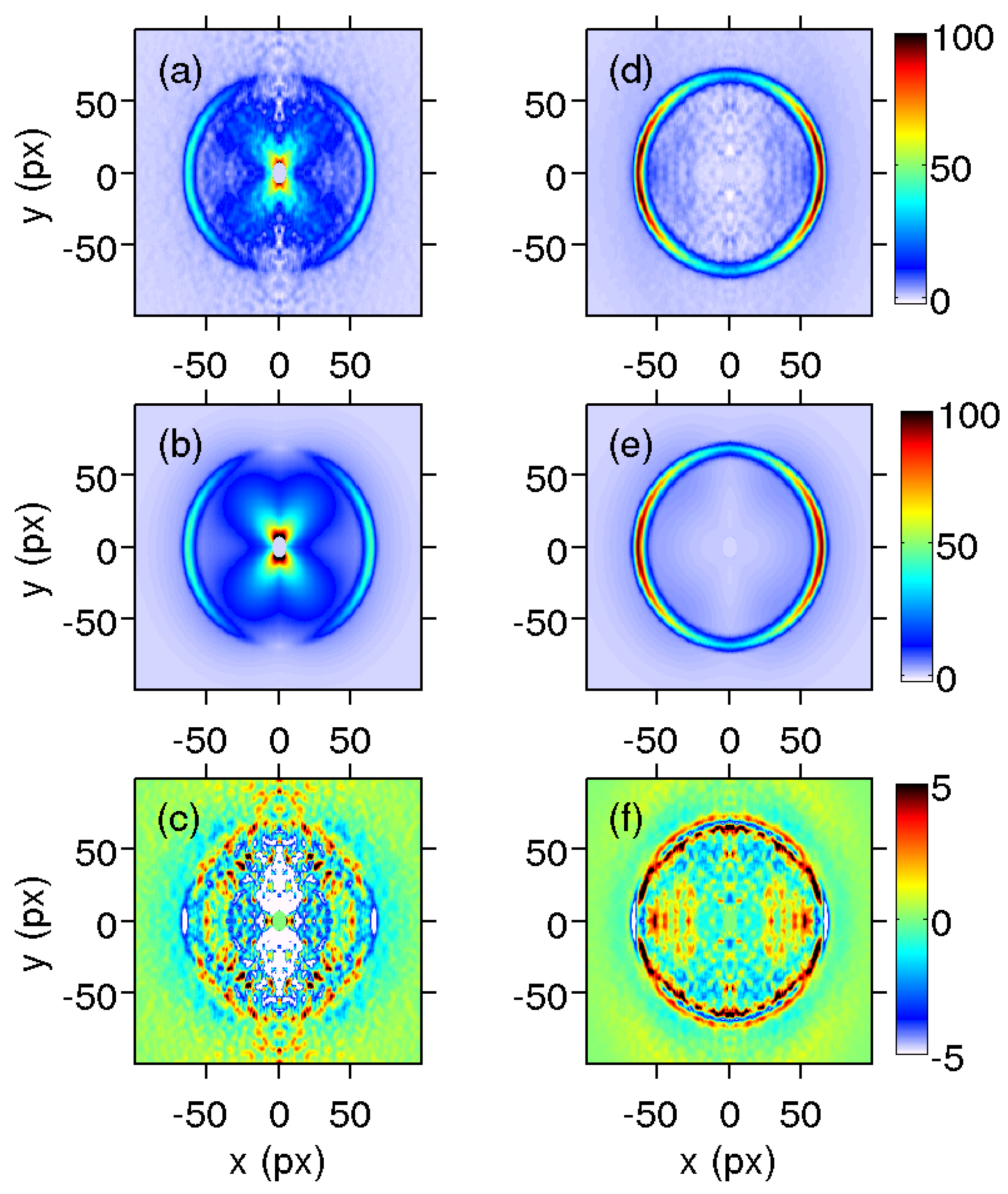
). When the iodine atom is created, it can be resonantly ionized by the probe pulse using a (2 + 1) REMPI scheme. The ionized fragments are accelerated by an external static electric field and focalized onto a microchannel plate coupled with a phosphor screen. The VMI-image (i.e., the Abel projection of the Newton sphere) is then recorded by a 12-bit Peltier cooled CCD camera. A set of images is recorded as a function of the pump–probe delay time. Each image is numerically inverted using an Abel inversion procedure [
28] to retrieve the 3D velocity distribution of fragments as shown in
Figure 4a,c. See Ref. [
38] for further details.
As usual in VMI experiments, each image contains information about the fragment velocity and angular distributions. Typically, a number of well defined rings representing the velocity-angle distribution of given photodissociation channels can be observed in the images. In the present case, the time and anisotropy evolution of one ring is clearly observed in the sequence of images. The amplitude of the signal of the ring depends on the number of iodine ions that are detected. The width of this contribution directly depends on the rovibrational temperature of the initial molecule and that of the CH
co-fragment, convoluted by the imaging apparatus resolution. The exact shape of the curve of the velocity distribution can be quite complicated; nevertheless, it can be reasonably approximated by Boltzmann, Gaussian or Lorentzian functions. In this experiment, the main ring can be modeled as the sum of two Gaussian functions, which represents the CH
co-fragment in the ground vibrational state (
) and with one quantum of vibrational excitation in the symmetric stretch mode (
). The temporal behavior expected for the relaxation of population can be modeled by an exponential function, as shown in Equation (
5). The anisotropy of a single linearly polarized photon phenomenon can be described by the second Legendre polynomial, considering
as the only non-zero coefficient in Equation (
2). The value of
primarily depends on the angular nature of the transition, i.e., whether the transition dipole moment is parallel or perpendicular to the dissociation axis. For the parallel case,
with a maximum value of
; for the perpendicular case,
with an extreme value of
. Both theoretical calculations and experiments for CH
I have shown that the transition from the electronic ground state to the
B-band is of perpendicular nature. The observed final anisotropy, measured through angular distributions of the fragments, can differ from the limiting cases of parallel (
) or perpendicular (
) anisotropy, mainly because rotation of the molecule prior to dissociation tends to blur the angular preference. This is especially relevant in the case of an indirect dissociation process if the time scales are similar or slower than molecular rotation.
Inspection of a few experimental images of the sequence shows that the anisotropy does evolve in this way [
38], i.e., images taken at earlier delay times show a more pronounced anisotropy than those taken at later times. The present example, therefore, provides a test of the fitting procedure where one of the angular parameters is a function of time. The functional form of the loss of anisotropy with time is not known. An exponentially decreasing modulus of the
parameter is proposed as:
where
is the asymptotic anisotropy parameter,
is the amplitude of the anisotropy parameter at
and
is the relaxation time. Some theoretical work has been dedicated to define the final value of
for a dissociation process that is either parallel or perpendicular, considering the dissociation time [
44,
45]. Those theoretical models are based on the rotation of the excited wave packet prior to dissociation. Although no predictions are available on the relaxation time, it can be estimated to be in the picosecond time scale.
The complete 3D function
that was employed to describe the main contribution (anisotropic ring) on the
B-band photodissociation of CH
I can be written as follows:
where
and
where two Gaussian functions describe the radial contributions corresponding to CH
fragments in the two vibrational states
and
, and with
representing the fraction of the population of CH
in
.
Femtosecond pump–probe VMI images contain, in general, some other low intensity secondary contributions, which can arise from different mechanisms, as, for example, absorption of two pump photons, relaxation of the molecule over another state which has lower absorption probability, detection by non-resonant ionization or background gas contamination. The secondary contributions have to be considered in the fitting procedure if they are overlapped with the contribution or contributions of interest. In fact, a good reproduction of the secondary signals allows the isolation of the contribution of interest from the rest by subtraction of the previously fitted secondary signals. If these secondary contributions are neglected, then an error is generated in the fit with a magnitude corresponding to the sum of the secondary signals in the spatial overlap region.
In the present case example [
38], the secondary contributions can be grouped into two classes. The first,
, appears in a broad range of velocities modeled by an asymmetric Gaussian function, i.e., with different widths (
and
) at each side of the maximum. It presents a
and
anisotropy. This contribution appears quickly at short delay times and then exponentially decreases with a constant time
. Due to a possible different number of photons involved, the temporal resolution
can be a priori different from the other contributions. The complete mathematical description can be expressed as follows:
with
and
The second minor contribution,
, has more localized velocities around the region of the contribution of interest (around
). Moreover, it has a temporal expression similar to
. Additionally, its anisotropy requires the consideration of both
and
constant terms. This last contribution is modeled by the following equations:
with
and
In what follows, the specific results of the 3D fitting procedure applied to the mentioned case example are presented.
Figure 4 shows two typical images, out of the sequence of 80 images recorded, fitted at short (120 fs) and asymptotic (10 ps) delay times.
In order to remove the standard 3–4 pixel region of noise produced by the Basex inversion around the central column of the images [
28], the fit has been carried out four pixels away from the central axis. Those points are thus removed from the fitted and measured images shown in
Figure 4. Additionally, some of the mathematical functions used in the fitting procedure present a singularity at the center of the images. In order to avoid the singularities, a 10 pixel circle was set to zero in the fitted and measured matrices. The elimination of these areas of the images does not represent any problem in the analysis, since all the relevant contributions are far away from the center.
The advantage of the 3D fitting procedure is that the anisotropy is considered. In the present case, the main contribution (ring) starts with a pronounced anisotropy (of perpendicular character), with the ion signal concentrated at the equator of the images, and later the ring evolves to become more isotropic. The anisotropy parameters of Equation (
16) obtained from the fit for this main contribution are
,
and
ps. Therefore, the fitted anisotropy at
is
, which is characteristic of a purely perpendicular transition.
The two secondary contributions are visible in the experimental images shown in
Figure 4. The first can be clearly seen at the center of the image shown in
Figure 4a; the second is appreciated at the vicinity of the main ring in
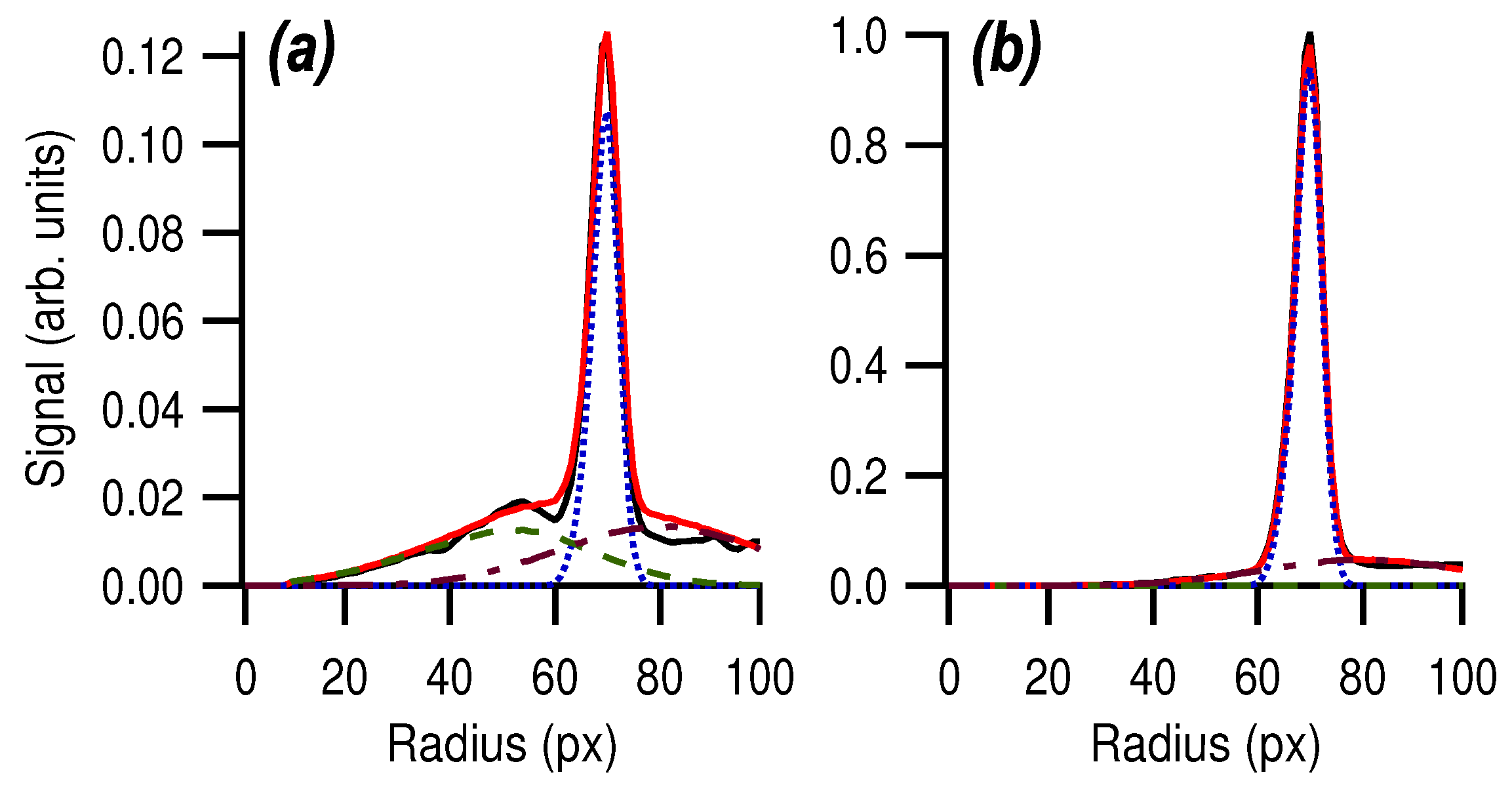
Figure 4d. These secondary contributions, together with the main contribution, can be distinguished in a more clear way in the velocity distributions shown in
Figure 5 at two delay times.
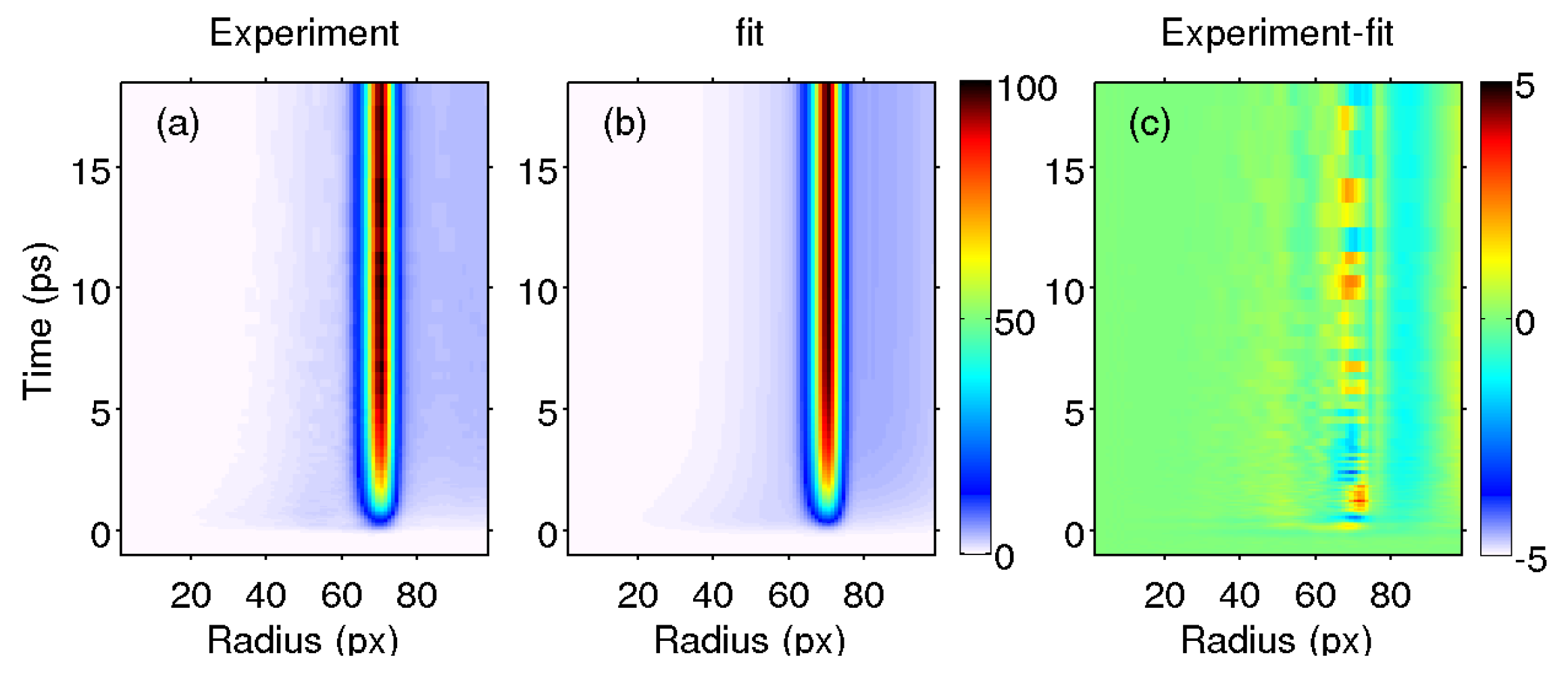
The time evolution of the velocity distribution can be well represented by angular integration of the images, as shown in
Figure 6.
The main contribution (ring) has been fitted in velocity (pixels) using the sum of two Gaussian functions, which have the same width (
pixel) as indicated in Ref. [
38]. The central position has been found to be at
px for the main peak and at
px for the minor shoulder with an amplitude
. As was indicated above, the main peak and the shoulder are assigned to dissociation channels yielding CH
and CH
(
), respectively.
The temporal evolution of the secondary contribution appearing in the center of the images has been fitted using a fs Gaussian convolution of a ps exponential decay. The other secondary contribution, , has a time constant of ps.
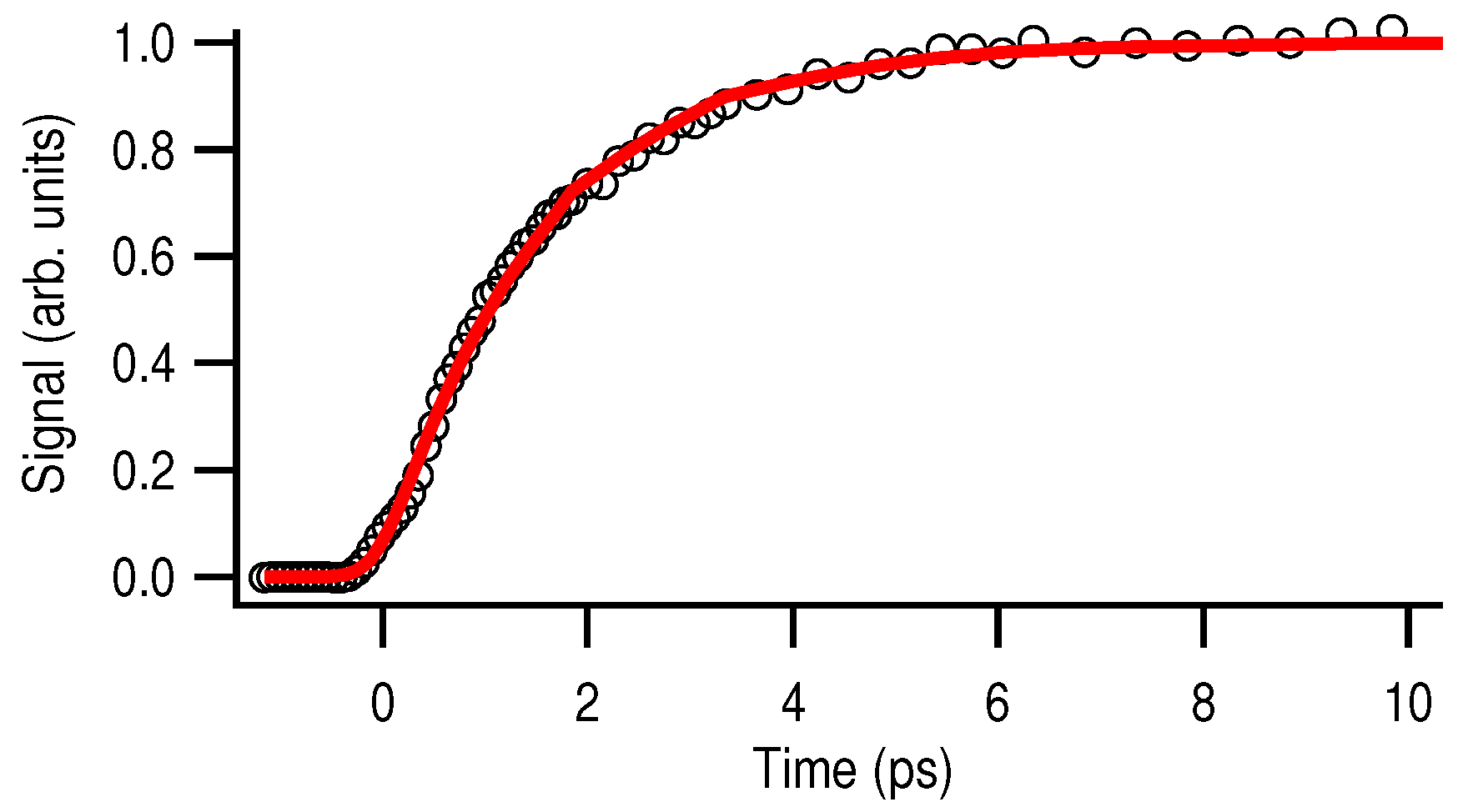
The temporal behavior of the contribution of interest
isolated from the secondary contributions is shown in
Figure 7 as a 1D transient. The data points shown in this figure have been obtained through subtraction of the fitted secondary contributions from the experimental measurement. Then, the resulting signal has been fully integrated angularly and radially integrated over the region of interest.
An exponential-type growth (Equation (
15)) with a time constant of
ps for this particular case has been found from the fit. Several (from 6 to around 30) independent sets of measurements across the full temporal range were acquired. Each time resolved-VMI measurement is independently fitted, keeping the same mathematical function. Each Levenberg–Marquardt fit provides fitting parameters and their corresponding standard deviations. A statistical study of the parameters that may not change with the scan, such as lifetimes of a given state, is hence performed. For such parameters, the extracted value is defined by the center of mass of the parameters found by each fitting procedure weighted by the inverse of its own standard deviation. Its respective error is hence the weighted dispersion of the individual values. The time constant thus obtained has been found to be
ps, as shown in Ref. [
38].
The computer time required for the fit strongly depends on the chosen algorithm (Levenberg–Marquardt, genetic algorithm, ...), the possibility of parallel the calculations, the computational language, the size of the data, the number of contributions involved in the process, the number of parameters required, the quality of estimation of the initial guess and many other parameters. As an indication of the fit described in this section, considering around 30 parameters, it takes only 1–2 min with an un-paralleled CPU and a computer with an Intel core i7-2700K CPU (Santa clara, CA, USA) at 3.5 GHz with 16 Go RAM Matlab (R2013a) (Mathworks, Natick, MA, USA) based program running on Debian operating system.


