Incorporating Grey Total Influence into Tolerance Rough Sets for Classification Problems

Abstract

Tolerance-rough-set-based classifiers (TRSCs) are known to operate effectively on real-valued attributes for classification problems. This involves creating a tolerance relation that is defined by a distance function to estimate proximity between any pair of patterns. To improve the classification performance of the TRSC, distance may not be an appropriate means of estimating similarity. As certain relations hold among the patterns, it is interesting to consider similarity from the perspective of these relations. Thus, this study uses grey relational analysis to identify direct influences by generating a total influence matrix to verify the interdependence among patterns. In particular, to maintain the balance between a direct and a total influence matrix, an aggregated influence matrix is proposed to form the basis for the proposed grey-total-influence-based tolerance rough set (GTI-TRS) for pattern classification. A real-valued genetic algorithm is designed to generate the grey tolerance class of a pattern to yield high classification accuracy. The results of experiments showed that the classification accuracy obtained by the proposed method was comparable to those obtained by other rough-set-based methods.

1. Introduction

Rough set theory [1,2] can effectively deal with the formulation of vague concepts [3,4,5,6,7,8,9,10]. Traditional rough-set-based methods use discretization methods to deal with quantitative attributes. Given that no one method of discretization is optimal, the tolerance rough set (TRS) has proven effective in dealing with problems involving numerical attributes [11,12,13]. Several TRS-based classifiers (TRSCs) use the traditional TRS with a simple distance measure to estimate similarity between any pair of patterns, viewing each category in a classification problem as a concept [11,12,13,14,15,16,17,18,19,20,21]. To expand the applicability of TRSCs, instead of the simple distance measure, several measures such as flows [22] and relationships [19,23] among patterns have been proposed to improve classification performance.

Direct relationships have been effectively measured in grey TRSC [19] through grey relational analysis (GRA) from the viewpoint of relationships obtained between patterns. However, direct as well as indirect relationships can exist between patterns. The widely used Decision-Making Trial and Evaluation Laboratory (DEMATEL) can effectively verify interdependencies among patterns or variables [20,21,22]. Furthermore, the total influence matrix plays an important role in the DEMATEL, and can be used to indicate direct/indirect influences among patterns. This is why the DEMATEL has been widely applied to various decision problems [24,25]. This motivated us to use the total influence matrix to realize direct/indirect relationships when constructing a TRS-based classifier. This article thus proposes a grey-total-influence-based TRS (GTI-TRS) for pattern classification. Furthermore, a genetic algorithm is used to determine the parameters required to construct the proposed classifier with high classification accuracy.

The remainder of this paper is organized as follows. Section 2 introduces a traditional similarity measure for the TRS and its computation steps. In Section 3, we present the proposed grey total influence matrix and GTI-TRS for pattern classification. In Section 4, we provide a genetic algorithm to construct the proposed GTI-TRS-based classifier (GTI-TRSC). Some real-world datasets were used to determine the classification accuracy of the proposed method. The experiments and results described in Section 5 show that the proposed GTI-TRSC can perform well compared to rough-set-based methods considered. Section 6 contains a discussion of the results and the conclusions of this study.

2. Tolerance Rough Sets

The rough set is briefly introduced in Section 2.1. TRS with a similarity measure is described in Section 2.2. In Section 2.3, we detail the classification procedure for the TRSC.

2.1. Rough Set Theory

Uncertainty and vagueness can be handled by rough set theory. Let S = (U, A ⋃ {d}) be a decision table, where U, A, and D are nonempty finite sets. U is the universe of objects, A is a set of conditional attributes, and d ∉ A is a decision attribute. An information function a: U → V_a can be defined for a ∊ A, where V_a is the set of values of a called the domain of a. An indiscernibility relation Ind(P) is defined for any P ⊆ A:

$$\mathrm{Ind}\left(P\right)=\{(x_i,x_j)\in U^2|a(x_i)=a(x_j),\forall a\in P\}$$

(1)

where x_i and x_j are indiscernible if (x_i, x_j) belongs to Ind(P). Ind(P) is called the P-indiscernibility relation, and its equivalence classes are denoted by [x]_P = {y ∊ U$|$a(x) = a(y), ∀a ∊ P}. A P-definable set denotes any finite union of elementary sets [26]. In a classification problem, a concept X is composed of elements with the same class label such that X ∊ U/{d}.

Sometimes, X ⊆ U is not P-definable. If X is a vague concept, a pair of precise concepts, P-upper ($\overline{P}$X) and P-lower approximations ($\underset{¯}{P}$X), can be used to approximate X [1,8]:

$$\overline{P}X=\left\{x\right|x\in U, {[x]}_P\cap X\ne \varphi \}$$

(2)

$$\underset{¯}{P}X=\left\{x\right|x\in U,{[x]}_P\subseteq X\}$$

(3)

It is clear that $\underset{¯}{P}$X ⊆ $\overline{P}$X. Elements that certainly belong to X constitute $\underset{¯}{P}$X, whereas those possibly belonging to X constitute $\overline{P}$X. The tuple 〈$\underset{¯}{P}$X, $\overline{P}$X〉 is called a rough set, and $\underset{¯}{P}$X and $\overline{P}$X are singleton approximations. When $\overline{P}$X = $\underset{¯}{P}$X, X is definable because X is precise with respect to P. In contrast, $\overline{P}$X ≠ $\underset{¯}{P}$X means that X is undefinable.

A boundary region BND_P(X) defined for a vague concept X is as follows:

$$BN{D}_P\left(X\right)=\overline{P}X-\underset{¯}{P}X$$

(4)

A rough membership function defines the degree of inclusion of x within X with respect to P:

$${\mu }_X^P(x) =\frac{\left|{[x]}_P\cap X\right|}{\left|{[x]}_P\right|}$$

(5)

where ${\mu }_X^P(x)$ ∊ [0, 1], and |[x]_P| denotes the cardinality of [x]_P.

2.2. Traditional Similarity Measure

Let m and n denote the numbers of patterns and attributes, respectively. x_i and x_j (1 ≤ i, j ≤ m) are some objects in U. A simple distance function can be defined by a similarity measure S_a(x_i, x_j) to measure the closeness between a(x_i) and a(x_j) as in [14,15]:

$$S_a(x_i,x_j) =1-\frac{\left|a(x_i)-a(x_j)\right|}{d_{max}}$$

(6)

where a(x_i) and a(x_j) are attribute values of x_i and x_j, respectively, in V_a, and d_max is the maximum value among |a(x_i) − a(x_j)|. d_max can be replaced by (max_a − min_a) [17], where max_a and min_a are the maximum and minimum values, respectively, of the domain interval of a [12]. Then, x_i and x_j are similar with respect to a when S_a(x_i, x_j) ≥ t_a, where t_a ∊ [0, 1] is the similarity threshold with respect to a. The tolerance relation R_a has a relation with S_a(x_i, x_j):

a(x_i) R_a a(x_j) ⇔ S_a(x_i, x_j) ≥ t_a

(7)

This means that x_i and x_j are similar with respect to attribute a when a(x_i)R_a a(x_j). S_A(x_i, x_j), an overall similarity measure, can be further defined as:

$$S_A(x_i,x_j) =\hspace{0.17em}\frac{{\displaystyle \sum _{a\in A}{S}_a}(x_i,x_j)}{\left|A\right|}$$

(8)

where |A| is the number of attributes in A, and |A| = n here. Kim and Bang [14] used x_i τ_A x_j to denote the above similarity between objects x_i and x_j with respect to all attributes A. As a result, the tolerance relation τ_A can be related to S_A as

x_i τ_A x_j⇔ S_A(x_i, x_j) ≥ t_A

(9)

where t_A ∊ [0, 1] is a similarity threshold based on A.

Patterns that have a tolerance relation with x_i form a tolerance class TC(x_i) of x_i:

TC(x_i) = {x_j∊ U|x_i τ_A x_j}

(10)

X can be approximated by the lower ($\underset{\_}{{\tau }_A}$X) and upper approximations ($\overline{{\tau }_A}$X). For subset approximations, $\underset{\_}{{\tau }_A}$X and $\overline{{\tau }_A}$X are defined as [26]:

$$\underset{\_}{{\tau }_A}X=\cup \left\{TC\left(x\right)\right|x\in U,TC\left(x\right)\subseteq X\}$$

(11)

$$\overline{{\tau }_A}X=\cup \left\{TC\left(x\right)\right|x\in U,TC\left(x\right)\cap X\ne \phi \}$$

(12)

For concept approximations, $\underset{\_}{{\tau }_A}$X and $\overline{{\tau }_A}$X are defined as:

$$\underset{\_}{{\tau }_A}X=\cup \left\{TC\left(x\right)\right|x\in X,TC\left(x\right)\subseteq X\}$$

(13)

$$\overline{{\tau }_A}X=\cup \left\{TC\left(x\right)\right|x\in X,TC\left(x\right)\cap X\ne \phi \}$$

(14)

The tuple 〈$\underset{\_}{{\tau }_A}$X, $\overline{{\tau }_A}$X〉 is the tolerance rough set. The main difference between these two approximations is associated with objects belonging to U or X.

2.3. Computational Steps of a TRS-Based Classifier

The computational steps of a TRSC [14,15] can be briefly described as follows:

Step 1.

Determine 〈$\underset{\_}{{\tau }_A}$TC(x), $\overline{{\tau }_A}$TC(x)〉

With x, $\underset{\_}{{\tau }_A}$TC(x) is composed of patterns certainly similar to x, and $\overline{{\tau }_A}$TC(x) is composed of patterns possibly similar to x. For subset and concept approximations, $\underset{\_}{{\tau }_A}$TC(x) is identical to TC(x), but $\overline{{\tau }_A}$TC(x) is not.

Step 2.

Classification using lower approximations

If $\underset{\_}{{\tau }_A}$TC(x) = {x}, the classification of x can be left to the next step. If the cardinality of $\underset{\_}{{\tau }_A}$TC(x) is at least two, $\underset{\_}{{\tau }_A}$TC(x) − {x} is used to determine the relative frequency of the class inclusion of the training patterns in $\underset{\_}{{\tau }_A}$TC(x) − {x}. Then, x can be assigned to the class with the highest relative frequency by majority vote. However, if the highest relative frequency is not unique, the classification of x can be left until the next step.

Step 3.

Classification using upper approximations

The boundary region BND_A(TC(x)) ($\overline{{\tau }_A}$TC(x) − $\underset{\_}{{\tau }_A}$TC(x)) of x can be used to determine the class label of x. Assume that patterns belonging to class C_i constitute X_i. With y in BND_A(TC(x)) ≠ φ, the rough membership function denoted by ${\mu }_{C_i}(y)$ defined as:

$${\mu }_{C_i}(y)\hspace{0.17em}=\hspace{0.17em}\frac{\left|TC(y)\cap X_i\right|}{\left|TC(y)\right|}$$

(15)

where |TC(y)| denotes the cardinality of TC(y). Then, the average rough membership function of x regarding C_i is computed as:

$${\overline{\mu }}_{C_i}(x)\hspace{0.17em}=\hspace{0.17em}\frac{1}{m}{\displaystyle \sum _{y\in {\mathrm{BND}}_A(\mathrm{TC}(x))}{\mu }_{C_i}(y)}$$

(16)

where m is the cardinality of BND_A(TC(x)). x can be assigned to a class with the largest degree of average rough membership. However, the class label of x cannot be confirmed if BND_A(TC(x)) = φ.

3. Grey-Total-Influence-Based Tolerance Rough Sets

The proposed GTI-TRS plays an important role in designing the proposed classifier. Thus, related studies with respect to the measurement of total influence are first described in Section 3.1. Three main components constitute the GTI-TRS: the GRA introduced in Section 3.2, the proposed grey total influence presented in Section 3.3, and the GTI-based tolerance relation described in Section 3.4.

3.1. Studies Related to Measuring Total Influence

Pattern classification refers to the problem of partitioning a pattern space into classes and assigning a pattern to one of them [15]. As mentioned above, to improve the classification performance of the TRSC, this study addresses direct relationships measured in the grey TRSC [19]. The main issue addressed is that as a pattern is likely to influence another directly and/or indirectly, indirect relationships among patterns should be studied as well. To develop novel similarity measures for the TRS by means of relationships, this study focuses on ways of leveraging direct relationships among patterns measured by GRA to further generate the total influence, consisting of indirect and direct relationships, for a TRSC. It should be noted that many studies (e.g., [19,27,28,29]) have shown the effectiveness of GRA in measuring relationships among attributes and patterns.

The use of grey theory to measure direct influences among patterns for the DEMATEL has been addressed in recent studies, such as [30,31,32,33,34,35,36]. These studies derived the total influence matrix by representing a direct influence as a grey number [27]. As the proposed method derives the total influence matrix by using GRA to automatically generate direct influences from crisp-valued data, the focus is completely different from that of the aforementioned grey DEMATEL methods.

3.2. Grey Relational Analysis

Unlike statistical correlation measuring the relationship between random variables, GRA explores relationships between data sequences [27,29] by treating one of these sequences as the goal [28]. Assume that n denotes the number of attributes. Let x_j = (x_j1, x_j2, …, x_jn) (1 ≤ j ≤ m) be a comparative sequence and x_i = (x_i1, x_i2, …, x_in) (1 ≤ i ≤ m) be a reference sequence. The grey relational coefficient ξ_k(x_i, x_j) can be used to measure the relationship between these two sequences on attribute k (1 ≤ k ≤ n) [37]:

$${\xi }_k\left(x_i,x_j\right) =\frac{{\Delta }_{\min }+\rho {\Delta }_{\max }}{{\Delta }_{ijk}+\rho {\Delta }_{\max }}$$

(17)

where

$${\Delta }_{min}=\underset{s}{\min }\hspace{0.17em}\underset{l}{\min }\hspace{0.17em}\left|x_{jl}–x_{sl}\right|, 1 \le s\le m, 1 \le l\le n$$

(18)

$${\Delta }_{\max }=\underset{s}{\max }\hspace{0.17em}\underset{l}{\max }\hspace{0.17em}\left|x_{jl}–x_{sl}\right|, 1 \le s\le m, 1 \le l\le n$$

(19)

Δ_ijk = |x_ik − x_jk|

(20)

where ρ is a discriminative coefficient, commonly specified as 0.5 [29], but this is apparently not an optimal setting. ξ_k(x_i, x_j) falls somewhere between zero and one.

The grey relational grade (GRG) ϒ(x_i, x_j) can be used to measure the overall relationship between x_i and x_j:

$$\Upsilon (x_i,x_j)={\displaystyle \sum _{k=1}^n{w}_k{\xi }_k}(x_i,x_j)$$

(21)

where ϒ(x_i, x_j) ∊ [0, 1]. w_k denotes the relative importance of attribute k, and w₁, w₂, …, w_n satisfy

$${\displaystyle \sum _{j=1}^n{w}_j}= 1$$

(22)

3.3. Determining Grey Total Influence

3.3.1. Generating a Direct Influence Matrix Using GRA

The total influence matrix in the DEMATEL can be used to indicate causal relationships among patterns. Prior to obtaining the total influence matrix T = [t_ij]_m×m, a direct influence matrix, Z = [z_ij]_m×m is constructed, where z_ij (1 ≤ i, j ≤ m) represents the extent to which x_i influences x_j. The values of zero and one represent “no effect” and “very strong effect,” respectively, when z_ij ranges from zero to one. The higher the value of z_ij, the more x_i is likely to directly influence x_j.

In particular, as z_ij represents the impact of x_i on x_j, it is reasonable to attribute such an impact to a relationship between x_i and x_j. This implies that the stronger the relationship between x_i and x_j, the greater the direct impact of x_i on x_j. As GRA is an appropriate technique to identify relationships among patterns, this inspired us to determine the grey total influence using GRA to generate the total influence matrix. Compared with the traditional method, the distinctive feature of determining the grey total influence is that it can automatically determine the impact z_1v, z_2v, …, z_uv of x₁, x₂, …, and x_u on x_v (1 ≤ u, v ≤ m), respectively, at a time by means of GRA, when x₁, x₂, …, x_u act as comparative sequences, and x_v is a reference sequence such that z_sv = ϒ(x_s, x_v) (1 ≤ s ≤ u). To obtain Z, x₁, x₂, …, and x_u act as reference sequences in turn. Thus, this study calls Z a grey direct influence matrix.

3.3.2. Generating a Grey Direct Influence Matrix for Pattern Classification

For a multiclass problem, to verify the performance of a classifier, it is necessary to partition the collected patterns into training (Category 1) and testing (Category 2) data. That is, each pattern (e.g., x_i, x_j) can be categorized into either Category 1 or 2. As a result, four matrix segments, Z₁₁, Z₁₂, Z₂₁, and Z₂₂ make up a partitioned matrix Z, where each matrix segment represents a relationship between categories in a classification system:

$$\begin{gathered} Z=\left[\begin{array}{cc}{\mathrm{Z}}_{11}& {\mathrm{Z}}_{12}\\ {\mathrm{Z}}_{21}& {\mathrm{Z}}_{22}\end{array}\right] \\ =\left[\begin{array}{cccccccc}z({\mathrm{x}}_{11},{\mathrm{x}}_{11})& z({\mathrm{x}}_{11},{\mathrm{x}}_{12})& \cdots & z({\mathrm{x}}_{11},{\mathrm{x}}_{1m_1})& z({\mathrm{x}}_{11},{\mathrm{x}}_{21})& z({\mathrm{x}}_{11},{\mathrm{x}}_{22})& \cdots & z({\mathrm{x}}_{11},{\mathrm{x}}_{1m_2})\\ z({\mathrm{x}}_{12},{\mathrm{x}}_{11})& z({\mathrm{x}}_{12},{\mathrm{x}}_{12})& \cdots & z({\mathrm{x}}_{12},{\mathrm{x}}_{1m_1})& z({\mathrm{x}}_{12},{\mathrm{x}}_{21})& z({\mathrm{x}}_{12},{\mathrm{x}}_{22})& \cdots & z({\mathrm{x}}_{12},{\mathrm{x}}_{1m_2})\\ ⋮& ⋮& \ddots & ⋮& ⋮& ⋮& \ddots & ⋮\\ z({\mathrm{x}}_{1m_1},{\mathrm{x}}_{11})& z({\mathrm{x}}_{1m_1},{\mathrm{x}}_{12})& \cdots & z({\mathrm{x}}_{1m_1},{\mathrm{x}}_{1m_1})& z({\mathrm{x}}_{1m_1},{\mathrm{x}}_{21})& z({\mathrm{x}}_{1m_1},{\mathrm{x}}_{22})& \cdots & z({\mathrm{x}}_{1m_1},{\mathrm{x}}_{1m_2})\\ z({\mathrm{x}}_{21},{\mathrm{x}}_{11})& z({\mathrm{x}}_{21},{\mathrm{x}}_{12})& \cdots & z({\mathrm{x}}_{21},{\mathrm{x}}_{1m_1})& z({\mathrm{x}}_{21},{\mathrm{x}}_{21})& z({\mathrm{x}}_{21},{\mathrm{x}}_{22})& \cdots & z({\mathrm{x}}_{21},{\mathrm{x}}_{1m_2})\\ z({\mathrm{x}}_{22},{\mathrm{x}}_{11})& z({\mathrm{x}}_{22},{\mathrm{x}}_{12})& \cdots & z({\mathrm{x}}_{22},{\mathrm{x}}_{1m_1})& z({\mathrm{x}}_{22},{\mathrm{x}}_{21})& z({\mathrm{x}}_{22},{\mathrm{x}}_{22})& \cdots & z({\mathrm{x}}_{22},{\mathrm{x}}_{1m_2})\\ ⋮& ⋮& \ddots & ⋮& ⋮& ⋮& \ddots & ⋮\\ z({\mathrm{x}}_{2m_2},{\mathrm{x}}_{11})& z({\mathrm{x}}_{2m_2},{\mathrm{x}}_{12})& \cdots & z({\mathrm{x}}_{2m_2},{\mathrm{x}}_{1m_1})& z({\mathrm{x}}_{2m_2},{\mathrm{x}}_{21})& z({\mathrm{x}}_{2m_2},{\mathrm{x}}_{22})& \cdots & z({\mathrm{x}}_{2m_2},{\mathrm{x}}_{1m_2})\end{array}\right] \end{gathered}$$

(23)

Z₁₁ and Z₂₂ describe the inner impacts of the patterns on those in Categories 1 and 2, respectively, whereas Z₁₂ and Z_21, respectively, describe the outer impacts of the imposition of Category 1 on Category 2, and vice versa. Let pattern p in Category 1, represented by x_1p = (x_1pi1, x_1p2,…, x_1pn) (1 ≤ p ≤ m₁), be a reference pattern, and pattern q in Category 2, x_2q, represented by (x_2q1, x_2q2,…, x_2qn) (1 ≤ q ≤ m₂), be a comparative pattern, where m₁ and m₂ denote the number of patterns in Categories 1 and 2, respectively. Therefore, m₁ + m₂ = m. Z₁₁, Z₁₂, Z₂₁, and Z₂₂ are derived as follows:

(1)

Z₁₁: z(x_1l, x_1p) (1 ≤ l ≤ m₁) is obtained using x₁₁, x₁₂, …, ${\mathrm{x}}_{1m_1}$ as comparative sequences and x_1i as a reference sequence, so that z(x_1l, x_1p) = ϒ(x_1l, x_1p).

(2)

Z₁₂: z(x_1p, x_2q) is obtained using x₁₁, x₁₂, …, ${\mathrm{x}}_{1m_1}$ as comparative sequences and x_2j as a reference sequence, so that z(x_1p, x_2q) = ϒ(x_1p, x_2q).

(3)

Z₂₁: As the testing patterns are unseen by the training patterns, they do not have any impact on the training patterns. Therefore, z(x_2q, x_1p) is set to zero, so that Z₂₁ = 0.

(4)

Z₂₂: As the testing patterns are unseen, they do not have any impact on themselves. Therefore, z(x_2k, x_2q) (1 ≤ k ≤ m₂) is set to zero, so that Z₂₂ = 0.

Of course, the symmetry of Z is not required. Note that during the training phase, only training patterns are considered, Z₁₂ = 0.

3.3.3. Generating a Grey Total Influence Matrix

All diagonal elements of Z should first be set to zero [24]. Z is in turn normalized to produce a normalized direct influence matrix X:

X = λZ

(24)

where

$$\lambda =\hspace{0.17em}\frac{1}{\underset{i,j}{\max }\left\{\underset{i}{\max }{\displaystyle \sum _{j=1\dots m}{z}_{ij},}\underset{j}{\max }{\displaystyle \sum _{i=1\dots m}{z}_{ij}}\right\}}$$

(25)

Finally, the grey total influence matrix T = [t_ij]_m×m can be further generated by X(I − X)⁻¹. Unlike Z, T considers not only direct, but also indirect relationships for each pair of patterns. As Z and T express different prospects regarding the impact of x_i on x_j, considering z_ij and t_ij, it is reasonable to aggregate Z and T into a new hybrid matrix G = [g_ij]_m×m. By balancing Z and T, G is defined as follows:

G = αZ + (1 − α)T

(26)

This means that

g_ij = αz_ij + (1 − α)t_ij

(27)

where 0 ≤ α ≤ 1, and the relative importance of the two items is measured by α. g_ij tends to affect direct influence when α > 0.5 and total influence when α < 0.5. The higher the value of g_ij, the greater the degree to which x_i influences x_j.

3.4. Grey-Total-Influence-Based Tolerance Relation

The overall relationship index (g_ij) forms the foundation of the proposed grey-total-influence-based tolerance rough set (GTI-TRS). $S_A^{GTI}$(x_i, x_j), an overall GTI-based similarity measure, is defined as

$$S_A^{GTI}(x_i,x_j) =g_{ij}$$

(28)

Let x_i${\tau }_A^{GTI}$x_j denote that x_i and x_j are similar regarding A, where ${\tau }_A^{GTI}$ is called a GTI-based tolerance relation with respect to all attributes A. ${\tau }_A^{GTI}$ can be related with $S_A^{GTI}$ as

$$x_i{\tau }_A^{GTI}{x}_j\hspace{0.17em}\iff \hspace{0.17em}{S}_A^{GTI}(x_i,x_j) \ge \hspace{0.17em}{t}_A^{GTI}$$

(29)

where $t_A^{GTI}$ ∊ [0, 1] is a similarity threshold based on A.

GTI-TC(x_i), a GTI-based tolerance class of x_i, can be generated by considering patterns that have a GTI-based tolerance relation with x_i:

$$\mathrm{GTI-TC}\left(x_i\right) = \{x_j\in U|x_i{\tau }_A^{GTI}{x}_j\}$$

(30)

The higher the value of t_ij, the more likely it is that x_j can be included in GTI-TC(x_i). The lower ($\underset{\_}{{\tau }_A^{GTI}}$X) and upper approximations ($\overline{{\tau }_A^{GTI}}$X) of X can be determined by subset and concept approximations by replacing $\underset{\_}{{\tau }_A}$, $\overline{{\tau }_A}$, and TC(x) with $\underset{\_}{{\tau }_A^{GTI}}$, $\overline{{\tau }_A^{GTI}}$, and GTI-TC(x), respectively. 〈$\underset{\_}{{\tau }_A^{GTI}}$X, $\overline{{\tau }_A^{GTI}}$X〉 is called a GTI-TRS. As shown in Figure 1, by finding the grey total influence, the proposed GTI-TRSC can be set up by merging the proposed classifier with the computational steps of the TRSC.

3.5. Illustrative Example

To explain the generation of a grey direct influence matrix and its total influence matrix during the training and testing phases, a small decision table is shown in

Table 1. An example decision table.

Pattern	Conditional Attribute				Decision Attribute
	1	2	3	4
x1	51.1	35.2	14.0	2.0	1
x2	53.0	37.0	15.0	2.0	1
x3	50.0	32.1	12.0	2.0	2
x4	52.0	27.0	39.0	14.6	1
x5	59.0	30.0	42.3	15.0	2
x6	56.7	25.4	39.0	11.0	2

, where x₁, x₂, and x₃ are training patterns, and x₄, x₅, and x₆ are used for testing. In a practical problem, such as bankruptcy prediction, each pattern may be a firm, and conditional attributes may be explanatory financial ratios. Each pattern is composed of four real-valued conditional attributes. Let ρ be 0.5 and w_k be ¼ (1 ≤ k ≤ 4).

3.5.1. Training Phase

During the training phase, only Z₁₁ needs to be computed by the training patterns. If we use x₁ as the reference pattern, Δ_max and Δ_min are 3.1 and zero, respectively. For ϒ(x₂, x₁), ξ₁(x₂, x₁), ξ₂(x₂, x₁), ξ₃(x₂, x₁), and ξ₄(x₂, x₁), ξ₁(x₂, x₁) can be computed as:

$${\xi }_1(x_2,x_1)=\frac{0+0.5\times 3.1}{1.9+0.5\times 3.1}=0.449$$

(31)

Moreover, ξ₂(x₂, x₁), ξ₃(x₂, x₁), and ξ₄(x₂, x₁) are 0.463, 0.608, and 1.0, respectively. ϒ(x₂, x₁) can thus be computed as:

ϒ(x₂, x₁) = ¼(0.449 + 0.463 + 0.608 + 1) = 0.630

(32)

In a similar way, ϒ(x₃, x₁) can be computed as 0.589. Finally, Z₁₁ is as follows:

$${\mathbf{Z}}_{11}=\left[\begin{array}{ccc}0& 0.712& 0.671\\ 0.630& 0& 0.558\\ 0.589& 0.558& 0\end{array}\right]$$

(33)

During the training phase, the grey direct influence matrix Z is generated as follows:

$$\mathbf{Z}=\left[\begin{array}{cccccc}0& 0.712& 0.671& 0& 0& 0\\ 0.630& 0& 0.558& 0& 0& 0\\ 0.589& 0.558& 0& 0& 0& 0\\ 0& 0& 0& 0& 0& 0\\ 0& 0& 0& 0& 0& 0\\ 0& 0& 0& 0& 0& 0\end{array}\right]$$

(34)

As λ = 1.383 occurs in the first row of Z, the normalized matrix X derived from Z is:

$$\mathbf{X}=\left[\begin{array}{cccccc}0& 0.515& 0.486& 0& 0& 0\\ 0.456& 0& 0.403& 0& 0& 0\\ 0.426& 0.403& 0& 0& 0& 0\\ 0& 0& 0& 0& 0& 0\\ 0& 0& 0& 0& 0& 0\\ 0& 0& 0& 0& 0& 0\end{array}\right]$$

(35)

The grey total influence matrix T can be easily generated by X(I − X)⁻¹:

$$\mathbf{T}=\left[\begin{array}{cccccc}2.833& 3.253& 3.172& 0& 0& 0\\ 2.872& 2.632& 2.859& 0& 0& 0\\ 2.791& 2.851& 2.505& 0& 0& 0\\ 0& 0& 0& 0& 0& 0\\ 0& 0& 0& 0& 0& 0\\ 0& 0& 0& 0& 0& 0\end{array}\right]$$

(36)

3.5.2. Testing Phase

During the testing phase, Z₁₁ and Z₁₂ need to be generated. For Z₁₂, when we use x₄ as the reference pattern, Δ_max and Δ_min are 27 and zero, respectively. For ϒ(x₁, x₄), ξ₁(x₁, x₄) can be computed as follows:

$${\xi }_1({\mathbf{x}}_1,{\mathbf{x}}_4)=\frac{0+0.5\times 27}{0.9+0.5\times 27}=0.938$$

(37)

Furthermore, ξ₂(x₁, x₄), ξ₃(x₁, x₄), and ξ₄(x₁, x₄) are 0.622, 0.351, and 0.517, respectively. ϒ(x₁, x₄) can thus be computed as:

ϒ(x₁, x₄) = ¼(0.938 + 0.622 + 0.351 + 0.517) = 0.607

(38)

In a similar manner, ϒ(x₂, x₄) and ϒ(x₃, x₄) can be computed as 0.596 and 0.612, respectively. Finally, Z₁₂ is as follows:

$${\mathbf{Z}}_{12}=\left[\begin{array}{ccc}0.607& 0.572& 0.559\\ 0.596& 0.574& 0.571\\ 0.612& 0.594& 0.567\end{array}\right]$$

(39)

Therefore, the grey direct influence matrix Z is generated as follows:

$$\mathbf{Z}=\left[\begin{array}{cccccc}0& 0.712& 0.671& 0.607& 0.572& 0.559\\ 0.630& 0& 0.558& 0.596& 0.574& 0.571\\ 0.589& 0.558& 0& 0.612& 0.612& 0.567\\ 0& 0& 0& 0& 0& 0\\ 0& 0& 0& 0& 0& 0\\ 0& 0& 0& 0& 0& 0\end{array}\right]$$

(40)

As λ = 3.121 occurs in the first row of Z, the normalized matrix X derived from Z is:

$$\mathbf{X}=\left[\begin{array}{cccccc}0& 0.228& 0.215& 0.194& 0.183& 0.179\\ 0.202& 0& 0.179& 0.191& 0.184& 0.183\\ 0.189& 0.179& 0& 0.196& 0.190& 0.182\\ 0& 0& 0& 0& 0& 0\\ 0& 0& 0& 0& 0& 0\\ 0& 0& 0& 0& 0& 0\end{array}\right]$$

(41)

The grey total influence matrix T can be easily generated by X(I − X)⁻¹:

$$\mathbf{T}=\left[\begin{array}{cccccc}0.118& 0.308& 0.295& 0.334& 0.318& 0.310\\ 0.272& 0.108& 0.257& 0.315& 0.302& 0.298\\ 0.260& 0.256& 0.102& 0.315& 0.304& 0.294\\ 0& 0& 0& 0& 0& 0\\ 0& 0& 0& 0& 0& 0\\ 0& 0& 0& 0& 0& 0\end{array}\right]$$

(42)

4. Genetic-Algorithm-Based Learning Algorithm

Basic genetic operations such as selection, crossover, and mutation [37,38,39] are involved in construction of the proposed GTI-TRSC. To construct a GTI-TRSC with high classification accuracy, n + 3 parameters—w₁, w₂, …, w_n, ρ, α, and ${\tau }_A^G$—constituting a chromosome were determined by a real-valued genetic algorithm (GA). The related parameters were the probability of crossover Pr_c, probability of mutation Pr_m, total number of generations n_max, population size n_size, and the number of elite chromosomes n_del (0 ≤ n_del ≤ n_size). The pseudo-code of the learning algorithm is as follows Algorithm 1:

Algorithm 1 The pseudo-code of the learning algorithm

Set 0 to k; //1 ≤ k ≤ nmax

Initialize population (k, nsize);

Evaluate chromosomes (k, nsize);

While not satisfying the stopping rule do

Set k + 1 to k;

Select (k, nsize); //Select generation k from generation k − 1

Crossover (k, nsize);

Mutation (k, nsize);

Elitist (k, nsize);

Evaluate chromosome (k, nsize);

End while

The function of each operation is as follows:

(1)

Initialize population: The most common population size is between 50 and 500. Generate an initial population of n_size chromosome. Each parameter in a chromosome is assigned a real random value ranging from zero to one.

(2)

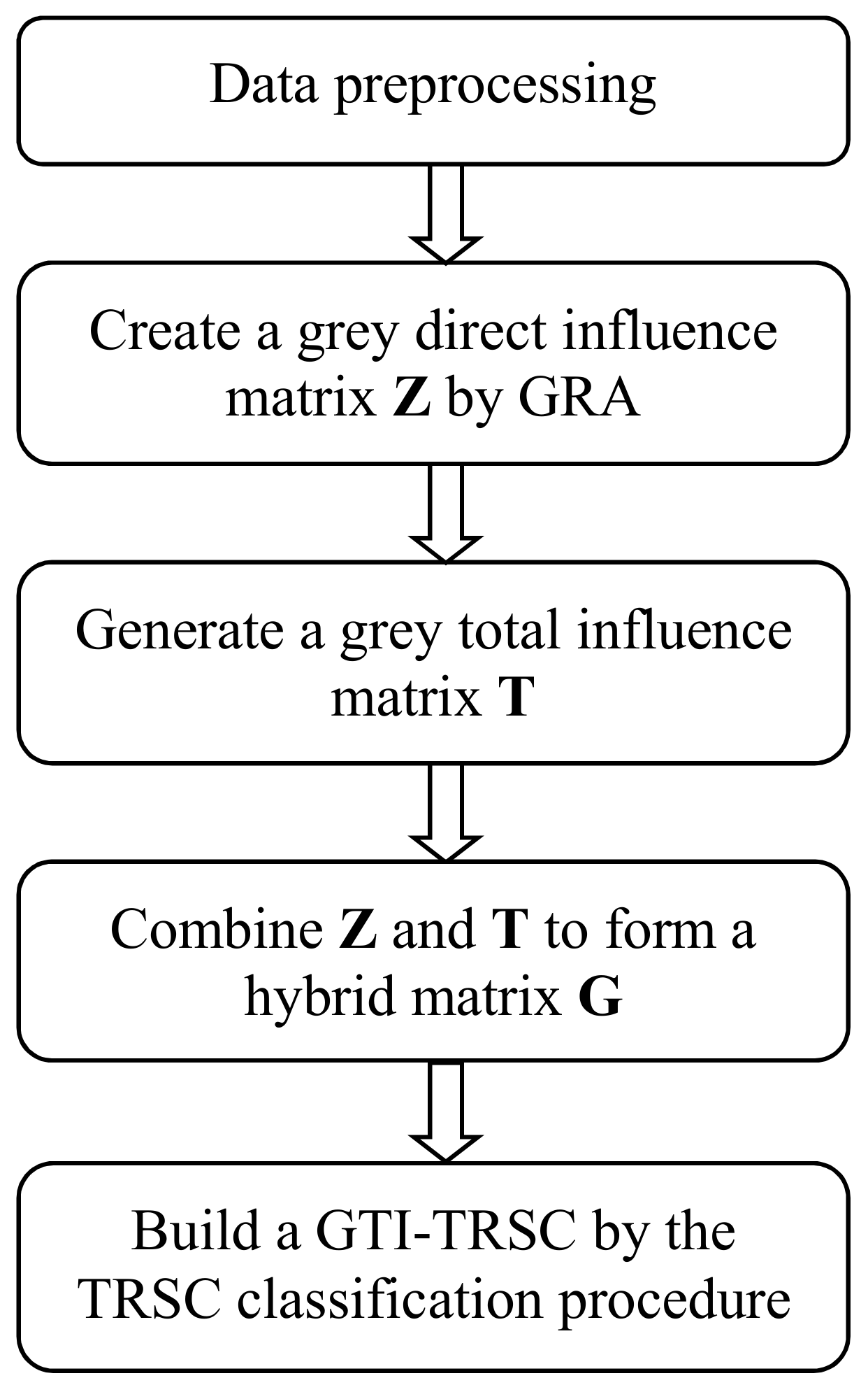
Evaluate chromosomes: Each chromosome corresponds to a GTI-TRSC that can be generated by the process shown in Figure 1. For each pattern, determine the lower and upper approximations for a GTI-based tolerance class. Furthermore, correct classification serves as a fitness function. Classification accuracy is the number of correct predictions made divided by the total number of predictions made, multiplied by 100 to turn it into a percentage.

(3)

Select: To produce generation k, randomly select two chromosomes from generation k − 1 by a binary tournament and place the one with higher fitness in a mating pool.

(4)

Crossover: Let $w_{i1}^k{w}_{i2}^k\dots w_{in}^k{\rho }_i^k{\alpha }_i^k{\tau }_i^k \mathrm{and} w_{j1}^k{w}_{j2}^k\dots w_{jn}^k{\rho }_j^k{\alpha }_j^k{\tau }_j^k$ be randomly selected chromosomes (1 ≤ i, j ≤ n_size) from generation k. Pr_c determines whether crossover can be performed on any two real-valued parameters. Two new chromosomes, $w_{i1}^{k-new}{w}_{i2}^{k-new}\dots w_{in}^{k-new}{\rho }_i^{k-new}{\alpha }_i^{k-new}{\tau }_i^{k-new} \mathrm{and} w_{j1}^{k-new}{w}_{j2}^{k-new}\dots w_{jn}^{k-new}{\rho }_j^{k-new}{\alpha }_j^{k-new}{\tau }_j^{k-new}$ are generated and are added into P_k+1. The related crossover operations are performed as:

$$\begin{array}{cc}{w}_{iw}^{k-new}\hfill & =a_w{w}_{iw}^k+\left(1-a_w\right)w_{jw}^k, w_{jw}^{k-new}= \left(1-a_w\right)w_{iw}^k+a_w{w}_{jw}^k\left(1 \le w\le n\right)\hfill \\ {\rho }_i^{k-new}\hfill & =b{\rho }_i^k+ \left(1-b\right){\rho }_j^k, {\rho }_i^{k-new}= \left(1-b\right){\rho }_i^k+b{\rho }_j^k\hfill \\ {\alpha }_i^{k-new}\hfill & =c{\alpha }_i^k+ \left(1-c\right){\alpha }_j^k, {\alpha }_i^{k-new}= \left(1-b\right){\alpha }_i^k+b{\alpha }_j^k\hfill \\ {\tau }_i^{k-new}\hfill & =d{\tau }_i^k+ \left(1-d\right){\tau }_j^k, {\tau }_j^{k-new}= \left(1-c\right){\tau }_i^k+c{\tau }_j^k\hfill \end{array}$$

where a_w, b, c, and d are random numbers ranging from zero to one.

(5)

Mutation: Pr_m determines whether a mutation can be performed on each real-valued parameter of a newly generated chromosome. With a mutation, the affected gene is altered by adding a random number selected from a prespecified interval, such as (−0.01, 0.01). A smaller Pr_m is required to avoid excessive perturbation.

(6)

Elitist strategy: Randomly remove n_del chromosomes from generation k. Insert n_del chromosomes with the maximum fitness from generation k − 1. A smaller n_del is required to generate a smaller perturbation in generation k.

(7)

Stopping rule: When n_max generations have been created, the algorithm reaches the stopping condition.

When the algorithm is terminated, the chromosome with the maximum fitness among all successive generations can be used to examine the generalization capability of the proposed GTI-TRSC.

5. Computer Simulations

As shown in

Table 2. Data used in computer simulations.

Data	# Patterns	# Attributes	# Classes
Australian approval	690	14	2
Glass	214	9	6
Hepatitis	155	19	2
Iris	150	4	3
Pima Indian diabetes	768	8	2
Sonar	208	60	2
Statlog Heart	270	13	2
Tic-Tac-Toe	958	9	2
Voting	435	16	2
Wine	178	13	3

, the generalization capability of the proposed GTI-TRSC was examined by experiments on some practical datasets available from the UCI Machine Learning Repository (http://www.ics.uci.edu/~mlearn/MLRepository.html). In Section 5.1, the performance of different rough-set-based classification methods is reported. Section 5.2 describes a statistical analysis to compare the different rough-set-based methods considered.

5.1. Evaluating Classification Performance

There is no optimal setting for parameter specifications for genetic algorithms, but we can refer to the principles introduced in [40,41]. Parameter specifications were specified for all experiments as follows: n_size = 50, n_max = 500, n_del = 2, Pr_c = 0.8, and Pr_m = 0.01. Five-fold cross-validation (5-CV) was considered for each classification method ten times by means of a distribution-balanced stratified CV (DBSCV) [42]. This study divided all patterns into five disjoint subsets of equal size such that four served as training patterns and one as test data. We iterated this procedure until each subset had been tested.

The classification performance of the proposed GTI-TRSC was compared with that of several representative rough-set-based classification methods: a rule-based method with shortening optimization (RSES-O) using the Rough Set Exploration System (RSES) [3,4,5], a hierarchical version of the lattice machine (HLM) [43,44], a hierarchical form of RSES-O (RSES-H) [44,45], and the Rule Induction with Optimal Neighborhood Algorithm (RIONA) [46]. These classification methods are briefly introduced as follows:

(1)

HLM: The lattice machine generates hypertuples as a model of the data. Some more general hypertuples can be used in the hierarchy that covers objects covered by the hypertuples. The covering hypertuples locate various levels of the hierarchy.

(2)

RSES-O: RSES-O is implemented in RSES. An optimal threshold for the positive region is used to shorten all decision rules with a minimal number of descriptors.

(3)

RSES-H: RSES-H can be obtained by constructing a hierarchy of rule-based classifiers. The levels of the hierarchy are defined by different levels of minimal rule shortening. A new pattern can be classified by a single hierarchy of the classifier.

(4)

RIONA: RIONA is also implemented in RSES. It uses the nearest neighbor method to induce distance-based rules. For a new pattern, the patterns most similar to it can vote for its decision, but patterns that do not match any rule are excluded from voting.

The classification performance of the above methods, reported in [44], is summarized in

Table 3. Classification accuracy of different classification methods. HLM: A hierarchical version of the lattice machine; RSES-O: a rule-based method with shortening optimization; RSES-H: A hierarchical form of RSES-O; RIONA: Rule Induction with Optimal Neighborhood Algorithm; TRSC: Tolerance-rough-set-based classifiers; SU: Subset approximations; CO: Concept approximations.

Dataset	Classification Methods
	HLM	RSES-H	RSES-O	RIONA	TRSC-SU	TRSC-CO
Australian approval	92.0	87.0	86.4	85.7	85.9	87.1
Glass	71.3	63.4	61.2	66.1	65.7	68.1
Hepatitis	78.7	81.9	82.6	82.0	83.9	83.5
Iris	94.1	95.5	94.9	94.4	95.7	95.2
Diabetes	72.6	73.8	73.8	75.4	74.1	73.6
Sonar	73.7	75.3	74.3	86.1	74.3	75.0
Statlog Heart	79.0	84.0	83.8	82.3	82.9	83.3
TTT	95.0	99.1	99.0	93.6	82.3	82.3
Voting	95.4	96.5	96.4	95.3	93.4	94.0
Wine	92.6	91.2	90.7	95.4	93.0	95.3
Average rank	9.20	7.90	8.80	8.80	9.55	9.15

.

Variants of TRSC were also considered: TRSC with subset approximations (TRSC-SU), TRSC with concept approximations (TRSC-CO), flow-based TRSC (FTRSC) with subset approximations (FTRSC-SU), flow-based TRSC with concept approximations (FTRSC-CO) [22], Grey-tolerance-rough- set-based classifier (GTRSC) with subset approximations (GTRSC-SU), and GTRSC with concept approximations (GTRSC-CO) [19]. The GTRSC and FTRSC were chosen because it is interesting to investigate whether different measures of similarity or relationship can influence classification accuracy. To implement the basic differences between GTI-TRSC, GTRSC, and FTRSC, GTRSC and FTRSC are briefly introduced as follows:

(1)

GTRSC: Instead of a simple distance measure used to evaluate the proximity of any two patterns, the GRG (grey relational grade) is used here to implement a relationship-based similarity measure that generates a tolerance class for each pattern. As mentioned above, only direct relationships were considered in the GTRSC.

(2)

FTRSC: The FTRSC uses preference information expressed by flows among patterns to measure similarity between patterns. The flow of each pattern is computed by the well-known preference ranking organization methods for enrichment evaluations (PROMETHEE) [47,48].

The results are summarized in Table 3 and

Table 4. Classification accuracy of TRSC variants. FTRSC: Flow-based TRSC; GTRSC: Grey-tolerance-rough- set-based classifier.

Dataset	Classification Methods
	FTRSC-SU	FTRSC-CO	GTRSC-SU	GTRSC-CO	GTI-TRSC-SU	GTI-TRSC-CO
Australian approval	88.0	87.7	89.3	89.1	91.0	90.9
Glass	69.1	69.4	70.1	69.9	79.8	79.7
Hepatitis	85.6	84.3	86.0	87.0	88.7	89.8
Iris	95.7	96.2	96.1	96.3	96.3	96.4
Diabetes	75.7	75.9	76.5	76.0	77.9	81.6
Sonar	78.8	79.5	83.0	82.8	86.7	87.8
Statlog Heart	83.9	84.1	84.4	84.0	86.9	86.1
TTT	97.3	97.8	98.5	98.5	98.9	98.5
Voting	96.6	96.3	96.0	96.2	97.4	97.7
Wine	93.2	95.1	97.4	97.9	97.9	98.1
Average rank	6.35	5.60	4.40	4.55	2.00	1.80

. It is clear that the classification performance of GTI-TRSC was comparable to that of FTRSC and GTRSC. This means that different measures can impose a certain impact on classification results.

5.2. Statistical Analysis

The nonparametric Friedman test [49] was used to statistically analyze the aforementioned classification methods. Using the null hypothesis, whereby the ranks of the classification methods were identical on average, the F_F statistic, distributed as an F distribution with k₁ − 1 and (k₁ − 1) (k₂ − 1) degrees of freedom, can be defined as follows [20]:

$$F_F=\frac{(k_2-1){\chi }_F^2}{k_2(k_1-1)-{\chi }_F^2}$$

(43)

where r_j, k₁, and k₂ are the average rank of method j, the number of methods, and the number of datasets considered, respectively. ${\chi }_F^2$ is defined as

$${\chi }_F^2=\frac{12k_2}{k_1(k_1+1)}[{\displaystyle \sum _{j=1}^{k_1}{r}_j^2}-\frac{k_1{(k_1+1)}^2}{4}]$$

(44)

F_F is 14.09 because k₁ = 12, k₂ = 10, and ${\chi }_F^2$ = 67.13. The null hypothesis was rejected at the 5% level as F_F was above the critical value of 1.98 (i.e., F(9, 99)).

Subsequently, the Nemenyi test [50] was used to detect significant differences among the classification methods. The classification accuracies of the two methods were significantly different and the differences in their average ranks were greater than CD:

$$CD=q_{\alpha }\sqrt{\frac{k_1(k_1+1)}{6k_2}}$$

(45)

where CD is a critical difference, and CD = 4.89 because q_0.10 = 3.03 at the 10% level. We summarize the results as follows:

(1)

GTI-TRSC-SU significantly outperformed TRSC-CO (9.15 − 2 = 7.15), TRSC-SU (9.55 − 2 = 7.55), RSES-H (7.90 − 2 = 5.90), RSES-O (8.80 − 2 = 6.00), RIONA (8.80 − 2 = 6.80), and HLM (9.20 − 2 = 7.2).

(2)

GTI-TRSC-CO significantly outperformed TRSC-CO (9.15 − 1.80 = 7.35), TRSC-SU (9.55 − 1.80 = 7.75), RSES-H (7.90 − 1.80 = 6.10), RSES-O (8.80 − 1.80 = 6.20), RIONA (8.80 − 1.80 = 7.00), and HLM (9.20 − 1.80 = 7.40).

(3)

There was no significant difference between GTI-TRSC and GTRSC for both set and concept approximations. Even so, GTI-TRSC outperformed GTRSC on seven out of ten datasets.

(4)

Although GTI-TRSC did not significantly outperform the FTRSC, the difference between GTI-TRSC-CO and FTRSC-SU was slightly less than CD (6.35 − 1.80 = 4.50). Therefore, it is reasonable to conclude that GTI-TRSC-CO was superior to FTRSC-SU. Even so, it is interesting to investigate the applications that can render GTI-TRSC and FTRSC significantly different.

6. Discussion and Conclusions

From the perspective of numerous or few relationships between any pair of patterns, this study used GRA to identify direct influences among patterns. A total influence matrix was generated to verify the direct/indirect influences among them. The total influence formed the foundation of the proposed GTI-TRS associated with the construction of the TRSC. The idea is that the higher the value of g_ij, the more similar x_i is to x_j. We noted that [19] had proposed grey tolerance rough sets (GTRS), which defined an overall similarity measure $S_A^G$(x_i, x_j), so that $S_A^G$(x_i, x_j) = ϒ(x_i, x_j). Therefore, the main difference between the GTRS and the GTI-TRS is that the former considers only direct relationships, but the latter considers direct as well as indirect relationships using the proposed grey total influence matrix. In particular, a GA was implemented to determine the optimal parameter specification for the proposed GTI-TRSC that cannot be easily determined by users.

Even though parameter specifications for GA are subjective, experimental results showed that the chosen parameters were acceptable. Indeed, the proposed GTI-TRSC is sufficiently simple to implement as a computer program without conforming to any statistical assumptions. Experimental results obtained by the proposed GTI-TRSC are promising. We see that GTI-TRSC-CO and GTI-TRSC-SU produced satisfactory results compared with the other rough-set-based classification methods considered. In particular, these two classifiers were superior in terms of classification performance to the TRSC. However, it should be noted that there is no best classifier [42].

This study has motivated us to investigate the subject further. As mentioned above, the grey DEMATEL has been an important issue for multiple attribute decision making. It is interesting to examine a distinctive version of the grey DEMATEL built on the proposed grey direct influence matrix. First, a novel DEMATEL-based Analytic Network Process (DANP) proposed in [20] was used to avoid agonizing pairwise comparisons for the ANP by replacing the total influence matrix produced by the DEMATEL by directly using the unweighted supermatrix of the ANP. The DANP has gained considerable research attention in recent years due to its convenience [21,22,23,24,25,26,27,28,29,30,31,32,33,34,35,36,37,38,39,40,41,42,43,44,45,46,47,48,49,50,51,52]. It is interesting to explore its applicability to practical problems by incorporating the new version of the grey DEMATEL into DANP.

Second, considering decision-making in a fuzzy environment, the linguistic interpretation of elements of the grey direct influence matrix is challenging. In practical applications, it may be desirable that a linguistic term be generated from numerical data [41]. Linguistic values such as “low influence”, “medium influence”, and “high influence” associated with fuzzy sets can be considered. Such a linguistic grey direct influence matrix can then be incorporated into the DEMATEL for further processing.

Finally, the traditional GRG is implemented using the weighted-average method, where dependency among the attributes is not considered. However, an assumption of additivity may not be realistic in practical applications [53]. Thus, it is more useful to employ a nonadditive grey total influence matrix with a nonadditive GRG [54], and check the resultant impact on the performance of GTI-TRSC. The aforementioned grey DANP, fuzzy-grey-DEMATEL, and nonadditive grey DEMATEL will be investigated in future studies.

References

1. Pawlak, Z. Rough sets. Int. J. Comput. Inf. Sci. 1982, 11, 341–356. [Google Scholar] [CrossRef]
2. Pawlak, Z. Rough Sets: Theoretical Aspects of Reasoning about Data; Kluwer: Dordrecht, The Netherlands, 1991. [Google Scholar]
3. Bazan, J.G.; Szczuka, M. RSES and RSESlib-A collection of tools for rough set computation. In Lecture Notes in Computer Science; Figueira, W., Yao, Y., Eds.; Springer: Berlin, Germany, 2001; pp. 106–113. [Google Scholar]
4. Bazan, J.G.; Szczuka, M. The rough set exploration system. In Lecture Notes in Computer Science; James, F.P., Andrzej, S., Eds.; Springer: Berlin, Germany, 2005; pp. 37–56. [Google Scholar]
5. Bazan, J.G.; Szczuka, M.; Wroblewski, J. A new version of rough set exploration system. In Lecture Notes in Computer Science; Alpigini, J.J., Peters, J.F., Skowron, A., Zhong, N., Eds.; Springer: Berlin, Germany, 2002; pp. 397–404. [Google Scholar]
6. Pawlak, Z.; Skowron, A. Rough sets and boolean reasoning. Inf. Sci. 2007, 177, 41–73. [Google Scholar] [CrossRef]
7. Pokowski, L. Rough Sets: Mathematical Foundations; Physica-Verlag: Heudelberg, Germany, 2002. [Google Scholar]
8. Walczak, B.; Massart, D.L. Rough set theory. Chemom. Intell. Lab. Syst. 1999, 47, 1–16. [Google Scholar] [CrossRef]
9. Zhang, X.; Dai, J.; Yu, Y. On the union and intersection operations of rough sets based on various approximation spaces. Inf. Sci. 2015, 292, 214–229. [Google Scholar] [CrossRef]
10. Shu, W.; Shen, H. Incremental feature selection based on rough set in dynamic incomplete data. Pattern Recognit. 2014, 47, 3890–3906. [Google Scholar] [CrossRef]
11. Jensen, R.; Shen, Q. Tolerance-based and fuzzy-rough feature selection. In Proceedings of the IEEE International Conference on Fuzzy Systems (FUZZ-IEEE’07), London, UK, 23–26 July 2007; pp. 877–882. [Google Scholar]
12. Parthaláin, N.M.; Shen, Q. Exploring the boundary region of tolerance rough sets for feature selection. Pattern Recognit. 2009, 42, 655–667. [Google Scholar] [CrossRef] [Green Version]
13. Stepaniuk, J. Rough Granular Computing in Knowledge Discovery and Data Mining; Springer: Berlin, Germany, 2008. [Google Scholar]
14. Kim, D.; Bang, S.Y. A handwritten numeral character classification using tolerant rough set. IEEE Trans. Pattern Anal. Mach. Intell. 2000, 22, 923–937. [Google Scholar]
15. Kim, D. Data classification based on tolerant rough set. Pattern Recognit. 2001, 34, 1613–1624. [Google Scholar] [CrossRef]
16. Ma, J.; Hasi, B. Remote sensing data classification using tolerant rough set and neural networks. Sci. China Ser. D Earth Sci. 2005, 48, 2251–2259. [Google Scholar] [CrossRef]
17. Skowron, A.; Stepaniuk, J. Tolerance approximation spaces. Fund. Inform. 1996, 27, 245–253. [Google Scholar]
18. Yun, O.; Ma, J. Land cover classification based on tolerant rough set. Int. J. Remote Sens. 2006, 27, 3041–3047. [Google Scholar] [CrossRef]
19. Hu, Y.C. Pattern classification using grey tolerance rough sets. Kybernetes 2016, 45, 266–281. [Google Scholar] [CrossRef]
20. Yang, Y.P.O.; Shieh, H.M.; Leu, J.D.; Tzeng, G.H. A novel hybrid MCDM model combined with DEMATEL and ANP with applications. Int. J. Oper. Res. 2008, 5, 160–168. [Google Scholar]
21. Peng, K.H.; Tzeng, G.H. A hybrid dynamic MADM model for problems-improvement in economics and business. Technol. Econ. Dev. Econ. 2013, 19, 638–660. [Google Scholar] [CrossRef]
22. Hu, Y.C. Flow-based tolerance rough sets for pattern classification. Appl. Soft Comput. 2015, 27, 322–331. [Google Scholar] [CrossRef]
23. Hu, Y.C. Tolerance rough sets for pattern classification using multiple grey single-layer perceptrons. Neurocomputing 2016, 179, 144–151. [Google Scholar] [CrossRef]
24. Tzeng, G.H.; Huang, J.J. Multiple Attribute Decision Making: Methods and Applications; CRC Press: Boca Raton, FL, USA, 2011. [Google Scholar]
25. Lin, C.L.; Hsieh, M.S.; Tzeng, G.H. Evaluating vehicle telematics system by using a novel MCDM techniques with dependence and feedback. Expert Syst. Appl. 2010, 37, 6723–6736. [Google Scholar] [CrossRef]
26. Grzymala-Busse, J.W.; Siddhaye, S. Rough set approaches to rule induction from incomplete data. In Proceedings of the International Conference on Information Processing and Management of Uncertainty in Knowledge-Based Systems, Perugia, Italy, 4–9 July 2004; pp. 923–930. [Google Scholar]
27. Liu, S.; Lin, Y. Grey Information: Theory and Practical Applications; Springer-Lerlag: London, UK, 2006. [Google Scholar]
28. Hu, Y.C.; Chen, R.S.; Hsu, Y.T.; Tzeng, G.H. Grey self-organizing feature maps. Neurocomputing 2002, 48, 863–877. [Google Scholar] [CrossRef]
29. Deng, J.L. Control problems of grey systems. Syst. Control Lett. 1982, 1, 288–294. [Google Scholar]
30. Bai, C.; Sarkis, J. A grey-based DEMATEL model for evaluating business process management critical success factors. Int. J. Prod. Econ. 2013, 146, 281–292. [Google Scholar] [CrossRef]
31. Liang, H.W.; Ren, J.Z.; Gao, Z.Q.; Gao, S.Z.; Luo, X.; Dong, L.; Scipioni, A. Identification of critical success factors for sustainable development of biofuel industry in China based on grey decision-making trial and evaluation laboratory (DEMATEL). J. Clean. Prod. 2016, 131, 500–508. [Google Scholar] [CrossRef]
32. Asad, M.M.; Mohajerani, N.S.; Nourseresh, M. Prioritizing Factors Affecting Customer Satisfaction in the Internet Banking System Based on Cause and Effect Relationships. Procedia Econ. Financ. 2016, 36, 210–219. [Google Scholar] [CrossRef]
33. Rajesh, R.; Ravi, V. Modeling enablers of supply chain risk mitigation in electronic supply chains: A Grey-DEMATEL approach. Comput. Ind. Eng. 2015, 87, 126–139. [Google Scholar] [CrossRef]
34. Shao, J.; Taisch, M.; Ortega-Mier, M. A grey-DEcision-MAking Trial and Evaluation Laboratory (DEMATEL) analysis on the barriers between environmentally friendly products and consumers: Practitioners’ viewpoints on the European automobile industry. J. Clean. Prod. 2016, 112, 3185–3194. [Google Scholar] [CrossRef]
35. Su, C.M.; Horng, D.J.; Tseng, M.L.; Chiu, A.S.F.; Wu, K.J.; Chen, H.P. Improving sustainable supply chain management using a novel hierarchical grey-DEMATEL approach. J. Clean. Prod. 2016, 134, 469–481. [Google Scholar] [CrossRef]
36. Xia, X.Q.; Govindan, K.; Zhu, Q.H. Analyzing internal barriers for automotive parts remanufacturers in China using grey-DEMATEL approach. J. Clean. Prod. 2015, 87, 811–825. [Google Scholar] [CrossRef]
37. Goldberg, D.E. Genetic Algorithms in Search, Optimization, and Machine Learning; Addison-Wesley: Boston, MA, USA, 1989. [Google Scholar]
38. Man, K.F.; Tang, K.S.; Kwong, S. Genetic Algorithms: Concepts and Designs; Springer: London, UK, 1999. [Google Scholar]
39. Rooij, A.J.F.; Jain, L.C.; Johnson, R.P. Neural Network Training Using Genetic Algorithms; World Scientific: Singapore, 1996. [Google Scholar]
40. Osyczka, A. Evolutionary Algorithms for Single and Multicriteria Design Optimization; Physica-Verlag: New York, NY, USA, 2002. [Google Scholar]
41. Ishibuchi, H.; Nakashima, T.; Nii, M. Classification and Modeling with Linguistic Information Granules: Advanced Approaches to Linguistic Data Mining; Springer: Heidelberg, Germany, 2004. [Google Scholar]
42. Zeng, X.; Martinez, T.R. Distribution-balanced stratified cross-validation for accuracy estimation. J. Exp. Theor. Artif. Intell. 2000, 12, 1–12. [Google Scholar] [CrossRef]
43. Wang, H.; Düntsch, I.; Gediga, G.; Skowron, A. Hyperrelations in version space. Int. J. Approx. Reason. 2004, 36, 223–241. [Google Scholar] [CrossRef]
44. Skowron, A.; Wang, H.; Wojna, A.; Bazan, J.G. Multimodal classification: Case studies. In Lecture Notes in Computer Science 4100; Peters, J.F., Skowron, A., Eds.; Springer: Berlin, Germany, 2006; pp. 224–239. [Google Scholar]
45. Skowron, A.; Wang, H.; Wojna, A.; Bazan, J. A hierarchical approach to multimodal classification. In Lecture Notes in Artificial Intelligence 3642; Slezak, D., Yao, J.T., Peters, J.F., Ziarko, W., Hu, X., Eds.; Springer: Berlin, Germany, 2005; pp. 119–127. [Google Scholar]
46. Bazan, J.G.; Szczuka, M.; Wojna, A.; Wojnarski, M. On the evolution of rough set exploration system. In Lecture Notes in Artificial Intelligence 3066; Tsumoto, S., Słowiński, R., Komorowski, J., Grzymala-Busse, J.W., Eds.; Springer: Heidelberg, Germany, 2004; pp. 592–601. [Google Scholar]
47. Brans, J.P.; Marechal, B.; Vincke, P. PROMETHEE: A new family of outranking methods in multicriteria analysis. Oper. Res. 1984, 84, 477–490. [Google Scholar]
48. Brans, J.P.; Vincke, P.; Marechal, B. How to select and how to rank projects: The PROMETHEE method. Eur. J. Oper. Res. 1986, 24, 228–238. [Google Scholar] [CrossRef]
49. Friedman, M. A comparison of alternative tests of significance for the problem of m rankings. Ann. Math. Stat. 1940, 11, 86–92. [Google Scholar] [CrossRef]
50. Nemenyi, P.B. Distribution-Free Multiple Comparisons. Ph.D. Thesis, Princeton University, Princeton, NJ, USA, 1963. [Google Scholar]
51. Hu, Y.C.; Chiu, Y.J.; Hsu, C.S.; Chang, Y.Y. Identifying key factors of introducing GPS-based fleet management systems to the logistics industry. Math. Probl. Eng. 2015. [Google Scholar] [CrossRef]
52. Hu, J.W.S.; Hu, Y.C.; Yang, T.P. DEMATEL and analytic network process for evaluating stock trade strategies using Livermore’s key price logic. Univers. J. Account. Finance 2017, 5, 18–35. [Google Scholar]
53. Wang, W.; Wang, Z.; Klir, G.J. Genetic algorithms for determining fuzzy measures from data. J. Intell. Fuzzy Syst. 1998, 6, 171–183. [Google Scholar]
54. Hu, Y.C. Nonadditive grey single-layer perceptron with Choquet integral for pattern classification problems using genetic algorithms. Neurocomputing 2008, 72, 332–341. [Google Scholar] [CrossRef]
Figure 1. A flowchart for constructing the proposed classifier (GRA: Grey Relational Analysis, GTI-TRS: grey-total-influence-based tolerance rough set).
Applsci 08 01173 g001