An Integrated Self-Diagnosis System for an Autonomous Vehicle Based on an IoT Gateway and Deep Learning

Abstract

This paper proposes “An Integrated Self-diagnosis System (ISS) for an Autonomous Vehicle based on an Internet of Things (IoT) Gateway and Deep Learning” that collects information from the sensors of an autonomous vehicle, diagnoses itself, and the influence between its parts by using Deep Learning and informs the driver of the result. The ISS consists of three modules. The first In-Vehicle Gateway Module (In-VGM) collects the data from the in-vehicle sensors, consisting of media data like a black box, driving radar, and the control messages of the vehicle, and transfers each of the data collected through each Controller Area Network (CAN), FlexRay, and Media Oriented Systems Transport (MOST) protocols to the on-board diagnostics (OBD) or the actuators. The data collected from the in-vehicle sensors is transferred to the CAN or FlexRay protocol and the media data collected while driving is transferred to the MOST protocol. Various types of messages transferred are transformed into a destination protocol message type. The second Optimized Deep Learning Module (ODLM) creates the Training Dataset on the basis of the data collected from the in-vehicle sensors and reasons the risk of the vehicle parts and consumables and the risk of the other parts influenced by a defective part. It diagnoses the vehicle’s total condition risk. The third Data Processing Module (DPM) is based on Edge Computing and has an Edge Computing based Self-diagnosis Service (ECSS) to improve the self-diagnosis speed and reduce the system overhead, while a V2X based Accident Notification Service (VANS) informs the adjacent vehicles and infrastructures of the self-diagnosis result analyzed by the OBD. This paper improves upon the simultaneous message transmission efficiency through the In-VGM by 15.25% and diminishes the learning error rate of a Neural Network algorithm through the ODLM by about 5.5%. Therefore, in addition, by transferring the self-diagnosis information and by managing the time to replace the car parts of an autonomous driving vehicle safely, this reduces loss of life and overall cost.

1. Introduction

The self-driving, autonomous vehicle has been getting lots of attention, due to significant developmental efforts and dramatic progress made by companies such as Google. While general use of autonomous vehicles for widespread use on public roads is likely years away, these vehicles are already being employed in “constrained” applications, such as open-pit mines and farming. Among the many technologies that make autonomous vehicles possible is a combination of sensors and actuators, sophisticated algorithms, and powerful processors to execute software [1]. With Tesla’s recent announcement of a semi-autonomous vehicle and Google’s strides in testing self-driving cars, we are beginning to see the first signs of a driverless future [2].

A vehicle with autonomous driving capability may be configured to receive signal inputs from the sensors that monitor the vehicle’s operations, surrounding objects, and road conditions in order to identify safety hazards and generate countermeasures to deal with various driving situations. The autonomous vehicle may also collect and record data from various information sources such as the cellular network, satellites, as well as user inputs such as a user’s identification, destinations and routes of navigation requests, and vehicle operation preferences. A vehicle with autonomous driving capability may further be adapted to detect various potential hazardous conditions and issue warnings to the user. The potential hazardous condition may include, for example, the vehicle's approaching a sharp curve, nearby pedestrians, or icy roads, etc. Such vehicle may also be configured with mechanisms that take active steps to avoid these hazards; e.g., slowing down the vehicle or applying the brake, etc. [3].

Cars have been diagnosing their own problems for decades, and to an extent, fixing themselves. Diagnosing and repairing faults is easy—dependent on the fault—but as software begins to drive the industry, surely it must be a question of big data?

Without a doubt, the cars of the future will be able to diagnose more faults and conditions than ever before. That particular feature of car ownership may be dramatically influenced by the Internet of Things, and software controlled hardware could possibly outlive any useful life. That doesn’t make vehicles self-repairing in the truest sense of the common meaning, but it does mean a huge step towards this goal.

This paper proposes “An Integrated Self-diagnosis System (ISS) for an Autonomous Vehicle based on an IoT Gateway and Deep Learning” which collects information from the sensors of an autonomous vehicle, diagnoses itself and the influence between parts by using Deep Learning and informs drivers of the result. The ISS consists of 3 modules.

The first In-Vehicle Gateway Module(In-VGM) collects the data from the in-vehicle sensors, the media data like a black box and a radar in driving, and the control message of a vehicle and transfers each data collected through each controller area network (CAN), FlexRay and Media Oriented Systems Transport (MOST) protocol to on-board diagnostics (OBD) or actuators. The data collected from the in-vehicle sensors is transferred to the CAN or FlexRay protocol and the media data in driving is transferred to the MOST protocol. Various types of messages transferred like this are transformed into a destination protocol message type. The second Optimized Deep Learning Module (ODLM) creates the Training Dataset on the basis of the data collected from the in-vehicle sensors and reasons the risk of the vehicle parts and consumables and the risk of the other parts influenced by a defective part. It diagnoses the risk of a vehicle’s total condition. The third Data Processing Module (DPM), based on Edge Computing, has an Edge Computing based Self-diagnosis Service (ECSS) to improve the self-diagnosis speed and reduce the system overhead, while a V2X based Accident Notification Service (VANS) informs adjacent vehicles and infrastructures of the self-diagnosis result analyzed by the OBD.

2. Related Works

2.1. In-Vehicle Internet of Things (IoT) Gateway

The CAN communication, which is the standard for most vehicles today, cannot process a large number of sensor data in real time [4]. Therefore, recent research has deployed FlexRay [5], which is a high speed protocol, or MOST [6], which is a high speed optical communication network of multimedia devices, to solve the sensor data problem. Figure 1a shows how these protocols are used with the CAN protocol. Other research improves upon the CAN protocol. Figure 1b shows that the Gateway uses the improved CAN protocol.

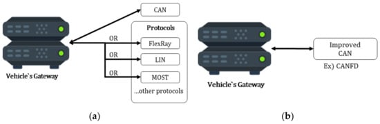
Figure 1. Controller Area Network (CAN) protocol. (a) CAN protocol; (b) Improved CAN protocol.

For example, a fast gateway [7] using FlexRay and CAN was proposed using FlexRay and CAN. A CAN controller and a FlexRay controller are designed with software (SW) and hardware (HW), respectively. The study did not consider the MOST protocol, but it reduced the run time by up to 94.7%.

A FlexRay-MOST gateway [8] using static segments and control messages was designed. The proposed gateway system is designed with Verilog hardware description language (HDL) and implemented using system-on-a-chip (SoC) kits. A reliable gateway [9] for communication between the local interconnect network (LIN), CAN, FlexRay protocols is presented. The main function of this gateway is translation.

It proposes a reliable gateway based on OSEK OS and OSEK NM for In-Vehicle Networks (IVNs). However, this gateway does not include the fault-tolerant mechanism. It will improve the reliability and safety of the gateway by adding the fault-tolerant mechanism that is called OSEK FTCOM.

A gateway framework for IVNs is proposed based on CAN, FlexRay, and Ethernet [10]. The gateway framework provides state-of-the-art functionalities that include parallel reprogramming, diagnostic routing, Network Management (NM), dynamic routing update, multiple routing configuration, and security. Ethernet can provide the required bandwidth, and it has several advantages for use in IVNs, including low cost, high bandwidth, and mature technology.

Combined with the idea of mobile cloud services, a new network architecture and data transmission method is proposed [11]. The proposed method can obtain a shorter transmission delay and ensure a higher transmission success rate. The timing impact introduced by various CAN/Ethernet multiplexing strategies at the gateways is determined [12]. They present a formal analysis method to derive upper bounds on end-to-end latencies for complex multiplexing strategies, which is the key for the design of safety-critical real-time systems.

A FlexRay-CAN gateway using a node-mapping method to overcome the message-mapping-based FlexRay-CAN gateway for a vehicle is presented [13]. A synchronization mechanism for FlexRay and Ethernet Audio Video Bridging (AVB) network that guarantees a high quality-of-service is proposed [14]. The synchronization mechanism provides timing guarantees for the FlexRay network that is similar to those of the Ethernet AVB network.

Ju proposes a novel gateway discovery algorithm for communication between VANETs and 3G, providing an efficient and adaptive Location-Aided and Prompt Gateway Discovery (LAPGD) mechanism [15]. Aljeri proposes a reliable QoS-aware and location aided gateway discovery protocol for vehicular networks by the name of fault tolerant location-based gateway advertisement and discovery. Their proposed protocol succeeded in balancing the load between gateways with the presence of gateway and road component failures [16].

A reliable gateway for in-vehicle networks is described. Such networks include local interconnect networks, controller area networks, and FlexRay. It is proposed a reliable gateway based on the OSEK/VDX components for in-vehicle networks [17].

The various actual arriving orders of gateway messages are examined in detail and then an explorative Worst-Case Response Time (WCRT) computation method is proposed. It is proved that the obtained WCRT results are safe WCRT bounds. The method proposed by this paper reduced WCRT by 24% [4]. A gateway system for a mix of CAN and controller area network flexible data-rate (CANFD) networks using a valid routing method is proposed. This method applies to several cases for validation purposes. When CANFD messages are routed, the memory buffer in the ring structure enables sequential routing without data loss [18].

Seo proposes a Universal Plug And Play (UPnP)-CAN gateway system using UPnP middleware for interoperability between external smart devices and an in-vehicle network. The proposed gateway consists of a UPnP communication device, a CAN communication device, and a device translator layer. The CAN communication device transmits and receives real-time vehicle data between the real vehicular simulator and external devices through the UPnP. The device translator layer configures a message frame for enabling seamless data input and output between the CAN and UPnP protocols [19].

This paper proposes a gateway that supports the MOST, FlexRay, and CAN protocols. To improve compatibility between protocols, different types of data are converted into the same message format. It supports reliable real-time communication and proposes an internal gateway scheduler to solve the data transmission delay problem.

2.2. Fault Diagnosis of a Vehicle

Currently, most self-diagnostics for vehicles use non-OEM or OEM-based OBD methods [20,21,22]. However, they do not use any neural network model. In case of a neural network used for a vehicle, studies are underway on electric vehicles and connected vehicles. Besides, there is active research in various fields. Some of these studies diagnose the failure of a particular system in a vehicle through a deep-learning method. So we briefly describe those studies. The following are examples about studies that use neural network in vehicles.

The sensor abrupt-faults of Hybrid Electric Vehicles (HEV) control system are focused. A novel method for diagnosing sensor abrupt-faults is proposed based on the Wavelet Packet Neural Network (WPNN). It puts the feature data that have been normalized as the input vector of the WPNN and trains the neural network. Then the features of a fault signal can be effectively identified [23].

A new data compression approach is provided and validated on a method based on Neural Network (NN) to detect both failure type and degree in a driving system. A brief method was introduced to preprocess training data by analyzing the linear relationship between features and patterns to be classified. This indicates that the proposed method used to preprocess data can significantly improve the efficiency and precision in categorizing all the fault samples, especially for the fault degrees considered in this study [24].

An Artificial Neural Network (ANN)-based fault diagnosis method after extraction of a new pattern is proposed. ANN is a neural network that sets various features of the converter as parameters. The new pattern of an AC-DC converter failure in view of SHEV application has been used as the training data of the ANN [25].

The diagnosis method based on a wavelet and neural network is proposed. This method does not need to collect a large number of data, but simplifies the diagnostic process while ensuring the accuracy of the diagnostic result. Chuang focuses on the Self-Organizing feature Map (SOM) neural network to diagnose the stator winding faults in the Permanent Magnet Synchronous Motor (PMSM). In order to train and work easily about the network, the fault feature data was extracted from the current sample by using the Wavelet Transform (see Figure 2). This method uses only stator currents as raw data; the energy of high frequency in the current is extracted based on the wavelet transform and then the energy is used as the fault feature after the normalizing processing [26].

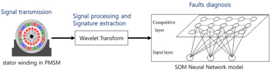
Figure 2. Process of diagnosis health and stator winding fault in Permanent Magnet Synchronous Motor (PMSM).

Yurii examines an approach to increasing the safety of a vehicle’s design with the help of ANNs integrated in the vehicle’s self-diagnostic system. The method that is proposed to improve the safety of the vehicle’s structural design based on artificial neural networks that are integrated in the self-diagnostic system, and these help to ensure a fast response due to the parallel processing of the flows of diagnostic information from the different nodes, assembly units, and systems, as well as increasing the credibility of the diagnostic state of the electronic systems. This also includes processing of individual information about the previous states of the systems of some specific vehicles. However, this suggestion is theoretical and there is no experimental data [27].

In order to avoid the interference and coupling of the control channels between Active Front Steering (AFS) and Active Suspension Subsystems (ASS), Chunyan presents a composite decoupling control method, which consists of a neural network inverse system and a robust controller. The neural network inverse system is composed of a static neural network with several integrators and state feedback of the original chassis system to approach the inverse system of the nonlinear systems [28].

Chu proposes a novel vehicle detection scheme based on multi-task deep Convolutional Neural Networks (CNNs) and Region-Of-Interest (RoI) voting. In the design of the CNN architecture, this study enriches the supervised information with subcategory, region overlap, bounding-box regression, and a category for each training RoI as a multi-task learning framework [29].

Liu proposes a method, which integrates deep neural networks with balanced sampling to address the challenges of classifying imbalanced data acquired from visual traffic surveillance sensors. The proposed method is able to enhance the mean precision of all the categories, in the condition of high overall accuracy [30].

A Lane Departure Prediction (LDP) method based on the Monte Carlo simulation and a Deep Fourier Neural Network (DFNN) is proposed to make improvements on the vision-based Lane Departure Warning Systems (LDWS). The proposed technique enhances the system’s functions of the over-speed warning on a curved road and the over-steer warning on a low-adhesion road [31].

A probabilistic model named the Collision Prediction model based on a GA-optimized Neural Network (CPGNN) for decision-making in the rear-end collision avoidance system is proposed [32].

Wang presents a novel method to detect vehicles using a far infrared automotive sensor. Firstly, vehicle candidates are generated using a constant threshold from the infrared frame. Contours are then generated by using a local adaptive threshold based on maximum distance, which decreases the number of processing regions for classification and reduces the false positive rate. Finally, vehicle candidates are verified using a Deep Belief Network (DBN) based classifier. This study is approximately a 2.5% improvement on previously reported methods and the false detection rate is also the lowest among them [33].

George uses the process of real-time intrusion detection on a robotic vehicle. This study shows that by offloading this task to a remote server, we can utilize approaches of much greater complexity and detection strength based on deep learning [34].

A novel framework is proposed for vehicle Make and Model Recognition (MMR) using local tiled deep networks. A Local Tiled Convolutional Neural Network (LTCNN) is proposed to alter the weight sharing scheme of a CNN with a local tiled structure. This architecture provides the translational, rotational, and scale invariance as well as the locality. The experimental results show that their LTCNN framework achieved a 98% accuracy rate in terms of vehicle MMR [35].

Liujuan investigates the possibility of exploiting deep neural features towards robust vehicle detection and a vehicle detection framework, which combines Deep Convolutional Neural Network (DCNN) based feature learning with an Exemplar-SVMs (E-SVMS) based, robust instance classifier to achieve robust vehicle detection in satellite images. Their models show that the combination of both schemes can benefit from each other to jointly improve the detection accuracy and effectiveness [36].

Meng firstly puts forward a new memetic evolutionary algorithm, named the Monkey King Evolutionary (MKE) Algorithm, for global optimization. It gives an application of this algorithm to solve the least gasoline consumption optimization (find the least gasoline consumption path) for vehicle navigation. They use this algorithm to find the least gasoline consumption path in vehicle navigation, and have conducted experiments that show the proposed algorithm outperforms A* algorithm and the Dijkstra algorithm as well [37].

Zhao proposes a CNN model of visual attention for image classification. Their systematic experiments on a surveillance-nature dataset that contains images captured by surveillance cameras in the front view demonstrate that the proposed model is more competitive than the large-scale CNN in vehicle classification tasks [38].

A vehicle fault detection and diagnosis combining Auto Associative Neural Networks (AANN) and several Adaptive Neuro-Fuzzy Inference Systems (ANFIS) is proposed. This system is a process history based method; only normal operating conditions data are needed for training the system. The approach could tackle the problem of false alarms, due to the correlation among variables [39].

RBF neural network consensus-based distributed control scheme is proposed for non-holonomic autonomous vehicles in a pre-defined formation along the specified reference trajectory [40]. Luo proposed a deep convolution neural network that is no less than nine layers. Compared with a traditional vehicle recognition based on machine learning, which requires vehicle location and has low accuracy of shortcomings, the proposed model using a deep convolution neural network displays better performance [41].

Glowacz described an acoustic based fault diagnosis technique of the three-phase induction motor. Four states of the three-phase induction motor were analyzed: healthy three-phase induction motor, three-phase induction motor with broken rotor bar, three-phase induction motor with two broken rotor bars, and a three-phase induction motor with the faulty ring of a squirrel-cage. The proposed feature extraction methods: SMOFS-32-MULTIEXPANDED-2-GROUPS and SMOFS-32-MULTIEXPANDED-1-GROUP were analyzed. The Nearest Neighbor classifier, backpropagation neural network, and the modified classifier based on words coding were used for recognition. It can prevent unexpected failure and improve the maintenance of electric motors. Advantages of the acoustic based fault diagnosis technique are: non-invasive technique, low cost, and instant measurement of the acoustic signals [42].

Praveenkumar reports on the feasibility of performing vibrational monitoring in real world conditions; i.e., by running the vehicle on the road and performing the analysis. The data were acquired for the various conditions of the gearbox and features were extracted from the time-domain data and a decision tree was trained for the time-domain analysis. Fast Fourier Transform was performed to obtain the frequency domain, which was divided into segments of equal size and the area covered by the data in each segment was calculated for every segment to train the decision trees. The classification efficiencies of the decision trees were obtained and in an attempt to improve the classification of efficiencies, the time-domain, and a frequency-domain analysis was also performed on the normalized time-domain data [43].

Ganovska focuses on the problem of the prediction of surface roughness in AWJ process and contributes to the online monitoring of the hydro-abrasive material disintegration process and its possible control. The main scope of study is to contribute to the usage of an artificial neural network as a decisive part in surface roughness prediction and to outline a suitable online control mechanism [44].

Hu considers the usage of artificial intelligence, in particular, neural networks, to correct and compensate for thermocouple errors. Proposed in this paper are the correction of the thermocouple tolerance, the error due to the conversion characteristic drift under the influence of high operating temperatures as well as the compensation of the error due to acquired thermoelectric inhomogeneity of thermocouple legs. The corrections are carried out using individual mathematical models based on neural networks. The neural network method for controlling a temperature field to compensate for the error due to the acquired thermoelectric in-homogeneity is proposed [45].

In this paper, input nodes and output nodes are generated flexibly by receiving signals from all sensors. The input node is the number of sensors, and the output node is the number of parts to be diagnosed. That is, all the parts that can be measured by the sensors can be diagnosed. The generated neural network model is simulated using a Deep Belief Network (DBN) [46], Long Short Term Memory (LSTM) [47], and the proposed ODLM, which are learning models used in real-time processing.

3. An Integrated Self-Diagnosis System for an Autonomous Vehicle Based on an IoT Gateway and Deep Learning

3.1. Overview

Because an autonomous vehicle is one that can drive itself from a starting point to a predetermined destination in “autopilot” mode using various in-vehicle technologies and sensors, including adaptive cruise control, active steering (steer by wire), anti-lock braking system (brake by wire), GPS navigation technology, lasers and radar, it is important to accurately inform drivers of a failure and the failure causes about a vehicle while driving. If the failure and the failure causes are not transferred or are delayed, it brings about fatal consequences. To tackle these problems, this paper proposes “An Integrated Self-diagnosis System (ISS) for an Autonomous Vehicle based on an IoT Gateway and Deep Learning”, which collects information from the sensors of an autonomous vehicle, diagnoses itself by using Deep Learning, and informs the driver of the result.

The ISS consists of three modules as shown in Figure 3. The first In-VGM collects the data from the in-vehicle sensors, the media data like a black box and a radar in driving, and the control message of a vehicle, and transfers the data collected through each CAN, FlexRay, and MOST protocol to the OBD or actuators. The data collected from the in-vehicle sensors is transferred to the CAN or FlexRay protocol and the media data in driving is transferred to the MOST protocol. Various types of messages transferred like this are transformed into a message type of a destination protocol. The second ODLM creates the Training Dataset on the basis of the data collected from in-vehicle sensors and reasons the risk of the vehicle parts and consumables and the risk of the other parts influenced by a defective part. It diagnoses the risk of the vehicle’s total condition. The third DPM based on Edge Computing has the SS to improve the self-diagnosis speed and reduce the system overhead and the VANS to inform adjacent vehicles and infrastructures of the self-diagnosis result, which is analyzed by the OBD.

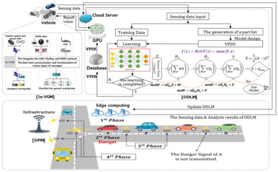
Figure 3. The Structure of an Integrated Self-diagnosis System (ISS).

3.2. A Design of an In-Vehicle Gateway Module (In-VGM)

The data types collected from the in-vehicle sensors are diverse. The existing CAN protocol has limits on transmission capacity and speed. However, even if the FlexRay and MOST protocol ensuring high communication speed, the exact transmission time is used instead of the CAN, as they might also have another problems such as cost and compatibility.

Therefore, this paper proposes the dedicated In-VGM which integrates the CAN, FlexRay, and MOST protocol to solve compatibility and distributed data transmission and ensures reliable and real time communication by transforming various types of messages into a message type of a destination protocol.

The existing in-vehicle gateway protocols like CAN, FlexRay, and MOST have the following problems.

• First, they do not use a multi-directional network.
• Second, they are inefficient and lack the overhead to transform messages in various protocols.
• Third, they have a transmission delay because they have no priority protocol in place to hierarchize individual messages in transferring multiple messages.
• Fourth, they do not ensure compatibility because an autonomous vehicle collects unstructured data like image, radar, and video.

However, the In-VGM proposed in this paper has the following functions to solve the above problems.

• First, it allocates ID to a CAN bus interface which collects and transfers the general sensing data of vehicles and to a FlexRay-CAN bus interface that collects and transfers the emergent sensing data of vehicles and to the MOST bus interface, which collects and transfers media data. It has a bus architecture connecting the interfaces.
• Second, it supports a multi-directional network because the mapping table with message transformation information is used for it.
• Third, it provides a priority based transmission mode to increases the transmission efficiency of messages based on an event and to reduce the transmission delay of important messages.
• Fourth, it uses an inner scheduler to reduce the transmission delay.

The In-VGM works as follows.

• First, the in-vehicle data is classified into general sensing data, emergent sensing data, control system and sensor data, media data, and OBD data. The CAN, FlexRay, and MOST protocols are used according to the importance and classification of data. The Bus architecture of the In-VGM is shown in Figure 4.
  

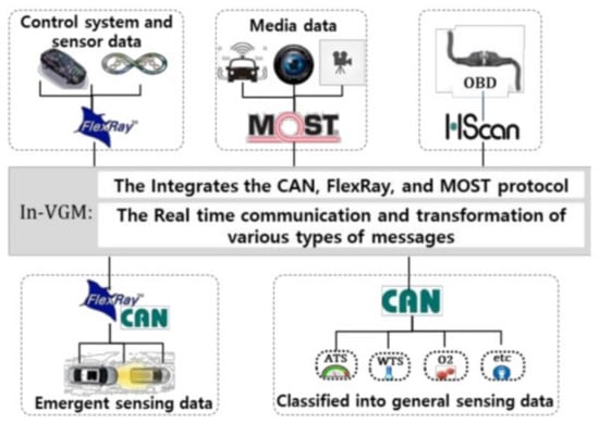  Figure 4. The structure of the In-Vehicle Gateway Module (In-VGM).
• Second, the data collected and transferred in the sensor and control system is transferred to the In-VGM through the CAN, FlexRay, and MOST protocols. At this time, the In-VGM allocates ID according to a sending and receiving CAN, FlexRay, and MOST protocol. The kinds of IDs are shown in Table 1.
  Table 1. The kinds of message IDs about protocols.

  No.	Source	Destination	ID
  1	CAN	CAN	10
  2		FlexRay	801
  3		MOST	811
  4		HSCAN	30
  5		FlexRayCAN	60
  6	FlexRay	CAN	803
  7		FlexRay	802
  8		MOST	812
  9		HSCAN	813
  10		FlexRayCAN	814
  ...	...	...	...
  24	MOST	HSCAN	821
  25		FlexRayCAN	823

• Third, the source and destination protocol ID of the transmission data are recorded in a mapping table and transmission paths are set on the basis of the ID. If the transmission paths are set, the transmission message type is transformed into a message type of a destination protocol by using the mapping table.
• Fourth, because the size of data collected and transferred by the FlexRay and MOST is very big, compared to that of the CAN, the header information like Start Message Delimiter, Length of message, and Identifier is to be added to every CAN Fragment so that the FlexRay and MOST data can be transferred to the CAN protocol. The Header information has a maximum of 35 bits.

In a multi-directional network environment, because the number of the headers gets larger in proportion to the number of the CAN fragments, the CAN has overhead. If the CAN message type is transformed into a message type of the FlexRay or the MOST protocol, the problem is that all the messages are not transferred because of the overhead of the headers. To solve the problem, the ID of the proposed CAN Fragment Header, instead of the Priority and Service type of the existing CAN fragment Header, is proposed and the Sequential Number of the proposed CAN Fragment Header instead of the Request, Destination ID, Service, and Source ID of the existing CAN Fragment Header is proposed. Because the In-VGM uses the Sequential Number of the CAN Fragment Header, it sorts the CAN fragments in the Mapping Table in ascending order and then transfers them to a destination where the CAN fragments are sorted in ascending order.

If the data is transformed and transferred after the Sequential Numbers are sorted, the In-VGM identifies the fragments of the CAN with Sequential Numbers and IDs. For example, in Figure 5, if the number of the CAN fragments is 20 and each fragment size is 4 bytes, the first fragment’s Sequential Number is 01, the next fragment is 02, 03, and 04 in order.

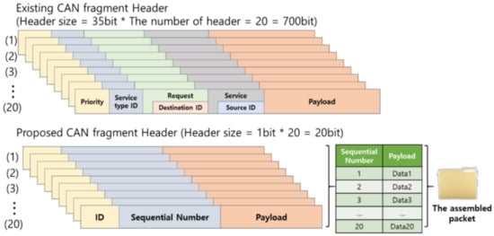
Figure 5. CAN fragment Header and fragment assembly process in the In-VGM.

When the CAN fragments are transferred to the FlexRay, the In-VGM assembles the fragments sequentially according to the Sequential Number and transfers the assembled packet.

3.3. A Design of an Optimized Deep Learning Module (ODLM)

The ODLM proposed in this paper works in a Cloud Environment and consists of two sub-modules.

The first Vehicle Part Diagnosis Sub-module (VPDS) diagnoses the condition of parts and of the other parts influenced by a defective part by using the data collected by the in-vehicle sensors. The second Total Diagnosis Sub-module (TDS) diagnoses the total condition by using the real-time sensor data of a vehicle and the result diagnosed by the VPDS as input data.

The ODLM generates a Training Data Set with the sensor data of a vehicle, starts a learning process and diagnoses the vehicle itself if the learning is completed. Through the cloud, the ODLM transfers to a vehicle the results of two submodules and the difference between the current sensor data and normal sensor data. The flowchart of the ODLM is shown in Figure 6.

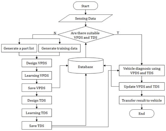
Figure 6. Flowchart about Optimized Deep Learning Module (ODLM).

3.3.1. A Design of the VPDS

The VPDS diagnoses the condition of the parts and of the other parts influenced by a defective part. To do this, the input and output value of the VPDS, the Hidden Layers of the VPDS and the VPDS Mathematical modeling must be decided as follows.

The Input and Output Value of the VPDS

The VPDS uses the sensor data received from the vehicle as the input value of the VPDS. The data collected from the in-vehicle sensors are digital numerical data and represents the condition of each part. The VPDS input is represented as $\mathrm{X}=\left\{x_1, x_2, x_3, x_4, \dots , x_n\right\}$. Here, X means the set of sensors, $x_n$ means the sensor data from each sensor, and n means the number of sensors. For example, a tire temperature sensor and a tire air pressure sensor measure the condition of a tire and an oil pressure sensor measures the condition of engine oil. The output value of the VPDS represents the condition of each part. Each part has three output nodes to diagnose its condition. The VPDS output is represented as $\mathrm{Y}=\left\{y_1, y_2, y_3, y_4, \dots , y_k\right\}$. Here, Y means the set of all output nodes, $y_k$ means the output value of each node, and the number of output nodes, k is 3 times the number of parts. Each node of each part represents “normal”, “check”, and “danger”.

Let us take 8 outputs of a tire for example. (1) If the normal node for the tire is 1 and the check node and the danger node are 0, then this means the tire is in a normal state. (2) If the check node for the tire is 1 and the normal node and the danger node are 0, then this means the tire is in a checking state. (3) If the danger node for the tire is 1 and the normal node and the check node are 0, then this means the tire is in a dangerous state. (4) If the normal node and the check node for the tire are 1 and the danger node are 0, then this means the tire is in a checking state. (5) If the danger node and the check node for the tire are 1 and the normal node are 0, then this means the tire is in a dangerous state. (6) If the normal node and the danger node for the tire are 1 and the check node are 0, then this means the condition of the tire cannot be judged. (7) If all three nodes of a tire are 0 or 1, then this means the condition of the tire cannot be judged. Figure 7 shows the 8 outputs of a tire.

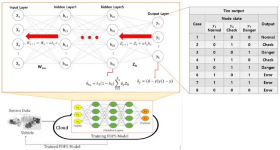
Figure 7. The structure of the Vehicle Part Diagnosis Sub-module (VPDS).

The Hidden Layers of the VPDS

Though an existing Back-propagation algorithm does not decide the number of Hidden Layers and the number of its Nodes, the proposed Back-propagation algorithm that is used by The VPDS decides the number of them dynamically according to the input sensor data and the number and types of output parts. If there are a number of input and output nodes and a number of Hidden Layers and their nodes, an over-fitting problem can occur. The VPDS in this paper limits the number of Hidden Layers to five to reduce the over-fitting. The number of Nodes in each Hidden Layer is equal to that of input nodes. The Nodes in each Hidden Layer are used to compute the risk of vehicle parts and consumables and the risk of the other parts influenced by a defective part.

The VPDS Mathematical Modeling

The VPDS uses a Back Propagation algorithm with high accuracy and speed for the safety of a vehicle. The Training Data made out of the sensor data are used for the learning of the VPDS. The Training Data are collected from the real time sensor data of a vehicle or the batch sensor data of a Car Service Center. The collected data are integrated numeric data about the normality and abnormality of each part. The Training Dataset is made out of the Training Data based on parts.

Figure 7 shows the structure of the VPDS. The h of the Hidden Layer means a node value. The vector of a Hidden Layer is $\mathrm{H}$. The $y$ of the Output Layer means the condition of the parts. The condition of the parts is classified into ‘danger’, ‘inspection’, and ‘normality’ by the result value of the Output Layer. W~Z represent the weight connecting to each Output Layer and are modified during learning. Formula (1) is the loss function of the VPDS.

$$\frac{1}{2}{\left(d-y\right)}^2$$

(1)

The VPDS uses the ReLU function and the Sigmoid function as an activation function, solves the vanishing gradient problem from an input layer to the last hidden layer by using an ReLU function, and diagnoses the result between the last hidden layer and an output layer by using a Sigmoid function.

The VPDS is processed in the following phases.

• The 1st phase: the weight W~Z are initialized as a small value, not 0 and Training Datasets are used.
• The 2nd phase: The initial learning rate and a critical value of an error, Emax are decided.
• The 3rd phase: The nodes’ values of the 1st Hidden Layer and the weight sum of the $h_{1j}$ of the 1st Hidden Layer by using Formula (2), $NE{T}_{h_{1j}}$ are obtained in the VPDS. At this time, the $x_i$ of Formula (2) means the value of the ith input node, and $W_{ij}$ means a weight between the ith input node and the jth Hidden Layer. The VPDS computes the $h_{1j}$, which is the node value of the 1st Hidden Layer by applying the $NE{T}_{h_{1j}}$ of the expression (3).

  $$NE{T}_{h_{1j}}={\displaystyle \sum }_{i=1}^n{x}_i{W}_{ij}$$

  (2)

  $$h_{1j}=\max \left(0, NE{T}_{h_{1j}}\right)$$

  (3)

In this way, the VPDS computes $NET$ and the Output value from the 1st hidden layer to the rest of the hidden layer.

• The 4th Phase: The VPDS computes the $NE{T}_{y_k}$ between the 5th hidden layer and an Output layer by using Formula (4) and computes the output value, $y_k$ by using Formula (5). The $NE{T}_{y_k}$ is applied to the Sigmoid function of Formula (5).

  $$NE{T}_{y_k}={\displaystyle \sum }_{i=1}^l{h}_{5i}{Z}_{ik}$$

  (4)

  $$y_k=\frac{1}{1+e^{-NE{T}_{y_k}}}$$

  (5)
• The 5th Phase: The VPDS computes an error E in the Formula (6) and compares it with the Emax of the 2nd Phase. The VPDS closes the learning if the error E is less than the Emax. The VPDS goes to the 5th Phase if the error E is greater than the Emax.

  $$\mathrm{E} =\frac{1}{2}{\displaystyle \sum }_{i=1}^k{\left(d_i-y_i\right)}^2$$

  (6)
  Here, $d_i$ means a target value and, $y_i$ is the result value of the Output Layer computed in the 3rd phase.
• The 6th Phase: The VPDS computes an error signal, ${\delta }_h$ between the Output Layer and the last Hidden Layer and between the Hidden Layers.

The process works as follows.

First, the VPDS computes the error signal, ${\delta }_y$ between the Output Layer and the last Hidden Layer by using the Formula (7).

$${\delta }_y=\left(d-y\right)y\left(1-y\right)$$

(7)

Second, It computes the error signal, ${\delta }_h$ between the Hidden Layers by using the Formula (8).

$${\delta }_{h_5}=h_5\left(1-h_5\right){\displaystyle \sum }_{i=1}^k{\delta }_y{Z}_{li}$$

(8)

Here, $h_5$ means the 5th Hidden Layer, ${\delta }_y$ means the error signal between Output Layer and the last Hidden Layer and $Z_{li}$ means the weight between the Output Layer and the last Hidden Layer. The VPDS computes the ${\delta }_{h_4}$~${\delta }_x$ in the same way as Formula (8).

• The 7th Phase: The VPDS modifies the weight, Z between the last Hidden Layer and Output Layer by using the Formula (9).

  $$Z_{k+1}=Z_k+\alpha {\delta }_y{h}_5.$$

  (9)
  Here, $Z_k$ means the weight before being modified and $Z_{k+1}$ means the weight after being modified. $\alpha$ means a learning rate, ${\delta }_y$ means the error signal computed by the Formula (8), and $h_5$ means the 5th Hidden Layer.

The VPDS modifies the weight from the 5th Hidden Layer to an input layer in the same way as Formula (8). For example, If the weight between the 1st Hidden Layer and an Input Layer is W, the W is modified in Formula (9).

$$W_{k+1}=W_k+\alpha {\delta }_{h_1}x$$

(10)

Here, $W_k$ means the weight before being modified and $W_{k+1}$ means the weight after being modified. And $\alpha$ means a learning rate, ${\delta }_{h_1}$ means the error signal of 1st Hidden Layer. And $x$ means nodes value of the Input Layer.

• The 8th Phase: the VPDS repeats the learning process (training) from the 3rd phase to the 7th phase till an error E becomes less than the Emax.

3.3.2. A Design of TDS

The TDS is a Lightweight Neural Network Module that diagnoses a vehicle’s total condition by entering each diagnosed result of the autonomous vehicle parts computed by the VPDS. The TDS of Figure 8 shows the Multiple Output Perceptron that sets the weights of the input nodes differently. That is, it shows a Lightweight Neural Network with a Step Function that has a critical value 0 as an Activation Function. For example, Figure 8 shows that the TDS judges total condition by integrating each analysis result of an engine, a tire, a headlight, and a generator etc. If the analysis result of the TDS is (1, 1, 0), it judges the total diagnosis result as “Check”.

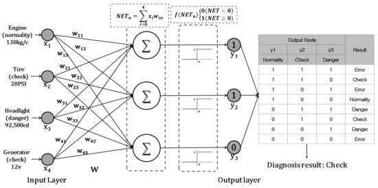
Figure 8. The example of the Total Diagnosis Sub-module (TDS) perceptron operation.

A Learning Method of the TDS

The TDS should set the learning method. The following Algorithm 1 is the Learning Algorithm of the TDS and works as follows.

Algorithm 1. TDS learning algorithm

TDS_Learning(VPDS Output, W[[], learning rate, Training Data Set){  k < −1  while(true) {   new-W <- W   for 1 to the number of the Training Data Sets{    NET <- VPDS Output * new-W    TDS-Output <- Step Function(NET)    if (TDS-Output == Training Data.out) {    }    else {     new-W <- learning rate * VPDS Output *         (Training Data.out–Output)    }   }   if (W == new-W) then End   else {    k < −k + 1    7W <- new-W   }  } }

• First, the TDS uses the VPDS output, the initial value of weight W[], the learning rate and the Training Data.
• Second, if the learning gets started, an existing weight W is assigned to the new-W.
• Third, the fourth and fifth phases are repeated as large as the number of the Training Data Sets is.
• Fourth the VPDS Output value multiplied by new-W is stored in the NET. Then, the result of a Step Function for NET is stored in the TDS-Output
• Fifth, if the TDS-Output is the same as the output of the learning data, the weight is not modified. If the TDS-Output is different from the output of the learning data, TDS modifies weight and stores it in the new-W.
• Sixth, if to repeat the learning is over, the existing weight W compares the new-W. If the W is the same as the new-W, the learning is completed. If the existing W is different from the new-W, the learning cycle is increased by 1 and is repeated.

The Operational Process of TDS

A vehicle’s total condition is judged as follows by using the TDS.

• The 1st Phase: The TDS uses as input data a vehicle’s part analysis result of the VPDS.
• The 2nd Phase: The TDS computes a Output Node value by learning the input data. At this time, the Output Nodes consists of y1, y2, and y3. If the Output node y1 is 1, it becomes “Normality”. If the Output Node y2 is 1, it becomes “Check”. If the Output node y3 is 1, it becomes “Danger”.
• The 3rd Phase : The TDS judges a vehicle’s total condition according to an Output Node value as shown in the Table 2. At this time, a vehicle’s total condition is classified into “Normality”, “Check”, “Danger”, and “Error”. “Normality” means that a vehicle has no problem at all in the total condition. “Check” means that abnormality happened in some parts with a low possibility of an accident. “Danger” means that vehicle breakdown can happen in some parts with a high possibility of an accident. “Error” means that the condition of a vehicle cannot be judged.
  Table 2. The result of the TDS.

  Output Node			Result
  7y1	y2	y3
  Normality	Check	Danger
  1	1	1	Error
  1	1	0	Check
  1	0	1	Error
  1	0	0	Normality
  0	1	1	Danger
  0	1	0	Check
  0	0	1	Danger
  0	0	0	Error

The TDS decides that the total condition of a vehicle is “Normality” if y1 is “1”, y2 is “0”, and y3 is “0”. The TDS decides that the total condition of a vehicle is “Check” if y1 is “1”, y2 is “1” and y3 is “0” and that the total condition of a vehicle is “Danger” if y1 is “0”, y2 is “1” and y3 is “1”. The TDS decides that the total condition of a vehicle is “Error” if y1, y2, and y3 are all “1” and that the total condition of a vehicle is “Error” if y1 is “1”, y2 is “0” and y3 is “1”.

• The 4th Phase : The TDS informs a vehicle manager of it in case a total condition of a vehicle is “Check” or “Danger”.

Table 2 shows the result of Output Node value and the total condition of a vehicle in the TDS.

The ODLM analyzes the received in-vehicle sensor data by using two learning sub-module. The self-diagnosis result of each part is made by the VPDS. The result is transferred to the TDS and the TDS creates a total analysis result. The ODLM transfers the difference between real time in-vehicle sensor data and standard in-vehicle sensor data and the analysis result to a vehicle manager.

3.4. A Design of a Data Processing Module (DPM) Based on Edge Computing

The DPM proposed in this paper improves the self-diagnosis speed of a vehicle and reduces the system overhead by using an Edge Computing based Self-diagnosis Service (ECSS) that informs the adjacent vehicles and infrastructure of the self-diagnosis result analyzed in the in-vehicle OBD by using VANS.

3.4.1. An Edge Computing Based Self-Diagnosis Service

The ECSS supports communication between the OBD self-diagnosis system based on Edge Computing and the Main Cloud Server as shown in Figure 9. Because the Main Cloud Server transfers the continuous updates of the ODLM to vehicles, it improves the learning exactness of the ODLM. A vehicle improves the speed of the self-diagnosis by using the ODLM transferred from the Main Cloud Server.

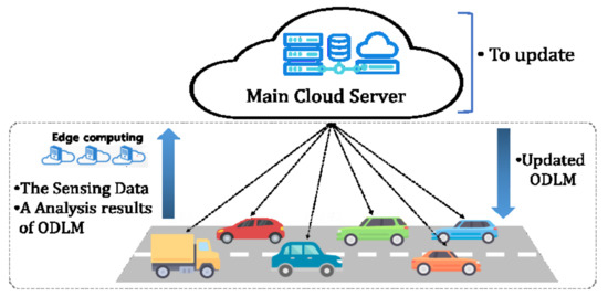
Figure 9. The structure of the Edge Computing based Self-diagnosis Service (ECSS).

The Algorithm 2 shows that of the ECSS and works as follows.

• First, the vehicles transfers the sensing data and the analysis result of the ODLM through the In-VGM to the Main Cloud Server. If there is no analysis result of the ODLM, NULL is used.
• Second, the Main Cloud Server checks that the car having transferred the sensing data and the analysis result of the ODLM is a new car or not.
• Third, if the car is a new car, the Main Cloud Server generates, learns, and stores the ODLM about a new car and transfers the ODLM about the new car to vehicles.
• Fourth, if the car is not a new car, the Main Cloud Server already has the ODLM and learns by applying the sensing data from the vehicles and the analysis result of the ODLM. If the learning is completed, the existing ODLM and the learned ODLM are compared. If the ODLM was changed, the changed contents are transferred to the vehicles.

Algorithm 2. Algorithm of the ECSS

ECSS(Kind of Car, Car’s Sensors Data, ODLM _result){   root <- Kind of Car   data <- Car’s Sensor Data   training <- ODLM _result   if (Is ODLM for root Exist in Cloud) then {     Learning ODLM (data, training)     if(Is ODLM Changed) then {       send ODLM to Car }   }   else{     create ODLM     Learning ODLM (data, training)     save ODLM in Cloud     send ODLM to Car   } }

3.4.2. The V2X Based Accident Notification Service

The VANS informs the adjacent vehicles and infrastructure of the diagnosis result transferred from the Main Cloud Server.

Figure 10 shows the operational process of the VANS.

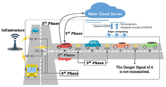
Figure 10. The structure of the V2X based Accident Notification Service (VANS).

• First, the VANS informs the adjacent vehicles of the diagnosis result. According to Figure 10, vehicle A receives the ODLM suitable for itself from the Main Cloud Server. The vehicle analyzes the sensing data by using the received ODLM. If the analysis result decides that the condition of vehicle A is dangerous, the danger alarming message about vehicle A is generated by the VANS. At this time the hop field of the danger alarming message is set as 2. Vehicle A transfers the danger alarming message to an adjacent vehicle B through V2V communication. At this time, the hop field of the danger alarming message becomes 1. The vehicle B having received the danger alarming message transfers it to an adjacent vehicle C through V2V communication. The vehicle C knows the condition of vehicle A by receiving a danger alarming message of vehicle A. At this time, because the hop field of the danger alarming message has 0, vehicle C does not transfer it to other vehicles.
• Second, the VANS informs the adjacent infrastructure of the diagnosis result. According to Figure 10, vehicle A transfers the danger alarming message to the adjacent vehicles and to the adjacent infrastructure at the same time. At this time a hop is not used because a danger alarming message can be transferred to only the adjacent infrastructure. Therefore, the infrastructure having received the danger alarming message of vehicle A transfers the condition of vehicle A to the adjacent vehicles. Vehicle A transfers the sensing data and the analysis result of the ODLM to the Main Cloud Server.

4. The Performance Analysis

This paper proposes an Integrated Self-diagnosis System (ISS) for an Autonomous Vehicle based on an IoT Gateway and Deep Learning. It analyzes the performance of the In-VGM, the ODLM and the DPM.

4.1. The Performance Analysis of the In-VGM

C language is used to analyze the In-VGM performance. If the FlexRay/MOST messages and command are entered in the host PC; CAN message frames are generated in a sending node and transferred to multiple protocols. When 2Byte messages are transferred to CAN, MOST, and FlexRay protocol bus, the message transformation rate and transformation time is compared in the simulation as follows.

In the 1st simulation, the message transformation rate of the existing in-vehicle protocols is compared with that of the In-VGM. 2 Byte messages and 500 s transmission time are used in the simulation. The transmission message is a CAN message and the simulation result is shown in Figure 11.

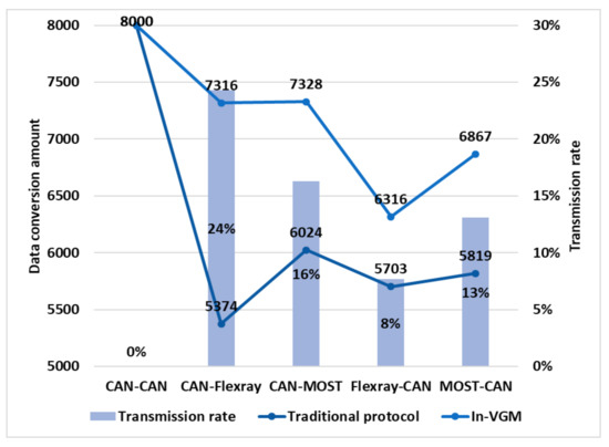
Figure 11. The comparison of the existing in-vehicle protocols with the In-VGM in message transformation rate.

In case a CAN message was transferred to a CAN protocol, the existing in-vehicle protocol and In-VGM have transferred 8000 messages for 500 s and any message transformation was not done. In case a FlexRay message was transferred to a CAN protocol, the In-VGM did more transformations than the existing in-vehicle protocol by 1942 times and its transformation rate is higher than the existing in-vehicle protocol by 24%. In case a MOST message was transferred to a CAN protocol, the In-VGM did more transformations than the existing in-vehicle protocol by 1304 times and its transformation rate is higher than the existing in-vehicle protocol by 16%.

In case a CAN message was transferred to a FlexRay protocol, the In-VGM is higher than the existing in-vehicle protocol by 24% in transformation rate. In case a CAN message was transferred to a MOST protocol, the In-VGM is higher than the existing in-vehicle protocol by 13% in transformation rate. This result was shown because the existing in-vehicle protocol has a disadvantage to put a header in each CAN fragment.

In the 2nd simulation, the transformation time of the existing in-vehicle protocols is compared with that of the In-VGM about 8000 messages and the simulation result is shown in Figure 12.

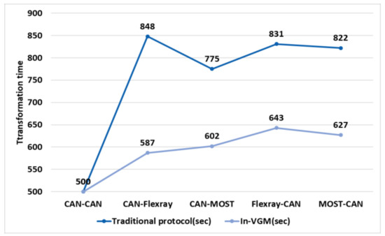
Figure 12. The comparison of the existing in-vehicle protocols with the In-VGM in message transformation time.

It took about 14 min 8 s for the existing in-vehicle protocol to transform 8000 CAN message into the FlexRay protocol and about 12 min 55 s into the MOST protocol. It took about 9 min 47 s for the In-VGM to transform 8000 CAN messages into the FlexRay protocol and about 10 min 2 s into the MOST protocol. It took about 13 min 51 s for the existing in-vehicle protocol to transform a FlexRay message into the CAN protocol, and about 13 min 42 s to transform a MOST message into the CAN protocol. It took about 10 min 43 s for the In-VGM to transform a FlexRay message into the CAN protocol, and about 10 min 27 s to transform a MOST message into the CAN protocol. The In-VGM improves the transmission time by 1.37% compared to the existing in-vehicle protocol.

4.2. The Performance Analysis of the ODLM

To analyze the ODLM performance, the ODLM is compared with the existing Long Short Term Memory (LSTM) and Deep Belief Networks (DBN) in the computation speed and reliability of a Neural Network Model. The Training Data set and Test data are used to analyze the ODLM performance. The ODLM, the LSTM, and the DBN decides the computation speed and reliability with the computation time and error rate occurring in the computation of Test data.

Table 3 shows a control variable value for simulation. The simulation is done three times on the basis of the control variable and compares a Training Dataset learning speed, the response speed of Test Data analysis, and an error rate.

Table 3. A Control Variable Value for Simulation.

Control Variables	Values
the number of Hidden Layers	2
the number of each Hidden Layer Nodes	20
a Learning Rate	0.1
weight (all)	0.2

The 1st experiment compares the average response time by classifying Test data according to the number of sensors and the result is shown in Figure 13.

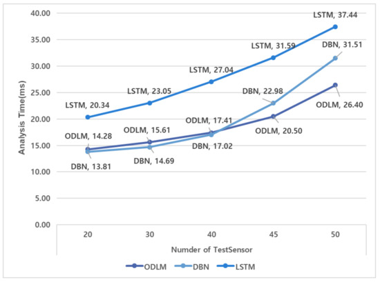
Figure 13. The comparison of the average response time according to the kinds of sensors.

According to Figure 13, the average response time of the ODLM is 14.28 ms in case of 20 sensors, 15.61 ms in case of 30 sensors, and 26.4 ms in case of 50 sensors. The average response time of the DBN is 13.81 ms in case of 20 sensors, 14.69 ms in case of 30 sensors, and 31.51 ms in case of 50 sensors. The average response time of the LSTM is 20.34 ms in case of 20 sensors, 23.05 ms in case of 30 sensors, and 37.44 ms in case of 50 sensors.

Therefore, the average response time of the LSTM is the longest and the more the data, the shorter the average response time of the ODLM.

The 2nd experiment compares the error rate of diagnosis according to the number of Test data sets and the result is shown in Figure 14. In the experiment, the Test data for measurement were randomly selected.

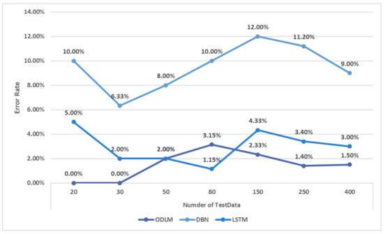
Figure 14. The error rate comparison of diagnosis according to the number of Training Data Set.

According to Figure 14, the ODLM shows an error rate 0% in case of 20 Test data sets, 0% in case of 30 Test data sets, 0% in case of 50 Test data sets and 1.5% in case of 400 Test data sets. The DBN shows an error rate 10% in case of 20 Test data sets, 6.3% in case of 30 Test data sets, 8% in case of 50 Test data sets and 9% in case of 400 Test data sets. The LSTM shows an error rate 5% in case of 20 Test data sets, 2% in case of 30 Test data sets, 2% in case of 50 Test data sets and 3% in case of 400 Test data sets.

Therefore, in the 1st experiment the ODLM improved the analysis speed higher than the DBN by 0.05 s and the LSTM by 0.1 s. In the 2nd experiment, the ODLM showed the lower error rate than the LSTM by 10.5% and the DBN by 1.5%.

4.3. The Performance Analysis of the DPM

The response time and exactness about a self-diagnosis request in the DPM simulation was compared in this section. The DPM simulation is proceeded with 2 PCs (client PC and server PC), but not with a real vehicle according to the increasing number of vehicles. It is assumed that each vehicle has 20 sensors. The sensor data is sent from the client PC to the server PC, and the server PC diagnoses the condition of a vehicle.

The 1st experiment is processed as follows.

Figure 15 shows an average response time of a self-diagnosis request. It takes 1.305 ms for the DPM to reply to the request of about 20 vehicles, 2.175 ms of 30 vehicles, 4.65 ms of 50 vehicles, 14.78 ms of 800 vehicles, and 19.71 ms of roughly 1200 vehicles. It takes 0.48 ms for the existing Cloud system to reply to the request of about 20 vehicles, 1.14 ms of 30 vehicles, 3.21 ms of 50 vehicles, 17.61 ms of 800 vehicles, 24.26 ms of 1200 vehicles. Therefore, it shows that the more vehicles there are, the more efficient the DPM is over the existing Cloud system.

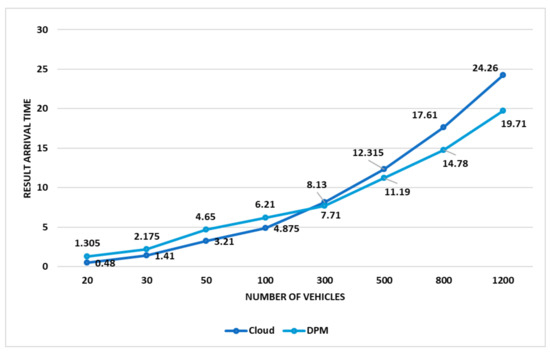
Figure 15. The comparison of an average response time about a self-diagnosis request.

The 2nd simulation shows the exactness comparison about a self-diagnosis request and reply.

Figure 16 shows the experimental result of error times about a self-diagnosis request and reply between the DPM and the existing Cloud system. In case of transferring a request message to 100 vehicles or fewer, both the existing Cloud system and the DPM had 0 response error or 1 response error. The existing Cloud system had 3 response errors in the case of transferring a request message to 300 vehicles, 5 response errors to 500 vehicles, 10 response errors to 800 vehicles, and 13 response errors to 1200 vehicles. Therefore, the response exactness of the existing Cloud system was analyzed as 98%.

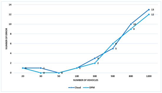
Figure 16. The comparison result of error times about a self-diagnosis request and reply.

The DPM proposed in this paper had 2 response errors in the case of transferring a request message to 300 vehicles, 6 response errors to 500 vehicles, 9 response errors to 800 vehicles, and 12 response errors to 1200 vehicles. Therefore, the response exactness of the DPM was analyzed as 99% and the DPM shows that the larger number of vehicles there is, the higher the response speed.

5. Conclusions

This paper proposes “An Integrated Self-diagnosis System (ISS) for an Autonomous Vehicle based on an IoT Gateway and Deep Learning” which collects information from the sensors of an autonomous vehicle, diagnoses itself and the influence between parts by using Deep Learning and informs drivers of the result. In three experiments, the In-VGM improves the transmission time by 1.37% compared to the existing in-vehicle protocol and the ODLM improved analysis speed was higher than the DBN by 0.05 s and the LSTM by 0.1 s. The response exactness of the DPM was analyzed as 99%. This means that the proposed ISS is better than existing vehicle diagnostic methods. The ISS has some advantages. It guarantees compatibility by transforming different types of data from different communication protocols into the same type of data. Also, it improves the response speed processing sensor data and reduces overhead by using Edge Computing. Lastly, it prevents a chain collision by informing adjacent vehicles and infrastructures of accidents and dangers in advance.

In this paper, a controlled environment is used with 50 limited sensors and 5 Hidden Layers, but in future work more sensors and hidden layers will be applied to real vehicles, and not PCs, to achieve a precise experiment.

References

- Schweber, B. The Autonomous Car: A Diverse Array of Sensors Drives Navigation, Driving, and Performance. Available online: https://www.mouser.com/applications/autonomous-car-sensors-drive-performance/ (accessed on 10 January 2018).
- Miller, D. Autonomous Vehicles: What Are the Security Risks? 2014. Available online: https://www.covisint.com/blog/autonomous-vehicles-what-are-the-security-risks/ (accessed on 10 January 2018).
- Black, T.G. Diagnosis and Repair for Autonomous Vehicles. 2014. Available online: http://www.freepatentsonline.com/8874305.html (accessed on 11 January 2018).
- Xie, G.; Zeng, G.; Kurachi, R.; Takada, H.; Li, Z.; Li, R.; Li, K. WCRT Analysis of CAN Messages in Gateway-Integrated In-Vehicle Networks. IEEE Trans. Veh. Technol. 2017, 66, 9623–9637. [Google Scholar] [CrossRef]
- Wong, W. Design FAQs: FlexRay. Electron. Des. 2006, 54, 30. [Google Scholar]
- Li, Z.; Jing, H.; Liu, Z. Design of Application Layer Software and Interface Circuit for the MOST Network in Vehicle. In Proceedings of the Proceedings of the 32nd Chinese Control Conference, Xi’an, China, 26–28 July 2013; pp. 7720–7725. [Google Scholar]
- Lee, T.; Kuo, C.; Lin, I. High performance CAN/FlexRay gateway design for In-Vehicle network. Dependable and Secure Computing. In Proceedings of the 2017 IEEE Conference on Dependable and Secure Computing, Taipei, Taiwan, 7–10 August 2017; pp. 240–242. [Google Scholar]
- Dong, Z.; Piao, Z.; Jang, I.; Chung, J.; Lee, C. Design of FlexRay-MOST gateway using static segments and control messages. In Proceedings of the 2012 IEEE International Symposium on Circuits and Systems (ISCAS), Seoul, Korea, 20–23 May 2012; pp. 536–539. [Google Scholar]
- Seo, S.H.; Kim, J.H.; Moon, T.Y.; Hwang, S.H.; Kwon, K.H.; Jeon, J.W. A Reliable Gateway for In-vehicle Networks. In Proceedings of the 17th World Congress The International Federation of Automatic Control, Seoul, Korea, 6–11 July 2008; Volume 41, pp. 12081–12086. [Google Scholar]
- Kim, J.H.; Seo, S.; Hai, N.; Cheon, B.M.; Lee, Y.S.; Jeon, J.W. Gateway Framework for In-Vehicle Networks Based on CAN, FlexRay, and Ethernet. IEEE Trans. Veh. Technol. 2014, 64, 4472–4486. [Google Scholar] [CrossRef]
- Yang, J.; Wang, J.; Wan, L.; Liu, X. Vehicle networking data-upload strategy based on mobile cloud services. EURASIP J. Embed. Syst. 2016, 22. [Google Scholar] [CrossRef]
- Thiele, D.; Schlatow, J.; Axer, P.; Ernst, R. Formal timing analysis of CAN-to-Ethernet gateway strategies in automotive networks. Real-Time Syst. 2016, 52, 88–112. [Google Scholar] [CrossRef]
- Kim, M.; Lee, S.; Lee, K. Performance Evaluation of Node-mapping-based FlexRay-CAN Gateway for In-Vehicle Networking System. Intell. Autom. Soft Comput. 2015, 21, 251–263. [Google Scholar] [CrossRef]
- Lee, Y.S.; Kim, J.H.; Jeon, J.W. FlexRay and Ethernet AVB Synchronization for High QoS Automotive Gateway. IEEE Trans. Veh. Technol. 2016, 66, 5737–5751. [Google Scholar] [CrossRef]
- Ju, K.; Chen, L.; Wei, H.; Chen, K. An Efficient Gateway Discovery Algorithm with Delay Guarantee for VANET-3G Heterogeneous Networks. Wirel. Pers. Commun. 2014, 77, 2019–2036. [Google Scholar] [CrossRef]
- Aljeri, N.; Abrougui, K.; Almulla, M.; Boukerche, A. A reliable quality of service aware fault tolerant gateway discovery protocol for vehicular networks. Wirel. Commun. Mob. Comput. 2015, 15, 1485–1495. [Google Scholar] [CrossRef]
- Seo, S.; Kim, J.; Hwang, S.; Kwon, K.H.; Jeon, J.W. A reliable gateway for in-vehicle networks based on LIN, CAN, and FlexRay. ACM Trans. Embed. Comput. Syst. 2012, 11, 1–24. [Google Scholar] [CrossRef]
- An, H.S.; Jeon, J.W. Analysis of CAN FD to CAN message routing method for CAN FD and CAN gateway. In Proceedings of the 2017 17th International Conference on Control, Automation and Systems (ICCAS), Jeju, Korea, 18–21 October 2017. [Google Scholar]
- Seo, H.S.; Kim, B.C.; Park, P.S.; Lee, C.D.; Lee, S.S. Design and implementation of a UPnP-can gateway for automotive environments. Int. J. Autom. Technol. 2013, 14, 91–99. [Google Scholar] [CrossRef]
- Wang, L.; Wang, L.; Liu, W.; Zhang, Y. Research on fault diagnosis system of electric vehicle power battery based on OBD technology. In Proceedings of the 2017 International Conference on Circuits Devices and Systems (ICCDS), Chengdu, China, 5–8 September 2017; pp. 95–99. [Google Scholar]
- Khorsravinia, K.; Hassan, M.K.; Rahman, R.Z.A.; Al-Haddad, S.A.R. Integrated OBD-II and mobile application for electric vehicle (EV) monitoring system. In Proceedings of the 2017 IEEE 2nd International Conference on Automatic Control and Intelligent Systems (I2CACIS), Kota Kinabalu, Malaysia, 21 October 2017; pp. 202–206. [Google Scholar]
- Chen, S.; Liu, W.; Tsai, J.; Hung, I. Vehicle fuel pump service life evaluation using on-board diagnostic (OBD) data. In Proceedings of the 2016 International Conference on Orange Technologies (ICOT), Melbourne, VIC, Australia, 18–20 December 2016; pp. 84–87. [Google Scholar]
- Zhang, H.; Li, W. A new method of sensor fault diagnosis based on a wavelet packet neural network for Hybrid electric vehicles. In Proceedings of the 2016 9th International Congress on Image and Signal Processing, BioMedical Engineering and Informatics (CISP-BMEI), Datong, China, 15–17 October 2016; pp. 1143–1147. [Google Scholar]
- Zhang, Z.; He, H.; Zhou, N. A neural network-based method with data preprocess for fault diagnosis of drive system in battery electric vehicles. In Proceedings of the 2017 Chinese Automation Congress (CAC), Jinan, China, 20–22 October 2017; pp. 4128–4133. [Google Scholar]
- Moosavi, S.S.; Djerdir, A.; Ait-Amirat, Y.; Khaburi, D.A.; N’Diaye, A. Artificial neural network-based fault diagnosis in the AC–DC converter of the power supply of series hybrid electric vehicle. IET Electr. Syst. Transp. 2016, 6, 96–106. [Google Scholar] [CrossRef]
- Chuang, C.; Wei, Z.; Zhifu, W.; Zhi, L. The diagnosis method of stator winding faults in PMSMs based on SOM neural networks. Energy Procedia 2017, 105, 2295–2301. [Google Scholar] [CrossRef]
- Yurii, K.; Liudmila, G. Application of Artificial Neural Networks in Vehicles’ Design Self-Diagnostic Systems for Safety Reasons. Transp. Res. Procedia 2017, 20, 283–287. [Google Scholar] [CrossRef]
- Chunyan, W.; Wanzhong, Z.; Zhongkai, L.; Qi, G.; Ke, D. Decoupling control of vehicle chassis system based on neural network inverse system. Mech. Syst. Signal Process. 2017, 106, 176–197. [Google Scholar]
- Chu, W.; Liu, Y.; Shen, C.; Cai, D.; Hua, X. Multi-Task Vehicle Detection With Region-of-Interest Voting. IEEE Trans. Image Process. 2018, 27, 432–441. [Google Scholar] [CrossRef] [PubMed]
- Liu, W.; Zhang, M.; Luo, Z.; Cai, Y. An Ensemble Deep Learning Method for Vehicle Type Classification on Visual Traffic Surveillance Sensors. IEEE Access 2017, 5, 24417–24425. [Google Scholar] [CrossRef]
- Tan, D.; Chen, W.; Wang, H. On the Use of Monte-Carlo Simulation and Deep Fourier Neural Network in Lane Departure Warning. IEEE Intell. Transp. Syst. Mag. 2017, 9, 76–90. [Google Scholar] [CrossRef]
- Chen, C.; Hongyu, X.; Tie, Q.; Cong, W.; Yang, Z.; Victorm, C. A rear-end collision prediction scheme based on deep learning in the Internet of Vehicles. J. Parallel Distrib. Comput. 2017, 117, 192–204. [Google Scholar] [CrossRef]
- Wang, H.; Cai, Y.; Chen, X.; Chen, L. Night-Time Vehicle Sensing in Far Infrared Image with Deep Learning. J. Sens. 2016, 2016, 3403451. [Google Scholar] [CrossRef]
- George, L.; Yongpil, Y.; Georgia, S.; Tuan, V.; Ryan, H. Computation offloading of a vehicle’s continuous intrusion detection workload for energy efficiency and performance. Simul. Model. Pract. Theory 2016, 73, 83–94. [Google Scholar]
- Gao, Y.; Lee, H.J. Local Tiled Deep Networks for Recognition of Vehicle Make and Model. Sensors 2016, 16, 226. [Google Scholar] [CrossRef] [PubMed]
- Liujuan, C.; Qilin, J.; Ming, C.; Cheng, W. Robust vehicle detection by combining deep features with exemplar classification. Neurocomputing 2016, 215, 225–231. [Google Scholar]
- Meng, Z.; Pan, J.-S. Monkey King Evolution: A new memetic evolutionary algorithm and its application in vehicle fuel consumption optimization. Knowl. Based Syst. 2016, 97, 144–157. [Google Scholar] [CrossRef]
- Zhao, D.; Chen, Y.; Lv, L. Deep Reinforcement Learning With Visual Attention for Vehicle Classification. IEEE Trans. Cognit. Dev. Syst. 2016, 9–4, 356–367. [Google Scholar] [CrossRef]
- Gonzalez, J.P.N.; Castañon, L.E.G.; Rabhi, A.; El Hajjaji, A.; Morales-Menendez, R. Vehicle Fault Detection and Diagnosis combining AANN and ANFI. IFAC Proc. 2009, 42, 1079–1084. [Google Scholar] [CrossRef]
- Yang, S.; Cao, Y.; Peng, Z.; Wen, G.; Guo, K. Distributed formation control of nonholonomic autonomous vehicle via RBF neural network. Mech. Syst. Signal Process. 2017, 87, 81–95. [Google Scholar] [CrossRef]
- Luo, X.C.; Shen, R.; Hu, J.; Deng, J.; Hu, L.; Guan, Q. A Deep Convolution Neural Network Model for Vehicle Recognition and Face Recognition. Procedia Comput. Sci. 2017, 107, 715–720. [Google Scholar] [CrossRef]
- Glowacz, A. Acoustic based fault diagnosis of three-phase induction motoer. Appl. Acoust. 2018, 137, 82–89. [Google Scholar] [CrossRef]
- Praveenkumar, T.; Sabhrish, B.; Saimurugen, M.; Ramachandran, K.I. Pattern recognition based on-line vibration monitoring system for fault diagnosis of automobile gearbox. Measurement 2018, 114, 233–242. [Google Scholar] [CrossRef]
- Ganovska, B.; Molitoris, M.; Hosovsky, A.; Pitel, J.; Krolczyk, J.B.; Ruggierio, A.; Krolczyk, G.M.; Hloch, S. Design of the model for the on-line control of the AWJ technology based on neural networks. Indian J. Eng. Mater. Sci. 2016, 23, 279–287. [Google Scholar]
- Hu, Z.; Su, J.; Vladimir, J.; Orest, K.; Mykola, M.; Roman, K.; Taras, S. Data Science Applications to Improve Accuracy of Thermocouples. In Proceedings of the 2016 IEEE 8th International Conference On Intelligent Systems, Sofia, Bulgaria, 4–6 September 2016; pp. 180–188. [Google Scholar]
- Kamada, S.; Ichimura, T. Knowledge extracted from recurrent deep belief network for real time deterministic control, Systems, Man, and Cybernetics (SMC). In Proceedings of the 2017 IEEE International Conference on Systems, Man, and Cybernetics (SMC), Banff, AB, Canada, 5–8 October 2017; pp. 825–830. [Google Scholar]
- Lehner, B.; Widmer, G.; Bock, S. A low-latency, real-time-capable singing voice detection method with LSTM recurrent neural networks. In Proceedings of the 23rd European Signal Processing Conference (EUSIPCO), Nice, France, 31 Augudte–4 September 2015; pp. 21–25. [Google Scholar]
© 2018 by the authors. Licensee MDPI, Basel, Switzerland. This article is an open access article distributed under the terms and conditions of the Creative Commons Attribution (CC BY) license (http://creativecommons.org/licenses/by/4.0/).