Abstract
Convolutional neural networks (CNNs) with log-mel audio representation and CNN-based end-to-end learning have both been used for environmental event sound recognition (ESC). However, log-mel features can be complemented by features learned from the raw audio waveform with an effective fusion method. In this paper, we first propose a novel stacked CNN model with multiple convolutional layers of decreasing filter sizes to improve the performance of CNN models with either log-mel feature input or raw waveform input. These two models are then combined using the Dempster–Shafer (DS) evidence theory to build the ensemble DS-CNN model for ESC. Our experiments over three public datasets showed that our method could achieve much higher performance in environmental sound recognition than other CNN models with the same types of input features. This is achieved by exploiting the complementarity of the model based on log-mel feature input and the model based on learning features directly from raw waveforms.
1. Introduction
In recent years, while research in auditory recognition has often been focusing on automatic speech recognition (ASR), music classification [1], and acoustic scene classification (ASC), the environmental event sound recognition (ESC) problem has also received increasing attention from the research community with popular applications in audio surveillance systems [2] and noise mitigation [3]. In the ESC problem or sound event detection problem, the goal is to recognize the event type of a specific sound, such as a dog bark, car horn, or engine. These sound events include various daily audio events with chaotic and diverse structure [4] and can be categorized into three groups: single sounds such as a mouse-click, repeated discrete sounds such as clapping hands or typing on a keyboard, and steady continuous sounds such as the sound of a vacuum cleaner or engine [5]. The sound event classification problem is sometimes confused with the related ASC problem, in which an input sound is required to be classified into different acoustic scenes. Each acoustic scene may contain a collection of sound events involved in the surrounding environment. For example, a ‘bus’ scene may be identified from frequently occurring sound events such as acceleration, braking, passenger announcements, and door opening sounds, while the engine and other people’s conversations exist in the background [6]. Here, we limit the scope of our study to the recognition of specific or individual sound events in an environment.
A variety of traditional audio features such as zero-crossing, mel frequency cepstral coefficients [7,8,9], and wavelet transformation have been used to represent sound features for an environmental sound event. Traditional machine learning algorithms such as K nearest neighbor, support vector machines, and Gaussian mixture models have been applied to classify the sound [10,11,12,13]. With the popularity of deep learning, deep neural networks [14,15,16,17] have also been proposed to solve the sound event recognition problem in an environment. In particular, the convolutional neural network is regarded as being most suitable for this problem [18,19], due to its capability to capture time and frequency features when applied to spectrogram-like inputs. Three different ways of applying CNNs to sound event recognition have been proposed. The first approach is to use the CNN as the classifier with log-mel features as the input [4,19], which are extracted from environmental sound. We refer to this method as logmel-CNN. The second CNN approach learns to classify the sound directly from raw waveforms without feature engineering. These raw-CNN methods use CNNs to extract audio features from raw wave signals for ESC [20,21,22,23]. Tokozume [5] proposed an end-to-end system (EnvNet) to classify raw waveform signals using two convolution layers. The accuracy of their method was 5.1% higher than that of the models using static log-mel features. The third hybrid CNN approach combines raw-CNN and logmel-CNN methods for this task [5] using an average fusion method and achieved a better performance than that of either method alone.
Current approaches have the following limitations: (1) since the log-mel feature was originally designed for ASR rather than for ESC tasks, it may fail to capture some information of the audio events that may be critical for further improved performance; (2) currently, end-to-end recognition models with feature learning cannot surpass CNN models with static log-mel and delta log-mel features in terms of recognition accuracy. This indicates that new neural network models are needed to achieve high-performance ESC; (3) the current average fusion method can reflect overall prediction results of the hybrid models, but has the drawback of neglecting the tendency of individual models. It can also be easily affected by extreme values, leading to recognition errors.
To address the obstacles for ESC as discussed above, we propose a new stacked convolutional neural network model to improve the recognition performance of both the logmel-CNN and raw-CNN models. A new Dempster-Shafer (DS) evidence theory-based fusion algorithm is also proposed to exploit the synergistic capabilities of the raw-CNN and logmel-CNN approaches, which achieved better fusion performance than the average fusion approach. DS evidence theory, as a classical fusion algorithm, has the ability to consider the basic credibility distribution (prediction results) of several models to achieve better fusion, and has been widely used in multisource information fusion for recognition, which has achieved favorable results [24,25,26,27,28].
The main contributions of this paper are as follows:
- (1)
- We proposed a five-layer stacked CNN network for sound event recognition based on a special convolutional filter configuration with decreasing filter sizes and static and delta log-mel input features. The test results from three datasets, ESC-10, ESC-50 [1], and Urbansound8k [29], indicated that the recognition performance of our model is higher than those of previous logmel-CNN models including Picazk [4], Salamon and Bello [19], and EnvNet [5].
- (2)
- We designed an end-to-end stacked CNN model for sound event recognition from raw waveforms without feature engineering. It has a special two-layer feature extraction convolution layer and convolutional filter configuration to directly learn features from raw waveforms. Our models achieve a 2% and 16% improvement in recognition accuracy on the datasets of ESC-50 and Urbansound8k [29], respectively, compared to the existing top end-to-end model EnvNet [5] and the 18-layer convolutional neural network [22].
- (3)
- We developed a novel ensemble environmental event sound recognition model, DS-CNN, by fusing logmel-CNN and end-to-end raw-CNN models using DS evidence theory to exploit raw waveform features as well as the log-mel features. The experimental result indicated that the recognition accuracy of the DS-CNN had surpassed the recognition accuracy of human and other mainstream algorithms over the ESC-50 dataset and is better than other simple averaging and product of probability fusion methods. To our knowledge, this is the first instance of applying DS fusion to the environmental sound recognition problem with improved recognition performance.
The remaining structure of this paper is as follows. Section 2 describes related works on environmental sound recognition. In Section 3, we first present the overall framework of the DS environmental recognition model. Then, we introduce the method of feature extraction and the network architecture. The detailed description of the experimental dataset and results are described in Section 4. Finally, we draw conclusions about our work in Section 5.
2. Related Work
In recent years, due to the success of deep learning in computer vision, speech recognition, and other related areas, deep neural network models such as CNN and Long Short-Term Memory (LSTM) have been applied to solve the ESC problem. These methods can be further divided by the input features they use.
The log-mel feature of audio signals is regarded as one of the most powerful features for audio recognition [5], due to its consideration of human auditory perception. It is calculated for each frame of the sound and represents the magnitude of each frequency area [30]. A log-mel feature map can be generated by arranging the log-mel features of each frame along the time axis. Since the feature map of log-mel has locality in both the time and frequency, researchers take the convolutional layer as the basic component of the classification model and classify the feature in a similar way to image classification. This method was proposed by Piczak [4] and was first applied in environmental sound classification. He extracted log-mel features in each frame and calculated the first temporal derivative of log-mel to obtain the delta log-mel feature. Then, he treated the two-dimensional feature map constituted by static log-mel and delta log-mel as a two-channel input to CNN for classification, similar to how the RGB images are used in image classification [31]. Salamon and Bello [19] used a log-mel feature map as a two-channel input for the network classification model, which was composed of three convolutional layers and one fully connected layer. In addition, he adopted a data augmentation technique to increase the variation of training data to efficiently train the network. This increased the accuracy by 6% on the Urbansound8k dataset compared to Piczak’s approach [4].
Several attempts have been made to achieve the learning of features automatically from raw waveforms for ESC [32,33,34,35,36]. However, the classification accuracy was not as good as the models using log-mel features [5]. End-to-end learning of audio features has also been explored for speech recognition. Motivated by Hoshen [20], Tara etc. [21] took the first convolutional layer as a finite impulse response filter bank followed by a nonlinearity mapping layer and applied it directly to the one-dimensional raw waveform. The first convolutional layer is called the time convolution layer (tconv), which is used to reduce changes in time domain, while the second convolution layer (fconv) is used to reduce frequency spectrum changes of the feature vectors and maintain locality features in frequency. The three LSTM layers and two Deep Neural Networks (DNN) layers are used for classification. Trained over 2000 h of speech, the recognition rate of their models, using raw waveforms as input, first matches the performance of the model with the log-mel feature on both voice search tasks. Based on this research, Dai [22] proposed to use deep convolutional neural networks to optimize over long sequences of raw audio waveforms. The experimental results indicated that with up to 18 convolutional layers, the classification accuracy of the CNN model can outperform the model with three convolutional layers by 15%. It could match the performance of CNN models with log-mel features. When the number of convolutional layers reached 34, it could process long raw audio waveforms effectively.
In this paper, our goal is to improve the recognition performance of the log-mel feature-based prediction model by proposing stacked convolutional neural network models using logmel-CNN and raw-CNN, and then build a hybrid ESC recognition model using DS evidence theory to further improve recognition accuracy of environmental sounds.
3. DS-CNN: Sound Recognition Model Based on CNN and DS Evidence Theory
Previous studies [5] have found that log-mel and raw features can capture different patterns of a given sound. Therefore, recognition models based on these two feature inputs can be combined to exploit the complementary relationships for further improvement in recognition performance. Here, we propose an information fusion method to combine the prediction results of MelNet and RawNet using DS evidence theory [37], which is an uncertainty reasoning theory first proposed by Dempstert and further developed by Shafe [38].
Our DS-CNN sound recognition model is shown in Figure 1. It consists of three parts: the logmel-CNN, raw-CNN, and DS evidence theory-based fusion of their predictions. We refer to these two convolutional neural network models as MelNet and RawNet, respectively. The MelNet is divided into two parts: the log-mel feature extraction module Figure 1b and the recognition module (Figure 1(c1)). The architecture of the RawNet is shown in bottom part of Figure 1, which consists of two parts: feature learning module (Figure 1a) and recognition module (Figure 1(c2)).
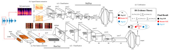
Figure 1.
The overall framework of the Dempster-Shafer sound recognition system. (a) shows the RawNet feature learning module; (b) shows the MelNet log-mel feature extraction module; (c1) shows the recognition module in MelNet; (c2) shows the recognition module in RawNet.
In Section 3.1, we show the detailed architecture of these two CNNs used in our system. In Section 3.2, we will describe the principle of DS evidence theory and the combination method used in the task of sound recognition. The justification of the architecture and parameter settings is detailed in Section 5.
3.1. Network Architectures
3.1.1. Feature Learning Module in RawNet
The feature learning module in RawNet (Figure 1a) contains two convolutional layers (before the pooling layer) to extract features from the raw waveform input with two dimensions. Each convolutional layer with filters of small receptive fields is functionally similar to a bandpass filter bank. Each layer has 40 filters, generating a two-dimensional vector, which can be thought of as the components that we extract from a log-scaled mel-spectrogram input. It covers the audible frequency range (0–22,050 Hz) of the sound segment (about 1 s). Here, each filter corresponds to a frequency characteristic. The receptive field is set as (1,8) in both convolution layers, and the stride is set as (1,1) in time series. The small filter size is set according to the experimental results of EnvNet [5], which demonstrated that the CNN model can extract local features of various time scales hierarchically by using multiconvolutional layers with small receptive fields. The input shape and the parameters of the first two convolutional layers are as in Table 1.

Table 1.
Parameters of the feature learning module in RawNet.
The output of these two convolutional layers is noted as the “time-frequency” feature representation. We then apply no-overlapping max pooling to the output of the convolutional layers with a pooling size of 128. Then, the output of the pool matrix is of size 1 × 160 × 40 (frequency × time × channel), which is then reshaped to 40 × 160 × 1 in order to convolve them in both frequency and time. Finally, the three-dimensional matrix 40 × 160 × 1 is fed into the convolutional layer “conv3” to do classification.
3.1.2. Log-Mel Feature Extraction in MelNet
As for the log-mel feature, we use the same feature extraction method as Piczak [4]. We use the librosa Python library to extract the log-scaled mel-spectrogram features with 60 bands to cover the frequency range (0–22,050 Hz) of the sound segments. At the same time, the sound segments are divided into 41 frames with an overlap of 50%, with each frame being about 23 ms. Through these steps, we can represent the static log-scaled mel-spectrogram feature on each segment as a 60 × 40 × 1 matrix corresponding to frequency × time × channel. In addition, we calculate the first temporal derivative of log-mel on each frame to obtain the delta log-scaled mel-spectrogram feature, which is used as the second channel of input. Finally, the dimension of the extracted log-scaled mel-spectrogram feature maps is 60 × 41 × 2.
3.1.3. Structure of the RawNet and MelNet
As shown in parts (c1) and (c2) of Figure 1, the recognition modules of both RawNet and MelNet contain five convolutional layers and a fully connected layer. The architecture and parameters of the network are as follows:
- L1: The first layer of the network uses 24 filters with a receptive field of (6,6) and stride of (1,1). ReLU is used as the activation function. The small receptive field of (6,6) here is used to learn smaller and more local “time-frequency” characteristics of sound segments.
- L2: motivated by the VGG network [39], the second layer uses the same parameters as the first layer, which uses 24 filters with a receptive field of (6,6) and stride of (1,1). At the same time, ReLU is used as the activation function. The nonlinear transformation of the output from previous convolutional layer enables the network to learn high-level features.
- L3: the third layer of the network uses 48 filters with a receptive field of (5,5) and stride of (2,2). This is followed by an ReLU activation function.
- L4: the fourth layer uses 48 filters with a receptive field of (5,5) and stride of (2,2). ReLU is used as the activation function.
- L5: the fourth layer uses 64 filters with a receptive field of (4,4) and stride of (2,2). ReLU is used as the activation function.
- L6: the sixth layer is a fully connected layer with 200 hidden units, followed by a ReLU activation function.
- L7: the output is 10 or 50 units, which is followed by a softmax activation function.
Differently from the standard CNN configuration, we do not adopt a max-pooling layer after the convolutional layers of the recognition modules in either RawNet or MelNet to keep more information. Instead, a Batch normalization layer is used to accelerate and improve the learning process of deep neural networks. In addition, the Batch normalization layer is followed by a fully connected layer. For the RawNet model, we applied a 0.5 dropout probability for the fully connected layer to prevent overfitting. We used a learning decay scheme to train the models. In order to investigate the effect of the stacked CNN architecture and parameters on classification performance, we conducted extensive experiments in Section 4.3.
3.2. DS Evidence Theory-Based Prediction Fusion
The most basic concept of DS evidence theory is to establish a frame of discernment, , and a finite set of elements , where n is the number of elements. Each element is incompatible and independent. The power set of is . In the DS theory of evidence, if the elements in the frame of discernment satisfy the exclusiveness condition, when element is assigned by the basic probability assignment function , the mapping of the power set to the , satisfies:
- (1)
- , indicating that the probability of an impossible event is 0.
- (2)
- , indicating that the total probability of the event is 1.
is referred to as the basic probability assignment (BPA) of the element , reflecting the degree of trust in the element itself.
Here, each class of sounds in the dataset can be regarded as one element in under the frame of discernment ( for ESC-10 and Urbansound8k; for ESC-50). All elements are exclusive and independent. Meanwhile, the output values of the activation functions (softmax) of the MelNet and the RawNet models are used as the basic probability assignments and , respectively, under the same frame of discernment, . and meet the following conditions:
Then, we use an orthogonal operation to effectively synthesize the basic probability assignments of and generated by these two models. For any , the fusing formula is as follows:
is a coefficient used to measure the degree of conflict between the various evidences of fusion. The output value is also a basic probability assignment and satisfies , which is called the comprehensive probability assignment of and . It is a normalization constant. We use as the final prediction result of the fusion.
4. Experiment Results
4.1. Test Datasets
We used three datasets, ESC-10, ESC-50, and Urbansound8k, to train and evaluate our ESC prediction models. ESC-50 consists of 2000 audio files with environmental sound events of 50 equally balanced categories. Each file contains 5 s of sound. The ESC-10 dataset is selected from ESC-50, which contains 400 recordings and can be divided into 10 categories: dog barking, rain, sea waves, baby crying, clock ticking, person sneezing, helicopter, chainsaw, rooster, and file crackling. Urbansound8k contains 10 classes of 8732 short audio files of urban sound sources.
4.2. Data Preparation
We convert all sound files to monaural wav files with a sampling rate of 22,050 Hz. Differently from other standard methods, we did not remove the silent section from the whole 5-s sound to preserve the integrity of the original audio. Then, we follow a standard data augmentation procedure [5]. We set the window size to 1024 (about 46 ms), take 1/2 of the window size as the hop size, and split it into 50% overlapping segments. The length of each sound segment is 20,480 (about 1 ms). We reshape the raw waveform segment from a one-dimensional form (20,480) into a two-dimensional matrix (1, 20,480) with one channel so that it matches the commonly used 2D filters in Tensorflow. When we train the network, we randomly select these segments from the original training audio and input them into the prediction models. At each epoch, we choose different segments of the audio, but use the same training label, regardless of the selected segments. In the test phase, we input multiple segments of the audio file into the prediction network and perform a majority voting of the output prediction results for classification.
4.3. Experiment Setup
The models were evaluated with a K-fold cross-validation scheme in all datasets (K = 5 for ESC-10 and ESC-50, K = 10 for UrbanSound8k). The single training fold is used as the validation set for parameter tuning, following the approach in [19]. We performed cross-validation five times over the three datasets to evaluate our networks with log-mel features, with raw features, and with both for the hybrid DS-CNN method.
4.4. Experimental Result
We perform a five-fold cross validation in ESC and a 10-fold cross validation in Urbansound8k to evaluate our model with log-mel feature input. We compared our MelNet model with existing logmel-CNN models as reported by Piczak [4], Tokozume and Harada [5], and Salamon and Bello [19]. The results are presented in Table 2. First of all, with the ESC-50 dataset, the accuracy of our model (MelNet) is 81.1%, which is much higher than the 64.5% of the Piczak [4] model and the 66.5% of the static-delta logmel-CNN proposed by Tokozume and Harada [5]. Our algorithm performance is just slightly lower than the 81.3%, the human recognition accuracy. This is the first time that the recognition accuracy has reached over 80% using the logmel-CNN learning method on the ESC-50 dataset.
Table 2.
Comparison of recognition accuracy with other models on evaluated datasets.
On the ESC-10 dataset, the accuracy of MelNet reaches 91.4%, which is 9.9% and 4.5% higher than the accuracy (81.5%) of Piczak’s [4] logmel-CNN model and that of the logmel-CNN + BN model (86.8%), respectively. Finally, we evaluated the algorithms on the Urbansound8k dataset. The accuracy of MelNet is 90.2%, which is also higher than the 73.7% accuracy of Piczak [4] and the 79% of Salamon and Bello [19]. These results indicate that our five-layer stacked convolutional neural network has achieved significant improvement in sound recognition with the log-mel features as input. To our knowledge, our MelNet is the most effective model for environmental sound recognition using log-mel as the feature.
Next, we evaluated the performance of our RawNet CNN model that takes raw waveforms as the input of the network. By using simpler features, convolutional neural networks work by extracting feature representation from raw audio signals and then do recognition, implementing an end-to-end way for sound recognition. We evaluated the recognition performance of the RawNet on three datasets and compared the test results with the performance of existing models. On the ESC-50 dataset, our accuracy reached 66.2%, slightly higher than the 64% of Tokozume and Harada’s [5] method. On the Urbansound8k dataset, our accuracy reached 87.7%, which is higher than that achieved by Dai [22], with 71.68% accuracy. This indicates that our model structure also has a better recognition accuracy for ESC with raw waveform input.
Finally, we evaluated the performance of the DS-CNN, which combines the CNN model based on the log-mel feature input and raw-CNN using the raw waveform feature as the input. We used the ESC-50 and Urbansound8k datasets to compare the recognition performance before and after the model fusion. We trained the RawNet and MelNet models in a standard way. Then, each segment in the sound file was predicted, which output the softmax values. These two softmax values of the two models were assigned as the basic probability assignment m1, m2. Then, m1 and m2 are fused by the orthogonal operation. In this experiment, we still used the k-fold cross validation (k = 5 for ESC-50, k = 10 for Urbansound8k) to evaluate the performance of our DS-CNN method.
The experimental results of the DS-CNN on the ESC-50 and Urbansound8k datasets are shown in Table 2. We find that when the DS evidence theory is used to merge these two models, the accuracy has increased by 2% compared with the logmel-CNN method, reaching 83.1%, which is higher than the recognition accuracy (81.3%) of the human. This demonstrates that the raw waveform feature is capable of complementing the log-mel feature in ESC by providing information that is otherwise neglected by the log-mel feature. On the ESC-50 dataset, the accuracy of DS-CNN, designed by us, is 12.1% higher than that of the ensemble model proposed by Tokozume [5], which proves the superiority of our model in dealing with the environmental sound event recognition.
In order to further demonstrate whether the DS-CNN outperforms RawNet and MelNet in a statistically significant way, we added the experimental results from paired accuracy statistics and applied a paired sample t-test. Table 3 shows the performance achieved by the three models with ESC-50. The accuracy scores of the single models are 65.7% and 81.09%, obtained by RawNet and MelNet, respectively. Moreover, for the fusion model (DS-CNN), the accuracy is 83.09%. The results demonstrate that the fusion model (DS-CNN) outperforms both RawNet and MelNet.
Table 3.
Statistics of accuracy achieved by the three models.
The results for the two paired sample t-tests of accuracies obtained by DS-CNN, RawNet, and MelNet are summarized in Table 4. On average, the DS-CNN has improved the performances of RawNet and MelNet by 18% and 2%, respectively. The two-tailed p-values approach zero (p < 0.05) for each compared pair, which means that the DS-CNN is better than RawNet and MelNet in a statistically significant sense. It can also be seen from Table 4 that the p values indicate that the DS fusion method has a significant effect on the accuracy.
Table 4.
Comparison of two pairs of algorithms.
In addition, we further compared the performance of DS evidence fusion with other commonly used fusion methods, such as averaging and product of probabilities [6]. The comparison results of these fusion methods are shown in Table 2, which demonstrate the advantage of DS evidence fusion compared to other fusion methods.
5. Discussion
In this section, we analyzed how hyperparameters can affect the performance of our recognition models. The recognition accuracy and loss values are used as the evaluation criteria. We use one of the four training folds (ESC-50 [1]) and one of the nine training folds (Urbansound8k [29]) in each segment as the validation set for identifying the best hyperparameters.
5.1. Architecture of the Recognition Model
One of the major contributions of this paper is the special CNN architecture and its parameter settings, as shown in both MelNet and RawNet in Figure 1. Here, we analyze the influence of the CNN architecture on the final recognition accuracy. We trained several different CNN networks, and used the test results on three datasets to analyze the influence of different network structures on the recognition performance with both MelNet and RawNet.
First, we tested the CNN architectures with 3, 5, and 7 convolution layers, as shown in Figure 2. The number of filters in the three-layer network (Figure 2a) are set to 24, 48, and 64. The sizes of the receptive fields of the three convolutional layers are set to (6,6), (5,5), and (4,4). The five-layer network (Figure 2b) uses the strategy of repeated stacking so that the first two layers have a filter size of (6,6) and the next two layers have a filter size of (5,5). The numbers of filters are arranged as 24, 24, 48, 48, and 64 for the five convolutional layers. As for the seven-layer network (Figure 2c), their first two layers adopt a three-layer stack. The receptive field is arranged in the same way as the five-layer network and the filter numbers are set to 24, 24, 24, 48, 48, 48, and 64. During the training stage, the MelNet network takes two-dimensional log-mel features of the audio samples as input and RawNet takes the one-dimensional raw audio signals with 20,480 sampling points (about 1 s) directly as input. For the convolutional layer with 24 filters, the stride size of the filters is set as (1,1) to obtain the feature map. For the layers with 48 and 64 filters, the stride is set as (2,2). In all our layers, no max-pooling is used after the convolutional layers. Finally, a fully connected layer is added to the network for recognition.
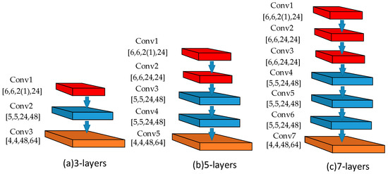
Figure 2.
Different stacked CNN network architectures for ESC. (a–c) show the CNN architectures with 3, 5, and 7 convolution layers.
We used a box plot to show the accuracy of the different network structures on different datasets under five-fold cross-validations. The results with the ESC-10 dataset (Figure 3a) show that the architecture of different stacked convolutional neural networks with log-mel feature input has some influence on their recognition accuracy. The best recognition accuracy (five-layer network) is 3.2% higher than the worst recognition accuracy (seven-layer network).
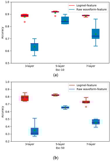
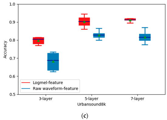
Figure 3.
Recognition accuracy of different stacked network architectures on three datasets. (a) shows the recognition accuracy on ESC-10 dataset; (b) shows the recognition accuracy on ESC-50 dataset; (c) shows the recognition accuracy on Urbansound8k.
For the raw waveform feature input, the recognition accuracy of the five-layer network model reached 85%, which is much higher than those of the other two model structures (74% for the three-layer network and 63% for the seven-layer network). On the Urbansound8k dataset (Figure 3c), we find that for the log-mel feature input, the accuracy of the five-layer network is 10.4% higher than that of the three-layer networks and matches the performance of the seven-layer network. Nevertheless, for the raw waveform feature input, the accuracy reaches the maximum (82.8%) when we adopted a five-layer network. On the ESC-50 dataset (Figure 3b), the recognition accuracy of the five-layer convolutional network is also higher than those of the other two-layer configurations. Therefore, we conclude that increasing the number of stacked network layers under the same feature does not necessarily improve recognition accuracy, and the best performance is reached by the five-layer convolutional networks. It is also found that differently from the log-mel feature input case, the stacking of more convolutional layers has a more obvious effect on the recognition accuracy with the raw waveform feature input, which makes sense due to the fact that more layers are needed to extract effective features from raw audio signals.
5.2. Filter Size Setting
In order to directly show that the strategy of using a decreasing filter size has a better performance than using a constant filter size (5,5), as in previous studies [19], and increasing filter size such as (4,4), (4,4), (5,5), (5,5), and (6,6), we conducted experiments using the ESC-50 dataset. The experimental results in Table 5 show that the best classification performance of 65.79% accuracy in RawNet and 81.09% in MelNet is achieved by using a decreasing filter size. It is indicated that the strategy of using a decreasing filter size outperforms other filter size setting strategies in our model.
Table 5.
Statistics of accuracy achieved by different filter size settings.
Furthermore, for further evaluation of whether the strategy of using a decreasing filter size outperforms other filter size setting strategies in a statistically significant way, we applied a paired sample t test. We want to test if: hypothesis (H0) is true; that is, there is no significant difference between two sets of accuracy values. The results for two paired sample t tests of accuracy values obtained by three different filter size setting strategies in RawNet and MelNet are summarized in Table 6. On average, the strategy of using a decreasing filter size has improved on the accuracy values of other strategies by 3% and 2.3% in RawNet and 1.7% and 1.8% in MelNet, respectively. The standard deviations of accuracy differences are listed in the fourth column of Table 6. The two-tailed p-values approach zero for each compared pair of RawNet and approach 0.04 in each compared pair of MelNet, which means that we should reject the H0, since the p < 0.05 in each case. It can also be seen from Table 6 that the p values indicate that the decreasing filter size has a significant effect on the accuracy.
Table 6.
Accuracy t-test results of four different filter size pairs.
5.3. Learning Rate Decay
Differently from the constant learning rate commonly used in deep neural network training schemes, we used the Adam algorithm with a learning rate decay to train the models. The dynamic learning rate formula is:
where min_learning_rate, max_learning_rate, and delay_speed are hyperparameters and is the epoch number. The max_learning_rate represents the initial learning rate. We trained both the MelNet and RawNet with three different initial rates, 0.3, 0.03, and 0.003, and found that 0.003 works best as the initial learning rate for both models. We also compared the best results with dynamic learning rates with those of constant learning rates and found that the former achieved a performance about 4% higher than that of the constant learning rate.
5.4. Batch Size Setting
For small training datasets such as ESC-10, we used the entire dataset to train and test, while for the large datasets such as ESC-50 and Urbansound8k, we used the batch mode to train and test. For training, each group of batches is constructed by randomly selecting training samples without repetition. In order to find the optimal batch size, we compared the model accuracy with different batch sizes. We evaluated the candidate batch sizes of 50, 100, 150, 200, and 250, as suggested in prior works [18,19,20], and conducted experiments on the ESC-50 dataset using the fusion model. The experimental results showed that the batch size of 200 achieved the best results and was used in all of our experiments.
5.5. Training Epoch
Due to the limited number of samples in the ESC-10 and ESC-50 datasets (even after the data augmentation), we used the early stopping approach to prevent overfitting and adopted the no-improvement-in-10-epochs strategy to identify the number of epochs. Finally, our models adopt 150, 100, and 50 training epochs, respectively, with the datasets ESC-10, ESC-50, and Urbansound8k.
5.6. When and How the DS Evidence Fusion Improves the Recognition Performance
To explore how the information fusion by DS helps to improve the performance, we created the confusion matrices of the DS-CNN, Mel-Net, and RawNet models on ESC-50 and compared the performance improvements of the DS-CNN over the other two models. Due to page limitation, we only show the confusion matrix of the DS-CNN in Figure 4 and list the comparison of recognition accuracy for all sound types before and after DS fusion in Figure 5. For the dataset Urbansound8k, all three confusion matrices are shown in Figure 6.
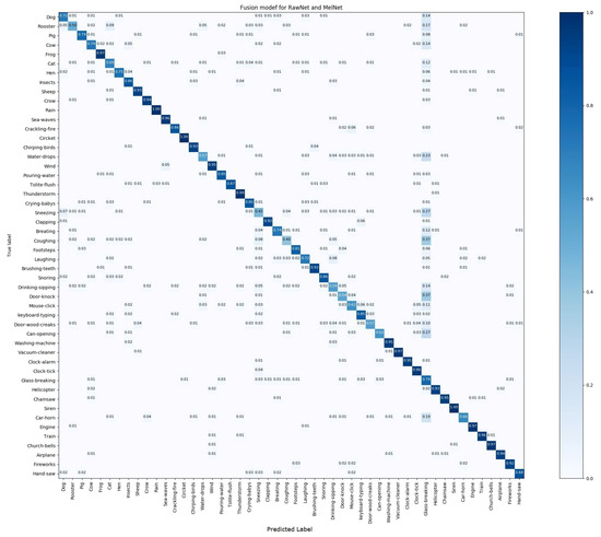
Figure 4.
Confusion matrix for the DS-CNN evaluated on the ESC-50 dataset.
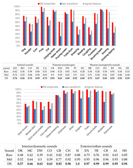
Figure 5.
Comparison of recognition accuracy for all sound types before and after DS fusion on the ESC-50 dataset.
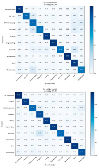
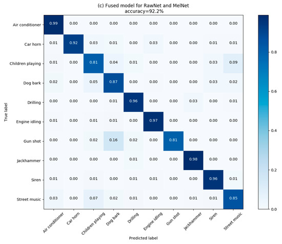
Figure 6.
Confusion matrix for RawNet (a); MelNet (b); and DS-CNN (c) models evaluated on the Urbansound8K dataset. (a) shows the each class accuracy of RawNet; (b) shows the each class accuracy of MelNet; (c) shows the each class accuracy of fusion model.
We observed that the recognition accuracy changes for each sound type, as shown in the confusion matrix before and after combination. The DS-CNN has improved the accuracy for 28 kinds of environmental sounds to varying degrees. The recognition performance over the remaining 22 kinds of environmental sounds are the same as that of the MelNet model. This implies that the combination model is capable of complementing log-mel features by learning higher level features from the raw waveform via the RawNet to help improve the performance over the 28 kinds of environmental sounds.
We further compared the accuracy of the DS-CNN with that of MelNet and RawNet on 28 environmental sound types, and present the comparison results in Figure 5. After comparison, we noticed that the recognition accuracy of the combination model obviously increases on human nonspeech and urban noises. The accuracy on seven out of 10 kinds of environmental sounds in each category has increased with the average increase rate of 6% (over urban noises) and 3.85% (over human nonspeech). Considering that these two kinds of sounds have the characteristics of continuous stability, such as for sneezing and engines, it suggests that the log-mel feature input ignores some potentially differentiating features of the continuous stability sounds. Similarly, for animal and domestic sound types, the accuracy of the DS-CNN has improved accuracy for five out of 10 different kinds of sounds, with the average increase rate of 4% and 5.8%, respectively. Moreover, these two kinds of sounds are all single sounds, which indicates that some features in the single sound can also be neglected by log-mel features. Using the DS-CNN, we can make use of features that RawNet learned from raw waveforms to complement the log-mel feature, so that the recognition accuracy can be improved via information fusion.
The experimental results on the Urbansound8k dataset also verify our conclusion. The average accuracy of the 10-fold cross-validation on the MelNet and RawNet models before model combination was 90.2% and 82.8%, respectively. After model combination, the accuracy reaches 92.2%. Figure 6a–c shows the confusion matrixes of the MelNet, RawNet, and fusion models. The diagonal elements of each matrix show the accuracy of predicting sounds of 10 classes.
At the same time, the confusion matrix in Figure 6 showed that the accuracy on six classes of environmental sounds was improved after model combination, and the six classes of sounds all share the characteristics of being single (gunshot) or steady continuous (children playing, drilling, engine idling, jackhammer, siren). This is consistent with the conclusions drawn on the ESC-50 dataset. Therefore, our DS-CNN based on DS evidence theory can make use of some sound features ignored by the log-mel feature to improve the recognition accuracy of some sound categories, and then achieve the improvement in overall accuracy with the whole dataset.
6. Conclusions
In this paper, we proposed the DS-CNN, a hybrid convolutional neural network model for environmental sound recognition. It is composed of two stacked convolutional neural networks, MelNet and RawNet, trained on log-mel feature input and raw waveform feature input, respectively. Each of these two networks are composed of five convolutional layers with batch normalization and a fully connected layer. Three public datasets, ESC-10, ESC-50, and Urbansound8k, are used to evaluate the recognition performance of the MelNet, RawNet, and DS-CNN models. The recognition accuracy of the MelNet model is 81.1%, 91%, and 90.2%, respectively, on ESC-50, ESC-10, and Urbansound8k, which is 14.6%, 4.5%, and 11.2% higher than existing CNN methods for ESC, including logmel + CNN (ESC-50, Tokozume and Harada [5]; ESC-10, Salamon and Bello [19]; Urbansound8k, Piczak [4]). Our RawNet model achieved 65.2%, 87.7%, and 85.2% accuracy on the above three datasets, which is also 1.2% and 13.52% higher than that of the state-of-the-art end-to-end methods used on the dataset (ESC-50, Tokozume, 64%; Urbansound8k, Dai, 71.68%). These results showed that our CNN models are more effective for sound recognition due to learning better high-level features from the log-mel and raw waveform inputs. Finally, we proposed the DS-CNN model based on DS evidence theory. It combines the MelNet and RawNet models to exploit the complementarity of these two CNN models. We found that DS evidence theory could substantially improve the recognition accuracy for sounds characterized with their steady continuity (such as engine noise) or single sound (gunshot) [5], but not on repeated discrete sounds, which will be a focus of future works to further improve the recognition accuracy of our DS-CNN model.
Author Contributions
Conceptualization, S.L., Y.Y. and J.H. (Jianjun Hu); Data curation, Y.Y., J.H. (Jianjun Hu) and J.H. (Jie Hu); Funding acquisition, S.L.; Investigation, Y.Y., S.L. and J.H. (Jianjun Hu); Methodology, Y.Y., J.H. (Jianjun Hu), G.L., X.Y. and J.H. (Jie Hu); Software, Y.Y.; Supervision, S.L., J.H. (Jianjun Hu); Writing—original draft, Y.Y. and J.H. (Jianjun Hu); Writing—review & editing, Y.Y. and J.H. (Jianjun Hu).
Funding
This research was funded by National Natural Science Foundation of China under Grant Nos. 91746116 and 51741101, and Science and Technology Project of Guizhou Province under Grant Nos. [2017]2308, Talents [2015]4011 and [2016]5013, Collaborative Innovation [2015]02.
Acknowledgments
We gratefully acknowledge the support of the NVIDIA Corporation with the donation of the Titan X Pascal GPU used for this research.
Conflicts of Interest
The authors declare no conflicts of interest.
Nomenclature
| DO | Dog |
| RO | Rooster |
| CO | Cow |
| FR | Frog |
| CA | Cat |
| CB | Chirping-birds |
| WD | Water-drops |
| PW | Pouring-water |
| TF | Toilet-flush |
| SN | Sneezing |
| BR | Breathing |
| CO | Coughing |
| FO | Footsteps |
| BT | Brushing-teeth |
| SN | Snoring |
| DS | Drinking-sipping |
| DK | Door Knock |
| MC | Mouse-click |
| DW | Door-wood-creaks |
| CO | Can-opening |
| GB | Glass-breaking |
| CH | Chainsaw |
| SI | Siren |
| EN | Engine |
| TR | Train |
| CB | Church-bells |
| AI | Airplane |
| HS | Hand-saw |
References
- Piczak, K.J. ESC: Dataset for Environmental Sound Classification. In Proceedings of the ACM International Conference on Multimedia, Brisbane, Australia, 26–30 October 2015. [Google Scholar]
- Łopatka, K.; Zwan, P.; Czyżewski, A. Dangerous Sound Event Recognition Using Support Vector Machine Classifiers; Springer: Berlin/Heidelberg, Germany, 2010; pp. 49–57. [Google Scholar]
- Mydlarz, C.; Salamon, J.; Bello, J.P. The implementation of low-cost urban acoustic monitoring devices. Appl. Acoust. 2016, 117, 207–218. [Google Scholar] [CrossRef]
- Piczak, K.J. Environmental sound classification with convolutional neural networks. In Proceedings of the IEEE International Workshop on Machine Learning for Signal Processing, Boston, MA, USA, 17–20 September 2015; pp. 1–6. [Google Scholar]
- Tokozume, Y.; Harada, T. Learning environmental sounds with end-to-end convolutional neural network. In Proceedings of the IEEE International Conference on Acoustics, Speech and Signal Processing, New Orleans, LA, USA, 5–9 March 2017. [Google Scholar]
- Han, Y.; Lee, K. Acoustic scene classification using convolutional neural network and multiple-width frequency-delta data augmentation. arXiv, 2016; arXiv:1607.02383. [Google Scholar]
- Cotton, C.V.; Ellis, D.P.W. Spectral vs. spectro-temporal features for acoustic event detection. In Proceedings of the Applications of Signal Processing to Audio and Acoustics, New Paltz, NY, USA, 16–19 October 2011. [Google Scholar]
- Geiger, J.T.; Schuller, B.; Rigoll, G. Large-scale audio feature extraction and SVM for acoustic scene classification. In Proceedings of the Applications of Signal Processing to Audio and Acoustics, New Paltz, NY, USA, 20–23 October 2013. [Google Scholar]
- Ntalampiras, S.; Potamitis, I.; Fakotakis, N. Automatic recognition of urban environmental sounds events. In Proceedings of the IAPR Workshop on Cognitive Information Processing Cip, Santorini, Greece, 9–10 June 2008. [Google Scholar]
- Barchiesi, D.; Giannoulis, D.; Dan, S.; Plumbley, M.D. Acoustic Scene Classification: Classifying environments from the sounds they produce. IEEE Signal Process. Mag. 2015, 32, 16–34. [Google Scholar] [CrossRef]
- Chachada, S.; Kuo, C.C.J. Environmental sound recognition: A survey. In Proceedings of the Signal and Information Processing Association Summit and Conference, Hollywood, CA, USA, 3–6 December 2012. [Google Scholar]
- Theodorou, T.; Mporas, I.; Fakotakis, N. Automatic Sound Recognition of Urban Environment Events; Springer International Publishing: Berlin/Heidelberg, Germany, 2015; pp. 129–136. [Google Scholar]
- Su, F.; Yang, L.; Lu, T.; Wang, G. Environmental sound classification for scene recognition using local discriminant bases and HMM. In Proceedings of the International Conference on Multimedea, Scottsdale, AZ, USA, 28 November–1 December 2011. [Google Scholar]
- Gencoglu, O.; Virtanen, T.; Huttunen, H. Recognition of acoustic events using deep neural networks. In Proceedings of the Signal Processing Conference, Lisbon, Portugal, 1–5 September 2014. [Google Scholar]
- Mcloughlin, I.; Zhang, H.; Xie, Z.; Song, Y.; Xiao, W. Robust Sound Event Classification Using Deep Neural Networks. IEEE/ACM Trans. Audio Speech Lang. Process. 2017, 23, 540–552. [Google Scholar] [CrossRef]
- Kons, Z.; Toledo-Ronen, O. Audio event classification using deep neural networks. In Proceedings of the INTERSPEECH 2013, Lyon, France, 25–29 August 2013. [Google Scholar]
- Sivaprakasam, T.; Dhanalakshmi, P. A robust environmental sound event recognition using spectral features. Int. J. Appl. Eng. Res. 2014, 9, 5157–5162. [Google Scholar]
- Huzaifah, M. Comparison of Time-Frequency Representations for Environmental Sound Classification using Convolutional Neural Networks. arXiv, 2017; arXiv:1706.07156. [Google Scholar]
- Salamon, J.; Bello, J. Deep Convolutional Neural Networks and Data Augmentation for Environmental Sound Classification. IEEE Signal Process. Lett. 2017, 24, 279–283. [Google Scholar] [CrossRef]
- Hoshen, Y.; Weiss, R.J.; Wilson, K.W. Speech acoustic modeling from raw multichannel waveforms. In Proceedings of the IEEE International Conference on Acoustics, Speech and Signal Processing, Brisbane, Australia, 19–24 April 2015. [Google Scholar]
- Zazo, R.; Sainath, T.N.; Simko, G.; Parada, C. Feature Learning with Raw-Waveform CLDNNs for Voice Activity Detection. In Proceedings of the INTERSPEECH 2016, San Francisco, CA, USA, 8–12 September 2016. [Google Scholar]
- Dai, W.; Dai, C.; Qu, S.; Li, J.; Das, S. Very deep convolutional neural networks for raw waveforms. In Proceedings of the IEEE International Conference on Acoustics, Speech and Signal Processing, New Orleans, LA, USA, 5–9 March 2017. [Google Scholar]
- Aytar, Y.; Vondrick, C.; Torralba, A. SoundNet: Learning Sound Representations from Unlabeled Video. arXiv, 2016; arXiv:1610.09001. [Google Scholar]
- Hégarat-Mascle, S.L.; Bloch, I.; Vidal-Madjar, D. Application of Dempster-Shafer evidence theory to unsupervised classification in multisource remote sensing. Geosci. Remote Sens. 1997, 35, 1018–1031. [Google Scholar] [CrossRef]
- Li, Y.-B.; Wang, N.; Zhou, C. Based on D-S evidence theory of information fusion improved method. In Proceedings of the International Conference on Computer Application and System Modeling, Taiyuan, China, 22–24 October 2010. [Google Scholar]
- Yao, X.; Li, S.; Hu, J. Improving Rolling Bearing Fault Diagnosis by DS Evidence Theory Based Fusion Model. J. Sens. 2017, 2017, 6737295. [Google Scholar] [CrossRef]
- Dou, Z.; Xu, X.; Lin, Y.; Zhou, R. Application of D-S Evidence Fusion Method in the Fault Detection of Temperature Sensor. Math. Probl. Eng. 2014, 2014, 395057. [Google Scholar] [CrossRef]
- Hui, K.H.; Meng, H.L.; Leong, M.S.; Al-Obaidi, S.M. Dempster-Shafer evidence theory for multi-bearing faults diagnosis. Eng. Appl. Artif. Intell. 2017, 57, 160–170. [Google Scholar] [CrossRef]
- Salamon, J.; Jacoby, C.; Bello, J.P. A Dataset and Taxonomy for Urban Sound Research. In Proceedings of the ACM International Conference on Multimedia, Orlando, FL, USA, 3–7 November 2014. [Google Scholar]
- Davis, S.B.; Mermelstein, P. Comparison of Parametric Representations for Monosyllabic Word Recognition in Continuously Spoken Sentences. Read. Speech Recognit. 1980, 28, 65–74. [Google Scholar] [CrossRef]
- Abdel-Hamid, O.; Mohamed, A.R.; Jiang, H.; Deng, L.; Penn, G.; Yu, D. Convolutional Neural Networks for Speech Recognition. IEEE/ACM Trans. Audio Speech Lang. Process. 2014, 22, 1533–1545. [Google Scholar] [CrossRef]
- Jaitly, N.; Hinton, G. Learning a better representation of speech soundwaves using restricted boltzmann machines. In Proceedings of the IEEE International Conference on Acoustics, Speech and Signal Processing, Prague, Czech Republic, 22–27 May 2011. [Google Scholar]
- Palaz, D.; Collobert, R.; Doss, M.M. Estimating Phoneme Class Conditional Probabilities from Raw Speech Signal using Convolutional Neural Networks. arXiv, 2013; arXiv:1304.1018. [Google Scholar]
- Lee, J.; Park, J.; Kim, K.L.; Nam, J. Sample-level Deep Convolutional Neural Networks for Music Auto-tagging Using Raw Waveforms. arXiv, 2017; arXiv:1703.01789. [Google Scholar]
- Dinkel, H.; Chen, N.; Qian, Y.; Yu, K. End-to-end spoofing detection with raw waveform CLDNNS. In Proceedings of the IEEE International Conference on Acoustics, Speech and Signal Processing, New Orleans, LA, USA, 5–9 March 2017. [Google Scholar]
- Muckenhirn, H.; Magimai-Doss, M.; Marcel, S. End-to-End convolutional neural network-based voice presentation attack detection. In Proceedings of the IEEE International Joint Conference on Biometrics, Denver, CO, USA, 1–4 October 2017. [Google Scholar]
- Dempster, A.P. Upper and Lower Probabilities Induced by a Multivalued Mapping. Ann. Math. Stat. 1967, 38, 325–339. [Google Scholar] [CrossRef]
- Lndley, D.V. A mathematical theory of evidence. Technometrics 1977, 20, 106. [Google Scholar] [CrossRef]
- Simonyan, K.; Zisserman, A. Very Deep Convolutional Networks for Large-Scale Image Recognition. arXiv, 2014; arXiv:1409.1556. [Google Scholar]
© 2018 by the authors. Licensee MDPI, Basel, Switzerland. This article is an open access article distributed under the terms and conditions of the Creative Commons Attribution (CC BY) license (http://creativecommons.org/licenses/by/4.0/).