Aerodynamic Performance of Wind Turbine Airfoil DU 91-W2-250 under Dynamic Stall

Abstract

Airfoils are subjected to the ‘dynamic stall’ phenomenon in significant pitch oscillations during the actual operation process of wind turbines. Dynamic stall will result in aerodynamic fatigue loads and further cause a discrepancy in the aerodynamic performance between design and operation. In this paper, a typical wind turbine airfoil, DU 91-W2-250, is examined numerically using the transition shear stress transport (SST) model under a Reynolds number of $3\times {10}^5$. The influence of a reduced frequency on the unsteady dynamic performance of the airfoil model is examined by analyzing aerodynamic coefficients, pressure contours and separation point positions. It is concluded that an increasingly-reduced frequency leads to lower aerodynamic efficiency during the upstroke process of pitching motions. The results show the movement of the separation point and the variation of flow structures in a hysteresis loop. Additionally, the spectrum of pressure signals on the suction surface is analyzed, exploring the level of dependence of pressure fluctuation on the shedding vortex and oscillation process. It provides a theoretical basis for the understanding of the dynamic stall of the wind turbine airfoil.

1. Introduction

Wind turbines operate in diverse environments under complex control strategies, suffering unsteady loads including aerodynamic forces. An important source of these forces comes from the blades when the relative velocity with respect to blade sections varies in magnitude and direction. Generally, the airfoils on the blades are considered as operating in dynamic stall [1]. The unsteady factors that cause dynamic stall are, e.g., wind shear and yaw, and the angles of attack of airfoils periodically vary with the rotation of blades [2,3,4]. Then, the stall characteristics are dynamically dependent on the operating route of airfoils with dramatically different lift and drag forces from those in static operations. The main disadvantage of dynamic stall for the safety of blades is that it causes fatigue loads and a deviation between design and actual running conditions. With the trend of the large-scale development of wind turbines, dynamic stall will have increasingly greater influence on the unsteady aerodynamic characteristics of wind turbine blades.

Dynamic stall has been one of the major interesting research subjects and has been studied over the latest few decades. The dynamic stall phenomenon was first observed in the 1930s [5]. It was first systematically studied in the aerospace field and was studied in a wider field later, such as for maneuverable jets wings, gas turbines and wind turbines [6]. Previous studies primarily concentrating on dynamic stall consist of experimental and numerical simulation. Experiments are important because experimental data provide a verification basis for the numerical simulation. However, due to the limitation of experimental conditions and other reasons, it is necessary to employ numerical simulation to grasp a broader and more general conclusion. With the gradual maturity of the theory, there are many analytical models to predict the effects of dynamic stall and analyze the load of power machines nowadays; such as the Boeing–Vertol model [7], the ONERA model [8], the Beddoes–Leishman (B–L) semi-empirical model [9], etc. The B-L model has been adopted most widely to analyze dynamic stall. It has been modified and improved with the increasing attention on unsteady aerodynamics [10,11,12,13]. The modified model shows better agreement than the original one. Although the semi-empirical models have the advantage of using less computational resources, they depend on the accuracy of the empirical factors greatly, and it is not possible to obtain detailed and accurate flow field information. With the development of computer technology, the computational fluid dynamics (CFD) method is used to study dynamic stall for the purpose of obtaining detailed information of dynamic stall. Some researchers have been dedicated to finding more accurate turbulence models. For example, Martinat et al. [14] used three turbulence models to investigate the dynamic stall of a NACA 0012 airfoil, and the unsteady Reynolds-averaged Navier–Stokes (URANS) $k-\epsilon$ Chien model provided the best results. Wang et al. [15] compared the renormalization-group (RNG) $k-\epsilon$ model and transition shear stress transport (SST) $k-\omega$ model used to simulate dynamic stall of an oscillating NACA 0012 airfoil at a relatively low Reynolds number. It was found that the SST $k-\omega$-based detached eddy simulation (DES) approach was superior. Some other researchers have focused on how typical factors affecting dynamic stall. These factors include the Reynolds number, mean angle of pitch oscillation, amplitude of pitch oscillation, reduced frequency, the position of pitch axis, turbulence intensity, etc. For instance, Akbari et al. [16] studied the effects of reduced frequency, mean angle of attack, pitch axis location and Reynolds number on the dynamic stall of a NACA 0012. It was shown that the reduced frequency was the most influential parameter on dynamic stall. Gharali et al. [17] investigated the effects of the oscillations of the free-stream velocity on pitch oscillation by the SST $k-\omega$ model; Kim et al. [18] studied the effects of free-stream turbulence on the aerodynamic characteristics of pitching airfoils by large eddy simulations. Gandhi et al. [19] investigated the influence of reduced frequency on the dynamic stall characteristics of a NACA 0012 airfoil pitching in a turbulent wake with direct numerical simulations. In addition, McCroskey and his partners made two efforts for decades to investigate the details of the dynamic stall phenomena [20,21,22]. The above results are extensive and continuous. However, the problem is that most of the research objects are wings or symmetrical airfoils. The literature lacks observations of specific asymmetric and blunt tail edge wind turbine airfoils, such as Delft University of Technology (DU) series airfoils. On the other hand, the flow field contour is a general method to explain the phenomenon of dynamic stall used by many previous researchers. It is summarized that a typical dynamic stall process consists of four major stages: attached flow at low angles of attack, the development of the leading edge vortex (LEV), the shedding of the LEV from the suction surface and reattachment of the flow to the suction surface [23]. However, there is a little attention given to the relationship between the frequency of shedding vortices and the frequency of airfoil pitching motion. The interpretation of the “delay” is always analyzed by the lift and drag coefficients or the qualitative expression of the flow field contours. The quantitative expression of the separation of the airfoil boundary layer is not obviously given.

In order to avoid flow separation and reduce the dynamic stall effects, various devices have been proposed for flow control. Depending on the operating principle, they can be classified as active or passive [24]. Passive control includes vortex generators, microtabs, serrated trailing edges, and so on. Active control includes trailing-edge flaps, synthetic jets, and so on. Johnson et al. [25] overviewed 15 different devices for wind turbine control. Lei Zhang et al. [26,27] made long-term efforts to investigate the effects of vortex generators. Some other researchers focused on microtabs [28,29] and obtained some good results. T.K. Barlas et al. [30] and Unai Fernandez-Gamiz et al. [31] reviewed some devices and discussed their effects. The flow control devices have good effects on avoiding flow separation, but the blades have a higher cost for their production. Based on the above, cases with different reduced frequencies (the most important influential factor) are compared regarding the aerodynamic forces and lift-to-drag ratio. In addition, the delay effect of dynamic stall is deeply analyzed from the perspective of two aspects: the pressure field and spectrum analysis.

2. Method

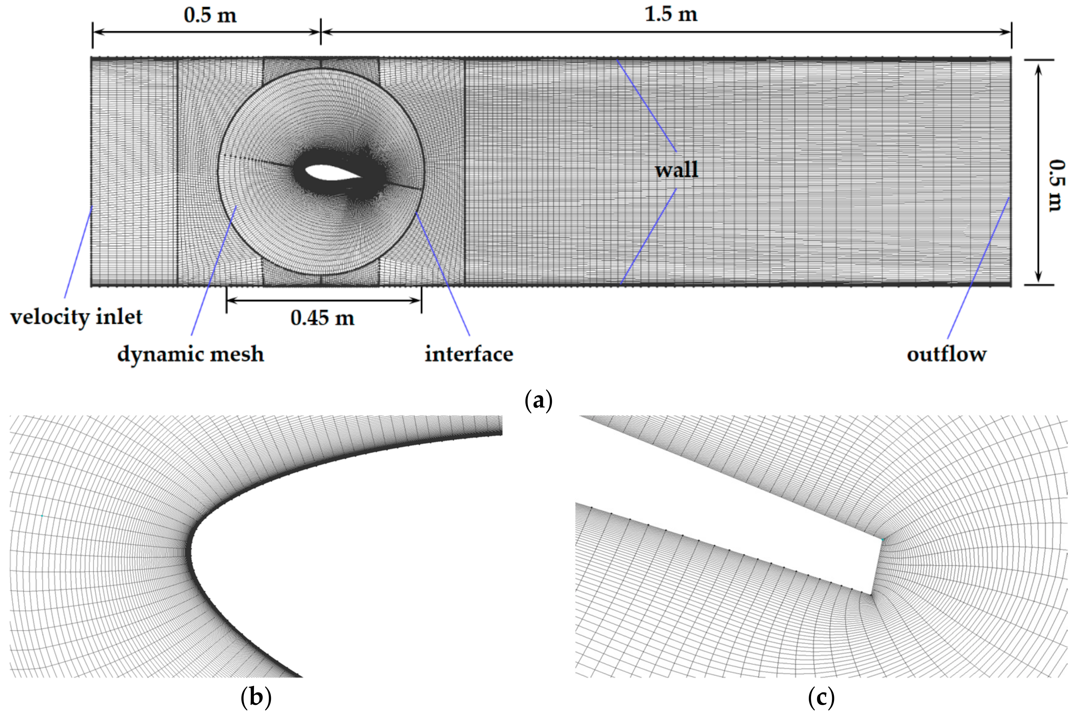
2.1. Numerical Method

The airfoil DU 91-W2-250 was developed by TU Delft, which has a relative thickness of 25% with a trailing edge gap of 0.65% chord [32]. The present study is based on a 2D simulation with ceiling and bottom boundary similarity in a wind tunnel. With this kind of set, the numerical method is easily validated by the authors’ previous measurements [33]. In order to simulate the dynamic stall phenomenon, a rotational zone whose radius is three-times that of the model chord is placed at the pitching center, as shown in Figure 1. The rotational zone and airfoil model oscillate like a rigid body, and the movement is defined with a user-defined function (UDF) in ANSYS Fluent [22]. The rest of grid is connected to the rotational grid by interfaces. The block interfaces between the dynamic and static zones are non-conformal because, as the airfoil moves, the O-grid attached to the airfoil rotates rigidly (as a solid body) together with the airfoil.

The Reynolds number is $3\times {10}^5$, which confirmed the turbulence that appeared in the previous study. Flows under such a relatively low Reynolds number are highly non-linear [34]. Therefore, turbulence should be considered in the simulation. There are three main turbulence simulation methods, i.e., direct numerical simulation (DNS), Reynolds-averaged Navier–Stokes (RANS) and large eddy simulation (LES). A turbulence model should present a satisfactory representation of an important phenomenon while introducing the least amount of complexity [35]. In the present study, considering numerical simulation cost and acceptable accuracy, the unsteady Reynolds-averaged Navier–Stokes (URANS) method is seem to be the most suitable one to simulate the dynamic stall phenomenon [15]. Consequently, in the CFD software ANSYS Fluent, the transition SST k − ω model, which is capable of capturing the transition process, was chosen. Some researchers have also discussed that the accuracy of this model is satisfactory [15,17,36,37,38,39,40].

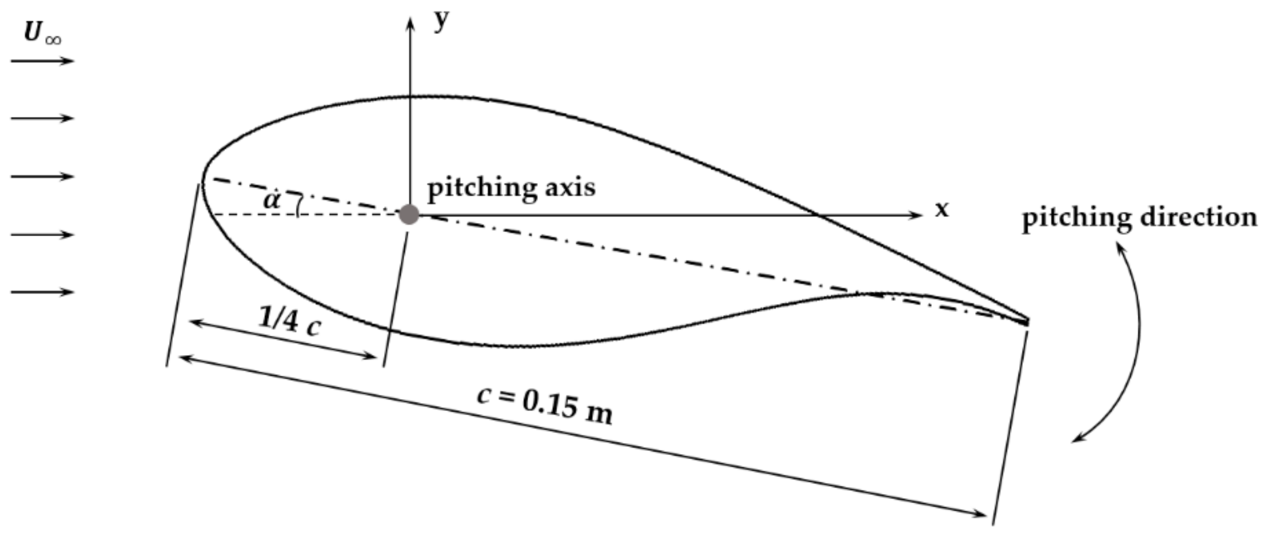
2.2. Oscillation of the Airfoil

The movement of the airfoil model is described as Equation (1) in a sinusoidal mode, as shown in Figure 2.

$${\alpha }_t={\alpha }_0+{\alpha }_{amp}\sin \left(\omega t\right),$$

(1)

where,

• ${\alpha }_t$ is the angle of attack at flow time t,
• ${\alpha }_0$ is the mean angle of attack,
• ${\alpha }_{amp}$ is the pitch oscillation amplitude,
• $\omega$ is the oscillation angular frequency.

The angular frequency $\omega$ is related to the reduced frequency k, which is an important parameter used to describe the ‘degree of unsteadiness’, as defined by Equation (2).

$$k= \frac{\omega c}{2U_{\infty }}$$

(2)

where $U_{\infty }$ is the free-stream velocity and c is the chord length of the airfoil. It can be obtained from dimensionless Navier-Stokes (N-S) equations. J. G. Leishman has the empirical view that when 0 $\le k\le 0.5$, the flow can be considered as quasi-steady flow, which means for some cases that the unsteady effects may be neglected completely [1]. Therefore, k = 0.026, 0.502 and 0.106 are set to be computed to find out whether the previous empirical view applies to the pitching motion of the DU 91-W2-250 airfoil. They correspond to the oscillating period T = 0.6 s, 0.3 s and 0.15 s, respectively.

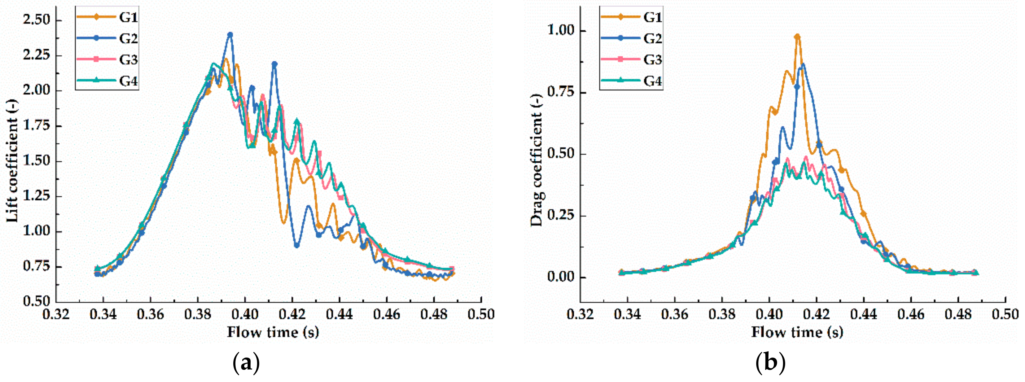
2.3. Grid Sensitivity

The independence of the solution from the grid is examined by different grid densities in

Table 1. Cases for grid sensitivity examination.

Grid	Suction Surface	Pressure Surface	Trailing Edge	Total Grids
G1	50 1	50	11	25,753
G2	100	100	11	45,387
G3	150	150	11	67,238
G4	200	200	11	89,070

¹ The number of cells on the indicated surfaces.

. Only the circumferential grid densities are changed, but the radial grid densities are the same. The growth rate of grid is set as 1.05, and the maximum grid is 0.3c. It is important that the mesh near the wall be properly sized to ensure accurate simulation and no wall functions are used [41]. The height of the first mesh cell off the wall is ${10}^{-5}$ m, so that the non-dimensional wall-distance $y^{+}$ [42] is less than 1.0 at a Reynolds number of $3\times {10}^5$. It is computed by using flat-plate boundary layer theory [43]. The lift and drag coefficients during the 4th cycle of pitching motion are shown in Figure 3. The comparison shows that the numerical results for grid cases G3 and G4 do not differ considerably from other grid densities. In order to observe more detailed characteristics on the suction surface of the airfoil, the grid nodes on the suction side are increased to 200 and keep the same set of grids as G3 on the pressure side of the airfoil.

2.4. Time Step and Periodic Repeatability

To specify the optimum time step in the unsteady simulations, a series case with different time steps was simulated. A characteristic time $T_c$ defined by Equation (3) is employed as base of the time step:

$$T_c= \frac{c}{U_{\infty }}$$

(3)

It has the same significance as the Courant, Friedrichs and Levy criterion (CFL) number in numerical simulations. The time steps of 0.1${\mathrm{T}}_c$, 0.05${\mathrm{T}}_c$, 0.025${\mathrm{T}}_c$, 0.0125${\mathrm{T}}_c$ and 0.00625${\mathrm{T}}_c$ (denoted as dt1 to dt5, respectively) are used to examine the time step sensitivity.

As shown in Figure 4, when the time step dt4 = $6.25\times {10}^{-5}$ s, the time cost and accuracy are acceptable for the present study. This is consistent with dynamic stall cases applied by other researchers [17,38].

Periodic repeatability is also examined, as shown in Figure 5. It shows that values tend to be well reproducible from the third cycle. That is why the other cases are computed only for 4 periods.

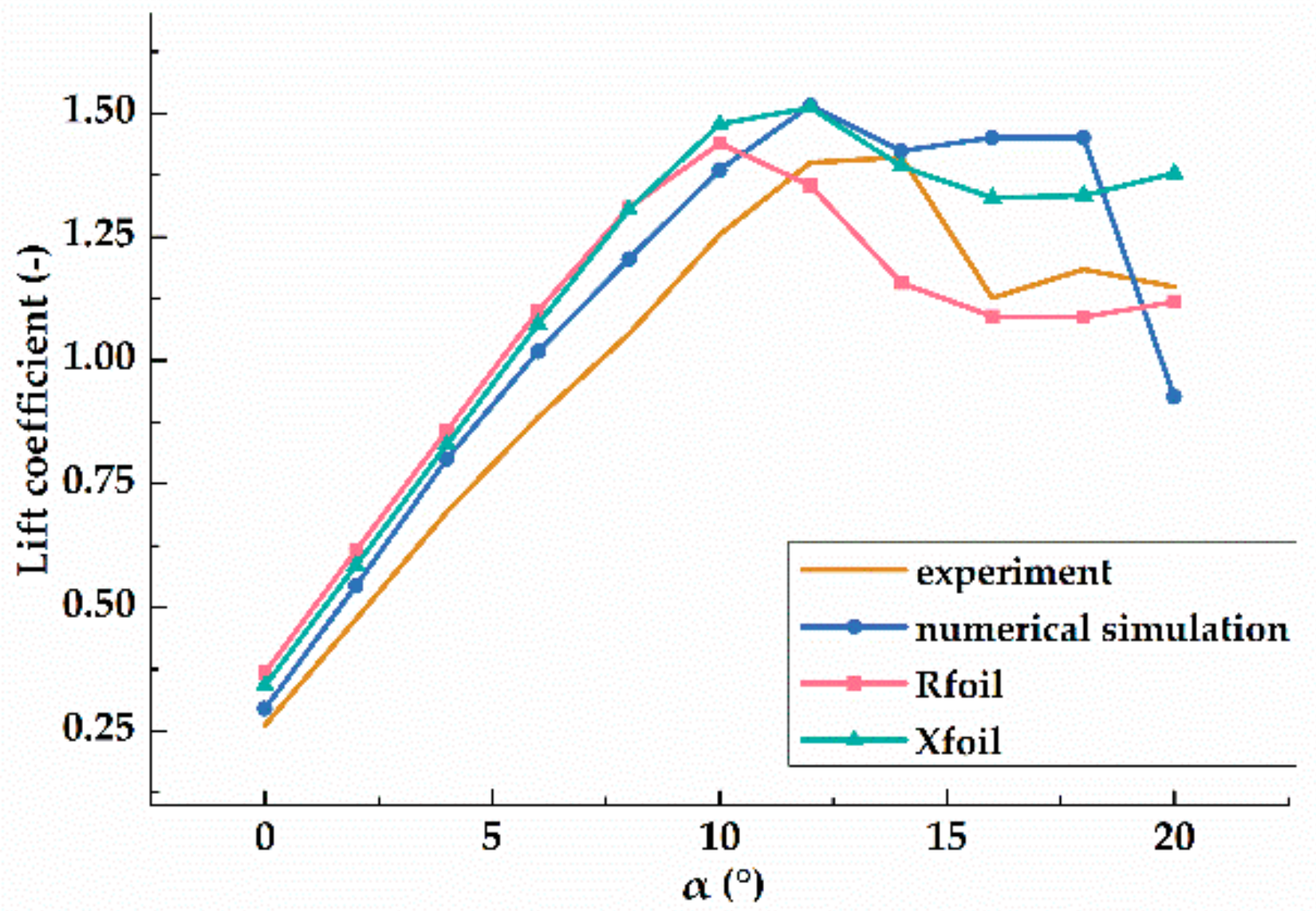
2.5. Comparison of the Static Result with Experiment and Vortex Panel Method

Due to the lack of experimental data for the dynamic stall of the DU 91-W2-250 airfoil at present, the static experimental data, which have been obtained from Jingyan Bai et al. [33], are used to examine the accuracy of the numerical method. The data computed by the software Xfoil and Rfoil, which are currently widely accepted, are also compared to each other, as shown in Figure 6.

Generally, Xfoil and Rfoil predict acceptable lift and drag coefficients for thin airfoils in attached flow. It is shown that the numerical simulation is more consistent with the data obtained by Xfoil. Because of the constraints of the experimental equipment and conditions in 2014, a large discrepancy appears between the experimental and CFD results. The accuracy of the zero angle of attack and the stiffness of the support structure may be the main factors, which usually cause the shift of the lift curve along the angle-axis and the variation of the slope of the linear section on the lift curve, respectively. Moreover, CFD greatly overestimates the lift coefficient at 18 and 20 with respect to that of Xfoil, Rfoil and the experiment. This is because the airfoil goes into a deep stall and the flow becomes fully separated at high angles of attack. Raffel et al. [44] showed that the 3D effects of separation flows should be more significant than those without separations at smaller angles of attack. Therefore, in the following analysis, static data calculated by Xfoil are considered as baseline data in the static condition.

3. Results and Discussions

In this part, the results of the cases defined in Section 2.2 are analyzed. The performance of airfoil DU 91-W2-250 under dynamic stall is illustrated with respect to three aspects, i.e.: (a) the influence of reduced frequency; (b) flow structures and separation points; and (c) spectrum characteristics.

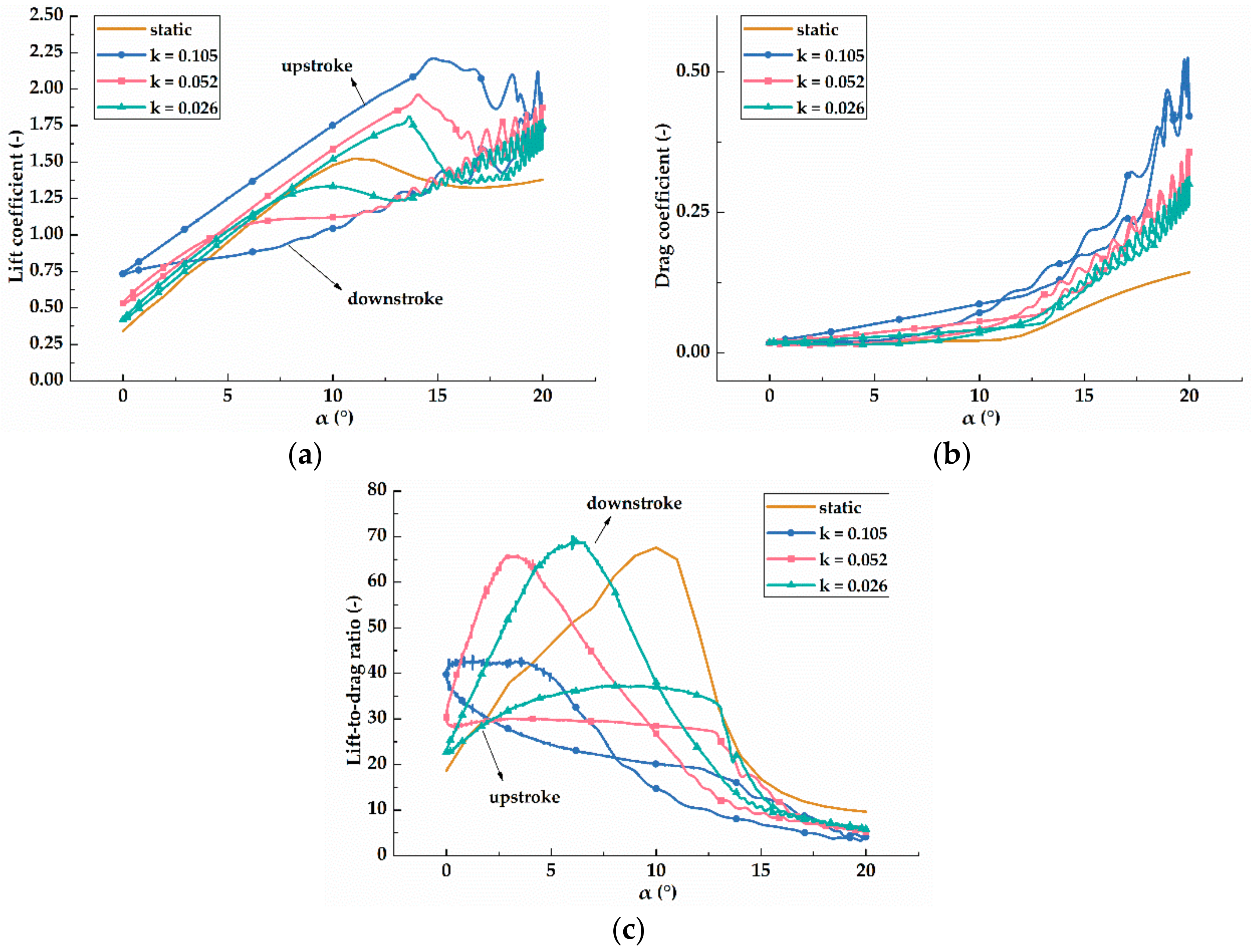
3.1. Effects of Reduced Frequency on Aerodynamic Coefficients

Three cases when k = 0.026, 0.502 and 0.106 were simulated, and the results are shown in Figure 7. The dynamic characteristics of the airfoil undergoing pitch oscillation were strongly dependent on the reduced frequency. The hysteresis loop increased with the increasingly-reduced frequency. In a loop, as can be seen, the maximum lift coefficient in upstroke and the corresponding angle of attack were much higher than those in the static condition. Previous researchers have observed this phenomenon already as mentioned in Section 1. Contrarily, the lift coefficient in downstroke was smaller than that in upstroke and sometimes even smaller than that in the static condition. On the lift curves, the intersection point in a loop was named the “reunion point” by the authors. An increase in the reduced frequency made the angle of reunion point smaller. This also means that the effect of delay was more significant when the frequency reduction was greater. On the other hand, the increasingly-reduced frequency would cause the increase of the drag coefficient. This effect is clearly revealed in the lift-drag-ratio curve in Figure 7c.

The lift-to-drag ratio is an important parameter that indicates the aerodynamic efficiency of the airfoils. The aerodynamic performance of the airfoils is better with a larger lift-to-drag ratio. The angle of attack corresponding to the maximum lift-to-drag ratio is called a favorable angle of attack. In general, from the minimum angle to the favorable angle of attack, lift increases fast, but drag increases slowly. Therefore, the lift-to-drag ratio increases. Then, from the favorable angle to a critical stall angle of attack, the increase of lift is slow, and the drag increases rapidly. This makes the lift-to-drag ratio relatively small. After the critical stall angle of attack, the lift-to-drag ratio sharply decreases with the sharply increasing pressure drag. The lift-to-drag ratio of the airfoil during a complete hysteresis loop was quite different with a regular pattern. The peak of the lift-to-drag ratio curve in upstroke decreased and even disappeared with the increasingly-reduced frequency because of the faster increase of the drag coefficient. This effect was amplified in the lift-to-drag ratio and showed the tremendous difference between static and dynamic stall. Instead, the lift-to-drag ratio in the downstroke process showed a different form. Its shape was closer to the static form, which also had a peak. The angle of attack corresponding to the peak was smaller with increasingly-reduced frequency. This also shows the degree of the delay effect. Therefore, the aerodynamic efficiency was lower in dynamic stall process though the lift in upstroke was higher than that in the static condition.

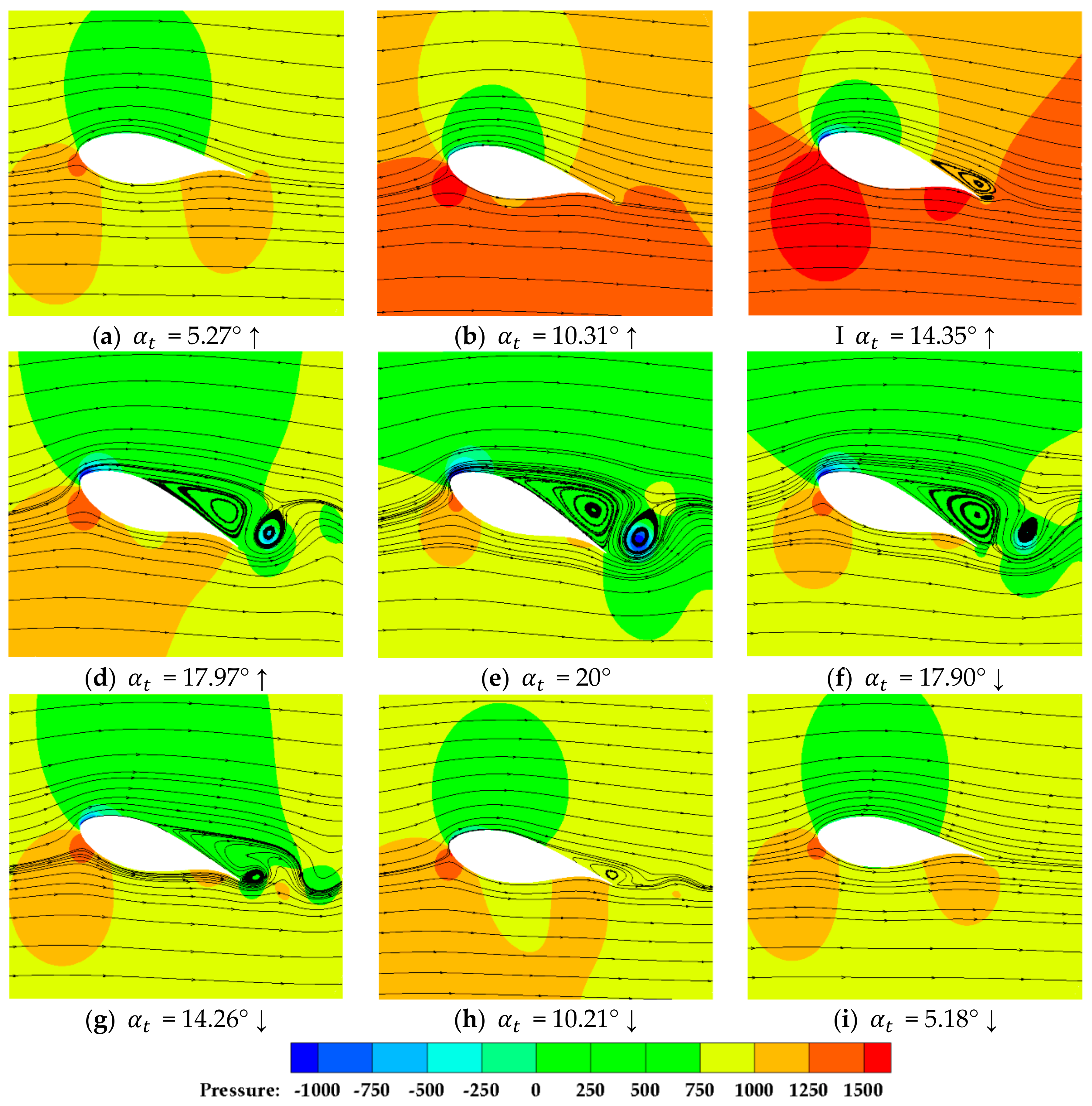
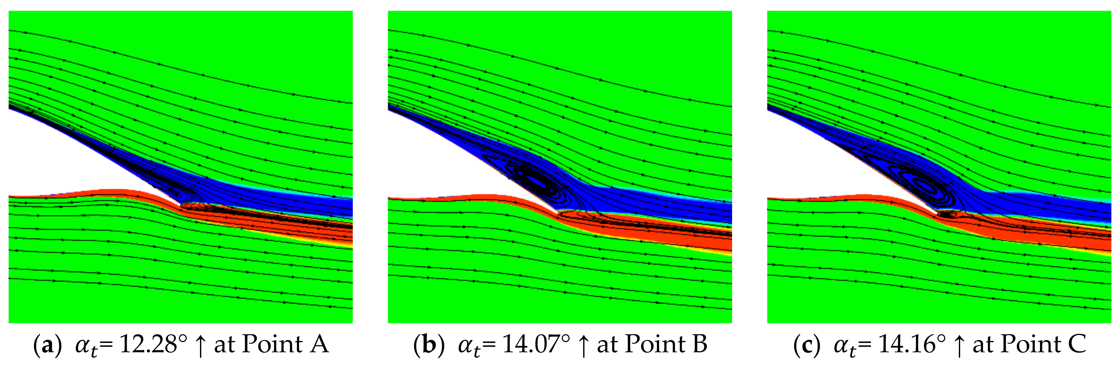
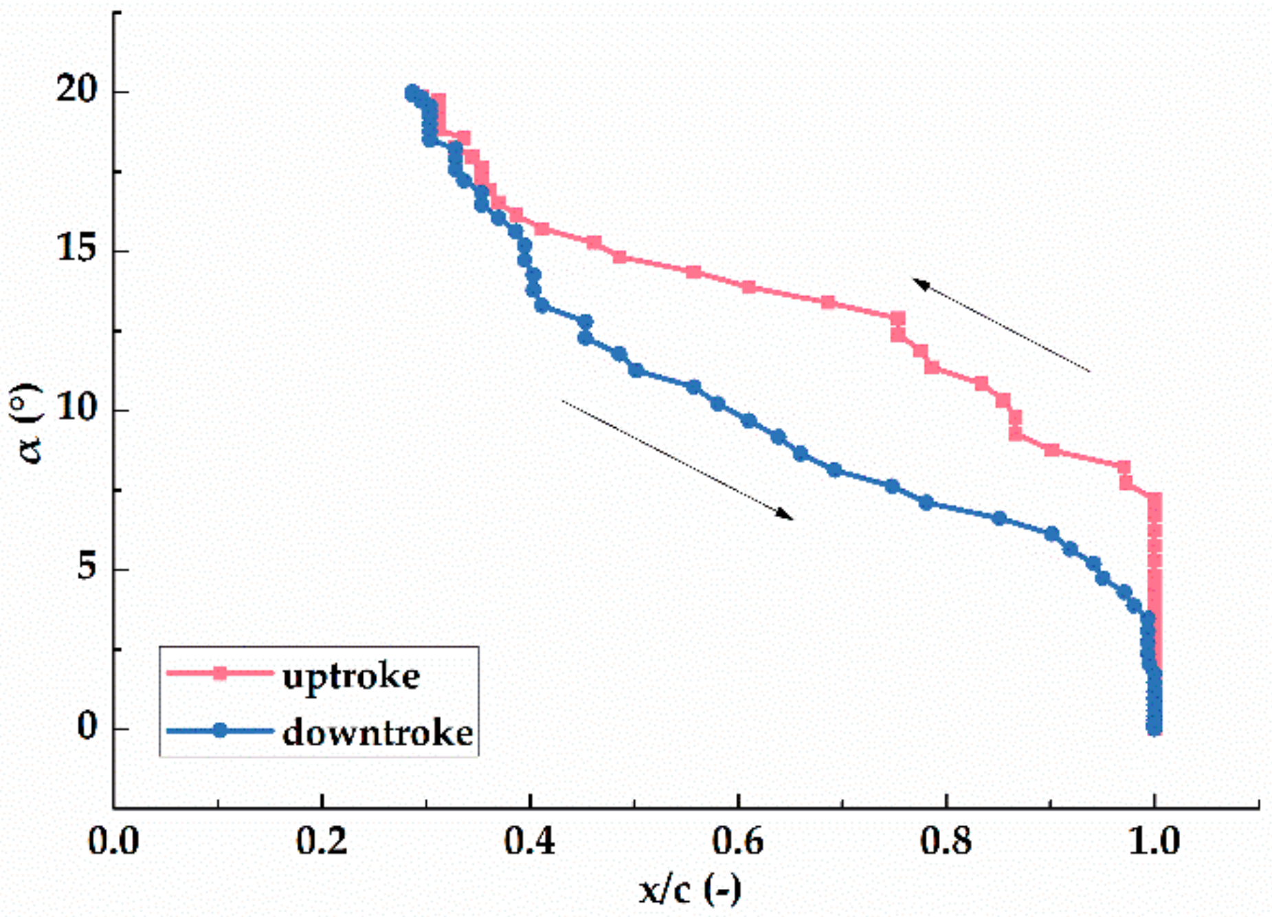
3.2. Flow Development and Separation Points on the Suction Surface of the Airfoil

The reason for the variation of forces and lift-to-drag ratio can be found in flow field contours. One case was selected to investigate the characteristics as an example. The pressure fields and corresponding streamlines at different angles of attack through a full pitching cycle in the case with k = 0.052, ${\alpha }_0$ = 10°, ${\alpha }_{amp}$ = 10° are demonstrated in Figure 8. It was observed that the development trend of flow field structures of the DU 91-W2-250 was qualitatively in good agreement with the conclusions of other papers with different shapes of airfoils [15,45,46]. The flow was fully attached to the airfoil from the angles of attack ${\alpha }_t$ = 0°~10.31°. The hysteresis of stall angles of attack in lift curves, which is the most obvious feature of dynamic stall, is observed clearly here. The lift dropped suddenly at about 14$°$ in the hysteresis loop, while the static stall angle was 12° in the experiment. It was manifested as reversed flow generated near the trailing edge, as shown in Figure 8c. The reverse flow was due to the adverse pressure gradient caused by the rapid movement of the airfoil surface. As the angle of attack increased, the clockwise-rotating vortex on the suction surface moved forward to the leading edge, and the strength of the recirculation increased. There was a small counterclockwise-rotating vortex behind the trailing edge vortex in Figure 8c, implying that the vortex near the trailing edge started to move downstream slowly. This would lead to a decrease in the lift coefficient compared with the lift coefficient curves in Figure 7a. The effects of vortices rotating in two opposite directions on the lift coefficient are shown in Figure 9 in more detail. At Point A in Figure 9a, the clockwise-rotating vortex appeared. With the growth of the vortex, the lift coefficient was still increasing. The growing vortex increased the slope of the lift curves until the maximum value of $C_l$ when the angle of attack was 14.07$°$ at Point B; see Figure 9b. The reason that $C_l$ decreased was the generation of the counterclockwise-rotating vortex, as shown in Figure 9c. $C_l$ decreased with the growth of the counterclockwise-rotating vortex until the counterclockwise-rotating vortex traveled into the wake and the clockwise-rotating vortex appeared again; see Figure 9e. This process would repeat until the trend of the lift coefficient curve became flat when ${\alpha }_t$ = 10.31$°$ in the downstroke process. The counterclockwise-rotating vortex did not appear from this moment. In other words, the growth and shedding of vortices in opposite directions led to the fluctuations of the lift coefficient curve. The lift coefficient $C_l$ increased with the growth of the vortex, and it decreased with the shedding of the vortex. What needs to be noted here is that the range of the angles of attack in this case was from 0$°$–20$°$, so the airfoil did not experience a deep stall. Vortices on the suction surface of airfoil did not develop to reach the leading edge, but only reached 30% of the chord from the leading edge. Therefore, in this case with k = 0.052, ${\alpha }_0$ = 10°, ${\alpha }_{amp}$ = 10°, the LEV observed in other papers [15] did not appear, but it appeared when k = 0.052, ${\alpha }_0$ = 15°, ${\alpha }_{amp}$ = 10°. After the maximum angle of 20°, the airfoil was performing the downstroke motion. It is known that the lift coefficient of the downstroke process was much smaller than the upstroke process from Section 3.1. This is because the vortex still existed near the trailing edge and the pressure of pressure surface was lower at the same angle of attack by comparing Figure 8b,h and Figure 8c,g. As the airfoil attack angle became smaller, vortices eventually moved into the wake. The last vortex left the trailing edge at ${\alpha }_t$ = 6.61$°$, and the flow completely reattached to the airfoil at ${\alpha }_t$ = 4.73$°$. They were smaller than the angles respectively in upstroke with a similar structure. Therefore, the hysteresis of flow attachment during the downstroke process was considerable.

It is not convenient to show separation situations at every angle of attack with contours. In order to examine dynamic stall delay quantitatively, the pressure coefficient and the wall shear stress around the airfoil were recorded at each time step. The separation points appeared when the wall shear stress abruptly became zero or the pressure signal showed a plateau. Figure 10 shows the position, i.e., x/c, from the leading edge of the separation point at each angle of attack. The delay to stall angle is observed clearly here, as well.

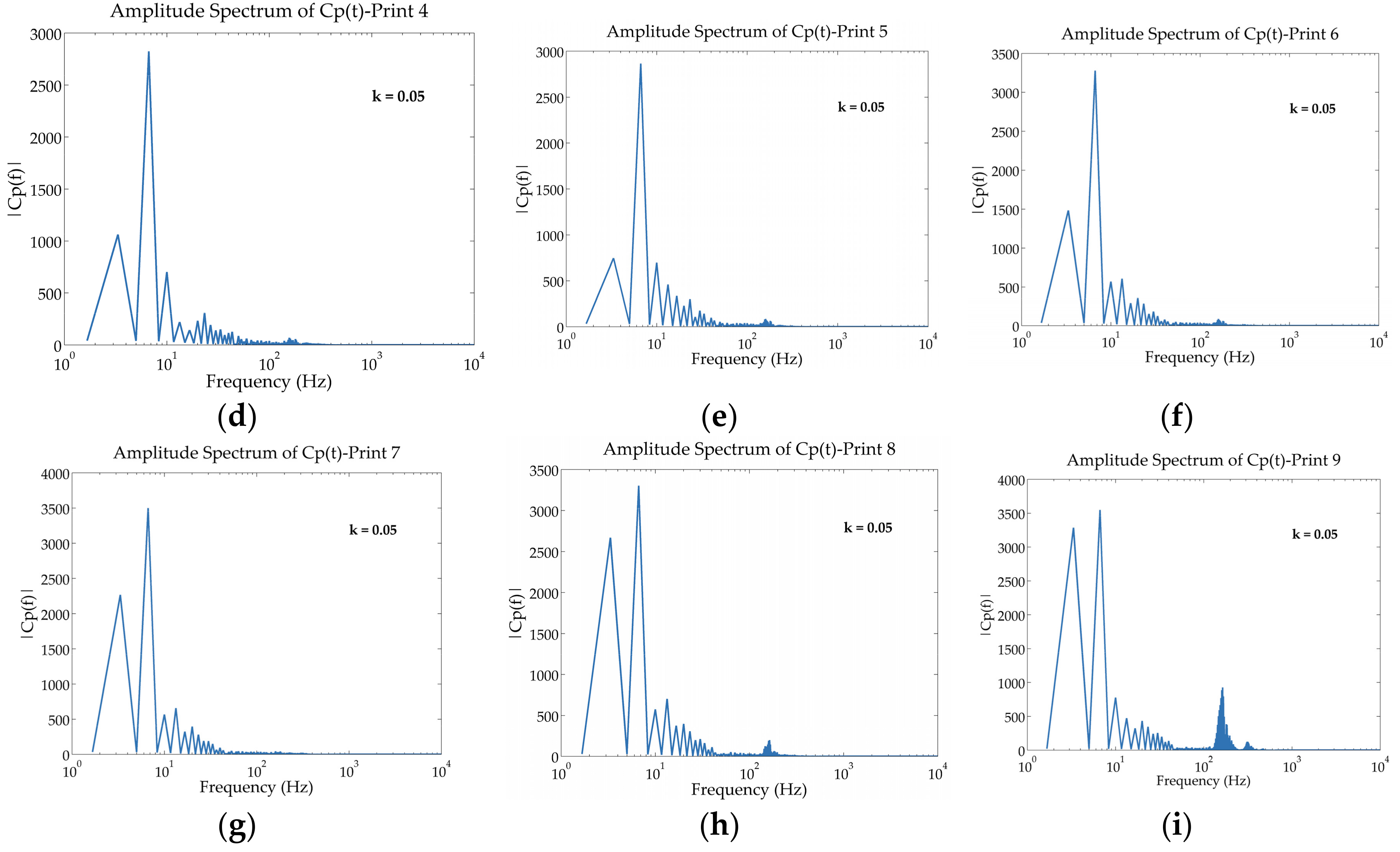
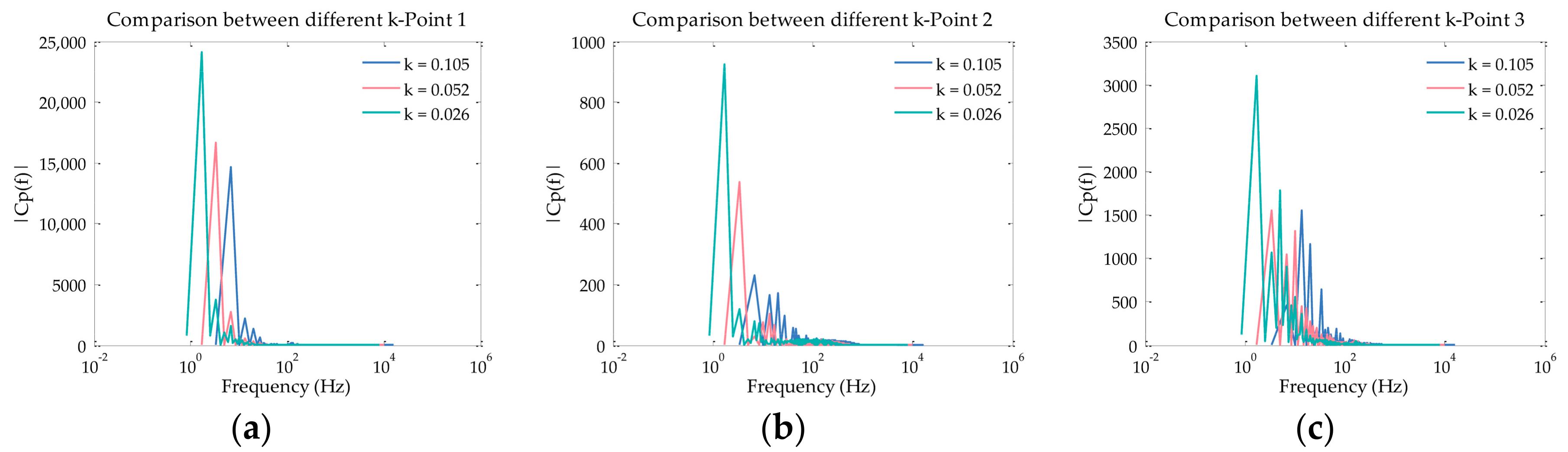
3.3. Frequency Spectrum Analysis of the Pressure Coefficient

The above pressure contours and streamlines can only be observed from a qualitative point of view. This requires multiple consecutive figures to obtain the characteristics of multiple cycles. Instead, spectrum analysis can capture the features of shedding vortices around the airfoil quickly and quantitatively. Spectrum analysis is a technique that converts a complex signal into a set of simple signals with different frequencies. It is a way to find the information (e.g., amplitude, power, intensity or phase, etc.) of a signal at different frequencies. In this paper, nine points are set on the suction surface of the airfoil to collect time series of pressure signals. The positions of the points are shown in Figure 11.

The fast fourier transform (FFT) of the pressure signals was performed with the software MATLAB under different calculations. The spectra of pressure signals were generated by two continuous period signals. Figure 12 shows an example of the time series signals and energy spectrum at Point 6. Figure 12b is the result of Figure 12a after FFT. It shows that the grid in the boundary layer was able to capture small-scale vortices properly, with the turbulence model in the present study.

In order to show the differences between each frequency more clearly, the spectra of surface pressure at all nine points on one airfoil are shown in Figure 13 with the semi-log-x function. The abscissa value at the first peak corresponds to the pitch oscillation frequency f = 3.3333, which can be computed by Equation (4):

$$f=\frac{1}{T}=\frac{1}{2\pi /\omega }=\frac{\omega }{2\pi }= \frac{2U_{\infty }k}{2\pi c}= \frac{U_{\infty }k}{\pi c}$$

(4)

The abscissa value at the second peak corresponds to the vortices’ shedding mode. The flow field around the pitching airfoil consists of large-scale motions and small-scale turbulence motions. The large-scale one has the same time scale as the unsteady pitch oscillations.

By observing the spectra of pressure at the different points on the airfoil in the same case, i.e., k = 0.052, ${\alpha }_0$ = 10°, ${\alpha }_{amp}$ = 10°, it can be seen that most of the energy of the leading edge point, Pt, is concentrated in the first order frequency pitch oscillation. This is because that the pressure signals of the leading edge point basically were affected by the airfoil pitch oscillation and unaffected by shedding vortices. With the position of the points moving backward, the energy of pressure at the second order frequency became higher. This means that the pressure signals begin to be affected not only by the airfoil pitch oscillation, but also by the shedding of vortices. Due to the proximity of the location, the features of Pt 4 and Pt 5 were similar. This was the same for Pt 6 and Pt 7. It is worth noting that the energy of pressure at high frequency $f_v$ = 163.333 at the trailing edge point Pt 9 was much higher than that of other points. This means that there were severe high-frequency fluctuations in the pressure signal at the trailing edge during pitching motion cycles.

By comparing the pressure spectra of the cases with different reduced frequencies, as shown in Figure 14, it can clearly be seen that the vortex shedding frequency increased with the increase of the reduced frequency. At the same time, pressure fluctuations at each point on the airfoil showed different characteristics dependent on reduced frequencies. At the leading edge of the airfoil, the proportion of energy for pressure at the first order of frequency became lower with the increasingly-reduced frequency. This shows that the proportion of pressure variation affected by pitch oscillation and shedding vortex changed. This implies that the increasingly-reduced frequency intensified the unsteady effects. Instead, the change of this proportion was reversed at the trailing edge point. Pitch oscillation played a dominant role in pressure fluctuations with increasingly-reduced frequency at the trailing edge point. The pitch oscillation dominated the fluctuations of pressure signals with k = 0.1, but did not with k = 0.05. This phenomenon provides new evidence of J.G. Leishman’s conclusion that when k is smaller than 0.5, the flow can be considered as quasi-steady [1]. Besides the high-frequency fluctuations in the pressure signal, at the trailing edge during pitching motion, cycles had higher energy, but lower frequency with increasingly-reduced frequency; see Figure 14i.

4. Conclusions

In this paper, in order to better understand the effects of dynamic stall on the aerodynamic characteristics, a CFD method was employed to investigate the influence of the pitch oscillations of the DU 91-W2-250 airfoil. Cases with different reduced frequency were studied by comparing aerodynamic forces and the lift-to-drag ratio. In addition, the hysteresis effect of dynamic stall was analyzed from the perspective of two aspects: the pressure field and spectrum analysis.

The effects of reduced frequency on dynamic stall were analyzed qualitatively and quantitatively. Aerodynamic forces and the lift-to-drag ratio during pitching motion were compared. During the hysteresis loop, the aerodynamic efficiency of the upstroke was lower than that of the downstroke. The effect of delay was more significant with the increased reduction of the frequency. Increasingly-reduced frequency led to lower aerodynamic efficiency during the upstroke process of pitching motions. The result that increasingly-reduced frequency aggravates dynamic stall effects was the same as the conclusions of other observations. Flow field structures and positions of separation points were used to explain the delay of lift stall from other aspects. There were a clockwise-rotating vortex and a counterclockwise-rotating vortex near the trailing edge of airfoil during pitching motions. The growth of the clockwise-rotating vortex increased the value of the lift coefficient, while the growth of the counterclockwise-rotating vortex decreased the value of the lift coefficient.

Frequency spectrum analysis of the pressure coefficient was used as a new method to find the relationship of shedding vortices and pitching motion. The vortex shedding frequency increased with the increase of the reduced frequency. The fluctuations of the pressure signals were the results of pitching motion and vortex shedding. The dominant factor of the pressure signal fluctuations was different at the leading edge and trailing edge. It was also different with different reduced frequencies. Pitch oscillation played a dominant role in pressure fluctuations with increasingly-reduced frequency at the trailing edge point.

In this paper, the dynamic stall characteristics of the DU 91-W2-250 airfoil at $Re=3\times {10}^5$ were analyzed systematically. However, due to the large amount of computing resources and time cost, many problems need to be further studied in the project. For example, a conclusion of this paper was that increasingly-reduced frequency caused angles of attack of stall to increase. However, it is not known yet when will this trend would stop, i.e., what is the biggest reduced frequency to maintain this trend. In addition, dynamic experiments of the DU series airfoil should be carried out as soon as possible to obtain dynamic data for the purpose of verification.

References

1. Leishman, J.G. Principles of Helicopter Aerodynamics; Cambridge University Press: Cambridge, UK, 2006; p. 78. ISBN 9781107013353. [Google Scholar]
2. Holierhoek, J.; De Vaal, J.; Van Zuijlen, A.; Bijl, H. Comparing different dynamic stall models. Wind Energy 2013, 16, 139–158. [Google Scholar] [CrossRef]
3. Choudhry, A.; Leknys, R.; Arjomandi, M.; Kelso, R. An insight into the dynamic stall lift characteristics. Exp. Therm. Fluid Sci. 2014, 58, 188–208. [Google Scholar] [CrossRef]
4. Xiong, L.; Xianmin, Z.; Gangqiang, L.; Yan, C.; Zhiquan, Y. Dynamic response analysis of the rotating blade of horizontal axis wind turbine. Wind Eng. 2010, 34, 543–559. [Google Scholar] [CrossRef]
5. Ham, N.D. Aerodynamic loading on a two-dimensional airfoil during dynamic stall. AIAA J. 1968, 6, 1927–1934. [Google Scholar] [CrossRef]
6. Galvanetto, U.; Peiró, J.; Chantharasenawong, C. An assessment of some effects of the nonsmoothness of the leishman–beddoes dynamic stall model on the nonlinear dynamics of a typical aerofoil section. J. Fluids Struct. 2008, 24, 151–163. [Google Scholar] [CrossRef]
7. Tarzanin, F. Prediction of control loads due to blade stall. J. Am. Helicopter Soc. 1972, 17, 33–46. [Google Scholar] [CrossRef]
8. Tran, C.; Petot, D. Semi-Empirical Model for the Dynamic Stall of Airfoils in View of the Application to the Calculation of Responses of a Helicopter Blade in Forward Flight. Vertica 1981, 5, 35–53. [Google Scholar]
9. Leishman, J.G.; Beddoes, T. A semi-empirical model for dynamic stall. J. Am. Helicopter Soc. 1989, 34, 3–17. [Google Scholar] [CrossRef]
10. Larsen, J.W.; Nielsen, S.R.; Krenk, S. Dynamic stall model for wind turbine airfoils. J. Fluids Struct. 2007, 23, 959–982. [Google Scholar] [CrossRef]
11. Hansen, M.H.; Gaunaa, M.; Madsen, H.A. A Beddoes–Leishman Type Dynamic Stall Model in State-Space and Indicial Formulation; Technical University of Denmark: Lyngby, Denmark, 2004; ISBN 8755030890. [Google Scholar]
12. Gupta, S.; Leishman, J.G. Dynamic stall modelling of the s809 aerofoil and comparison with experiments. Wind Energy 2010, 9, 521–547. [Google Scholar] [CrossRef]
13. Sheng, W.; Galbraith, R.A.M.; Coton, F.N. A modified dynamic stall model for low mach numbers. J. Sol. Energy Eng. 2008, 130, 653. [Google Scholar] [CrossRef]
14. Martinat, G.; Braza, M.; Harran, G.; Sevrain, A.; Tzabiras, G.; Hoarau, Y.; Favier, D. Dynamic Stall of a Pitching and Horizontally Oscillating Airfoil; Springer: Berlin, Germany, 2009; pp. 395–403. [Google Scholar]
15. Wang, S.; Ingham, D.B.; Ma, L.; Pourkashanian, M.; Tao, Z. Numerical investigations on dynamic stall of low reynolds number flow around oscillating airfoils. Comput. Fluids 2010, 39, 1529–1541. [Google Scholar] [CrossRef]
16. Akbari, M.H.; Price, S.J. Simulation of dynamic stall for a naca 0012 airfoil using a vortex method. J. Fluids Struct. 2003, 17, 855–874. [Google Scholar] [CrossRef]
17. Gharali, K.; Johnson, D.A. Dynamic stall simulation of a pitching airfoil under unsteady freestream velocity. J. Fluids Struct. 2013, 42, 228–244. [Google Scholar] [CrossRef]
18. Kim, Y.; Xie, Z.T. Modelling the effect of freestream turbulence on dynamic stall of wind turbine blades. Comput. Fluids 2016, 129, 53–66. [Google Scholar] [CrossRef] [Green Version]
19. Gandhi, A.; Merrill, B.; Peet, Y.T. Effect of Reduced Frequency on Dynamic Stall of a Pitching Airfoil in a Turbulent Wake. In Proceedings of the 55th AIAA Aerospace Sciences Meeting, Grapevine, TX, USA, 9–13 January 2017; p. 0720. [Google Scholar] [CrossRef]
20. Martin, J.; Empey, R.; McCroskey, W.; Caradonna, F. An experimental analysis of dynamic stall on an oscillating airfoil. J. Am. Helicopter Soc. 1974, 19, 26–32. [Google Scholar] [CrossRef]
21. Mccroskey, W.J. Unsteady airfoils. Annu. Rev. Fluid Mech. 2003, 14, 285–311. [Google Scholar] [CrossRef]
22. McCroskey, W.J. The Phenomenon of Dynamic Stall; NASA Ames Research Center: Mountain View, CA, USA, 1981. [Google Scholar] [CrossRef]
23. Wernert, P.; Geissler, W.; Raffel, M.; Kompenhans, J. Experimental and numerical investigations of dynamic stall on a pitching airfoil. AIAA J. 1996, 34, 982–989. [Google Scholar] [CrossRef]
24. Aramendia, I.; Fernandez-Gamiz, U.; Ramos-Hernanz, J.A.; Sancho, J.; Lopez-Guede, J.M.; Zulueta, E. Flow control devices for wind turbines. In Energy Harvesting and Energy Efficiency; Springer: Berlin, Germany, 2017; pp. 629–655. [Google Scholar]
25. Johnson, S.J.; Baker, J.P.; Van Dam, C.P.; Berg, D. An overview of active load control techniques for wind turbines with an emphasis on microtabs. Wind Energy 2010, 13, 239–253. [Google Scholar] [CrossRef]
26. Zhang, L.; Li, X.; Yang, K.; Xue, D. Effects of vortex generators on aerodynamic performance of thick wind turbine airfoils. J. Wind Eng. Ind. Aerodyn. 2016, 156, 84–92. [Google Scholar] [CrossRef]
27. Yang, K.; Zhang, L.; Jianzhong, X.U. Simulation of aerodynamic performance affected by vortex generators on blunt trailing-edge airfoils. Sci. China Technol. Sci. 2010, 53, 1–7. [Google Scholar] [CrossRef]
28. Tsai, K.-C.; Pan, C.-T.; Cooperman, A.M.; Johnson, S.J.; Van Dam, C. An innovative design of a microtab deployment mechanism for active aerodynamic load control. Energies 2015, 8, 5885–5897. [Google Scholar] [CrossRef]
29. Fernandez-Gamiz, U.; Zulueta, E.; Boyano, A.; Ramos-Hernanz, J.A.; Lopez-Guede, J.M. Microtab design and implementation on a 5 mw wind turbine. Appl. Sci. 2017, 7, 536. [Google Scholar] [CrossRef]
30. Barlas, T.K.; Van Kuik, G. Review of state of the art in smart rotor control research for wind turbines. Prog. Aerosp. Sci. 2010, 46, 1–27. [Google Scholar] [CrossRef]
31. Fernandez-Gamiz, U.; Zulueta, E.; Boyano, A.; Ansoategui, I.; Uriarte, I. Five megawatt wind turbine power output improvements by passive flow control devices. Energies 2017, 10, 742. [Google Scholar] [CrossRef]
32. Timmer, W.; Van Rooij, R. Summary of the delft university wind turbine dedicated airfoils. J. Sol. Energy Eng. 2003, 125, 488–496. [Google Scholar] [CrossRef]
33. Bai, J.Y.; Zhang, L.; Xingxing, L.I.; Yang, K. Analyzing the effect of wind tunnel wall on the aerodynamic performance of airfoils. Sci. Sin. 2016, 46, 124707. (In Chinese) [Google Scholar]
34. Poirel, D.; Métivier, V.; Dumas, G. Computational aeroelastic simulations of self-sustained pitch oscillations of a naca0012 at transitional reynolds numbers. J. Fluids Struct. 2011, 27, 1262–1277. [Google Scholar] [CrossRef]
35. Blazek, J. Computational Fluid Dynamics: Principles and Applications, 2nd ed.; Elsevier: New York, NY, USA, 2005; pp. 1–4. [Google Scholar]
36. Hand, B.; Kelly, G.; Cashman, A. Numerical simulation of a vertical axis wind turbine airfoil experiencing dynamic stall at high reynolds numbers. Comput. Fluids 2017, 149, 12–30. [Google Scholar] [CrossRef]
37. Liu, X.; Lu, C.; Liang, S.; Godbole, A.; Chen, Y. Vibration-induced aerodynamic loads on large horizontal axis wind turbine blades. Appl. Energy 2017, 185, 1109–1119. [Google Scholar] [CrossRef] [Green Version]
38. Wang, S.; Ingham, D.B.; Ma, L.; Pourkashanian, M.; Tao, Z. Turbulence modeling of deep dynamic stall at relatively low reynolds number. J. Fluids Struct. 2012, 33, 191–209. [Google Scholar] [CrossRef]
39. Gharali, K.; Johnson, D.A. Numerical modeling of an s809 airfoil under dynamic stall, erosion and high reduced frequencies. Appl. Energy 2012, 93, 45–52. [Google Scholar] [CrossRef]
40. Karbasian, H.R.; Esfahani, J.A.; Barati, E. Effect of acceleration on dynamic stall of airfoil in unsteady operating conditions. Wind Energy 2016, 19, 17–33. [Google Scholar] [CrossRef]
41. Ansys Fluent 14 User’s Guide; Ansys Inc.: Canonsburg, PA, USA, 2011.
42. Durbin, P.A.; Reif, B.P. Statistical Theory and Modeling for Turbulent Flows; John Wiley & Sons: Hoboken, NJ, USA, 2011; ISBN 1119957524. [Google Scholar]
43. White, F.M. Fluid mechanics, 7th ed.; McGraw-Hill: New York, NY, USA, 2011; ISBN 978-0-07-352934-9. [Google Scholar]
44. Raffel, M.; Favier, D.; Berton, E.; Rondot, C.; Nsimba, M.; Geissler, W. Micro-piv and eldv wind tunnel investigations of the laminar separation bubble above a helicopter blade tip. Meas. Sci. Technol. 2005, 17, 1–13. [Google Scholar] [CrossRef]
45. Barakos, G.N.; Drikakis, D. Computational study of unsteady turbulent flows around oscillating and ramping aerofoils. Int. J. Numer. Methods Fluids 2010, 42, 163–186. [Google Scholar] [CrossRef]
46. Martinat, G.; Braza, M.; Hoarau, Y.; Harran, G. Turbulence modelling of the flow past a pitching naca0012 airfoil at 105 and 106 reynolds numbers. J. Fluids Struct. 2008, 24, 1294–1303. [Google Scholar] [CrossRef]
Figure 1. (a) Mesh topology of the whole domain; (b) mesh details near the leading edge; (c) mesh details near the trailing edge.
Applsci 08 01111 g001
Figure 2. Schematic of the pitching movement of the airfoil model.
Applsci 08 01111 g002
Figure 3. Comparison of computed (a) C l and (b) C d with different grid densities during the 4th cycle of pitching motion.
Applsci 08 01111 g003
Figure 4. Comparison of computed C l with different time steps.
Applsci 08 01111 g004
Figure 5. (a) history of the lift coefficient C l ; (b) the repeatability of the lift coefficient C l with k = 0.052, α 0 = 10°, α a m p = 10°.
Applsci 08 01111 g005
Figure 6. Comparison between the numerical results, Rfoil, Xfoil and experimental data [25].
Applsci 08 01111 g006
Figure 7. Comparison of the different reduced frequencies k = 0.105, 0.052, 0.026 of the computed (a) lift coefficient C l , (b) drag coefficient C d and (c) lift-to-drag ratio C l / C d with α 0 = 10°, α a m p = 10°.
Applsci 08 01111 g007
Figure 8. Pressure fields and streamlines for different angles of attack in the pitching cycle with k = 0.052, α 0 = 10°, α a m p = 10°.
Applsci 08 01111 g008
Figure 9. (ai) Vorticity fields and streamlines for different points of angles of attack corresponding to (j) the lift coefficient curve.
Applsci 08 01111 g009aApplsci 08 01111 g009b
Figure 10. Positions of the separation point during dynamic stall with k = 0.052, α 0 = 10°, α a m p = 10°.
Applsci 08 01111 g010
Figure 11. Positions of points to gather the history of pressure signals.
Applsci 08 01111 g011
Figure 12. (a) time series signals and (b) energy spectrum of the pressure coefficient of Point 9 for two periods with k = 0.052, = 10°, α a m p = 10°.
Applsci 08 01111 g012
Figure 13. (ai) Energy spectra of the pressure coefficient at different points on the suction surface of the airfoil in the semi-log-x coordinate system with k = 0.052, α 0 = 10°, α a m p = 10°.
Applsci 08 01111 g013aApplsci 08 01111 g013b
Figure 14. (ai) Comparison of the amplitude spectrum of the pressure coefficient at typical points with different reduced frequencies k.
Applsci 08 01111 g014aApplsci 08 01111 g014b