Article

A Nonlinear Crack Model for Concrete Structure Based on an Extended Scaled Boundary Finite Element Method

1
State Key Laboratory of Coastal and Offshore Engineering, Institute of Earthquake Engineering, Dalian University of Technology, Dalian 116024, China
2
Department of Civil, Architectural and Environmental Engineering, Missouri University of Science and Technology, Rolla, MO 65409, USA
*
Author to whom correspondence should be addressed.
Appl. Sci. 2018, 8(7), 1067; https://doi.org/10.3390/app8071067
Submission received: 27 April 2018 / Revised: 26 June 2018 / Accepted: 26 June 2018 / Published: 29 June 2018
(This article belongs to the Special Issue Computational Methods for Fracture)

Abstract

:
Fracture mechanics is one of the most important approaches to structural safety analysis. Modeling the fracture process zone (FPZ) is critical to understand the nonlinear cracking behavior of heterogeneous quasi-brittle materials such as concrete. In this work, a nonlinear extended scaled boundary finite element method (X-SBFEM) was developed incorporating the cohesive fracture behavior of concrete. This newly developed model consists of an iterative procedure to accurately model the traction distribution within the FPZ accounting for the cohesive interactions between crack surfaces. Numerical validations were conducted on both of the concrete beam and dam structures with various loading conditions. The results show that the proposed nonlinear X-SBFEM is capable of modeling the nonlinear fracture propagation process considering the effect of cohesive interactions, thereby yielding higher precisions than the linear X-SBFEM approach.

Graphical Abstract

1. Introduction

With the development of numerical analysis technology, structural fracture mechanics is an important approach to structural safety evaluation. Fracture process zone (FPZ) is defined as the intermediate space between cracked and uncracked portions of concrete [1]. Different from real cracks, the FPZ can still transmit stress, and the stress, σ, that FPZ transmits decreases with increasing crack open displacement, w. When the crack open displacement reaches a certain critical value, wc, the surface force of the crack surface becomes zero, as illustrated in Figure 1. The FPZ consists of microcracks, which are minute individual cracks; this gives rises to the cohesive tractions ahead of the crack tip, which comes from the aggregate interlocking and surface friction. Therefore, a nonlinear fracture-mechanics-based method needs to be applied to account for the effect of cohesive tractions during the fracture propagations.
Two main approaches are often taken to model the FPZ, which are: the smeared crack models and the discrete crack models. The smeared crack models proposed by Rashid [2] are based on the continuum approach, where the computational mesh of the FPZ remains constant while the fracture propagation is modeled by the growth of a number of parallel cracks smeared over the elements within the FPZ. Using this approach, Bhattacharjee et al. [3] and Calayir et al. [4] successfully carried out dynamic cracking analyses of the Koyna gravity dam under the influence of nonorthogonal cracks. Cai et al. [5] also follow a similar approach incorporating the linear or bilinear softening dispersion crack models to predict the crack response of concrete gravity dams. The damage-based fracture mechanics was also developed sharing the similar concept by Bazant [6]. These methods have shown tremendous success in modeling concrete fractures under complex loading and boundary conditions. However, the strong mesh dependency often causes complications in determining the characteristic length scale, fracture strength, and fracture toughness to accurately describe the fracturing propagation process. The smeared crack models mainly combine with damage mechanics for crack propagation studies.
On the other hand, the discrete crack model proposed by Dugdale [7] and Barenblatt [8] utilizes a predefined fracture path as a part of the computational domain boundary, which reduces the mesh dependency comparing to the smeared crack model. Hillerborg et al. [9] firstly implemented the cohesive zone model (CZM) to describe the FPZ based on the discrete crack approach. Following this approach, numerous scholars have improved and implemented the cohesive zone method to model the fracture propagation process (Skrikerud et al. [10], Ayari et al. [11], Xie et al. and Yang et al. [12,13,14]). Among these improvements, the scaled boundary element method (SBFEM) was developed to model the complex fracture growth in terms of fracture branching and coalescing under complex loading conditions. However, the SBFEM fails to capture the nonlinearity brought by the cohesive interactions within the FPZ. Therefore, the mesoscale and atomic-scale-inserted CZMs were developed to model the FPZ [15,16,17,18]. However, the predetermined fracture paths often cause computational complexities and inaccuracies.
Recently, the extended scaled boundary finite element method (X-SBFEM) based on the level set method was developed on the basis of both the SBFEM [19,20] and the extended finite elements (XFEM) [21,22]. Capitalizing on the advantages of both methods, X-SBFEM [23,24] can make full use of XFEM to describe the discontinuous displacement field and SBFEM to solve the problem of the stress singularity with higher precision. Simulating the crack body section using XFEM and the crack tip using SBFEM, the method finally establishes the total equilibrium equation of the crack body and solves the equation, thereby overcoming the disadvantages of XFEM, such as obtaining the analytical form of the displacement and the stress asymptotic fields of the crack tip in advance and constructing the complex enhanced functions, which can express nonsmooth behaviors near the crack tip. In some special circumstances, the enrichment functions are discontinuous or have nonpolynomial forms to specially address the issue when the stiffness matrix is constructed using numerical integration.
Currently, the application of X-SBFEM in fractures [23] based on linear elastic fracture mechanics (LEFM) mainly focuses on the linear fracture. Due to the complexity of the three-dimensional analysis model, the theoretical researches of fracture mechanics still focus on the state of the two-dimensional analysis model. Therefore, based on the X-SBFEM algorithm, this paper introduces a nonlinear crack model which adopts the linear superposition of iterative methods to incorporate the cohesive interactions within the FPZ. The proposed approach was then implemented to model mixed-mode fracture of concrete beam and gravity dam structures. The results show improvements comparing to other methods. Close agreements were found between the numerical and experimental results.
The contents of this paper are arranged as follows. In Section 2, we explain the principle of X-SBFEM. In Section 3, a nonlinear crack model with iterative method for cohesive interactions in the FPZ is introduced and a flowchart for solving the cohesion is given. In Section 4, four numerical simulations (a three-point bending beam, a four-point shear beam, an experimental concrete gravity dam with single crack expansion, and a static cohesive crack propagation simulation of Koyna Dam) are modeled to validate the nonlinear model. In Section 5, we conclude that this paper has developed the X-SBFEM with the nonlinear model to improve the modeling of crack propagation.

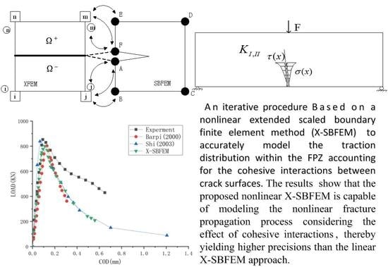
2. Extended Scaled Boundary Finite Element Method

The core content of X-SBFEM based on the level set method focuses on the simulation of the nonsmooth behavior near the crack tip using semianalytical SBFEM in the form of super-elements and the simulation of the crack body using XFEM. The key lies in the way the algorithm addresses the boundary conditions at the joint. Figure 2 below shows the topological relationship in the model domain including a crack based on X-SBFEM.

2.1. Extended Finite Element Method

Based on the partition of unity methods simulating the crack body by XFEM, the general formula of a displacement field [25,26] is
u h ( x ) = I N f e m N I ( x ) q I + J N e N J ( x ) ϑ ( x ) a J
where Nfem and Ne respectively represent a node in a general element and an enriched node in an internal split crack. Correspondingly, q I is a normal degree-of-freedom, a J is a generalized degree-of-freedom related to ϑ (as shown in the square node in Figure 2), and ϑ(x) is the Heaviside step function.
The equilibrium equation is
[ K a a e K a b e K b a e K b b e ] { q I a J } = { P a P b } P b = Ω / Γ d ( H · N ) T · p v d Ω + Γ t ( H · N ) T · t ¯ d Γ + Γ d ( H · N ) T · p d Γ
where K a a e   and K b b e represent the stress matrix respectively related to a normal degree-of-freedom and a generalized degree-of-freedom. Moreover, K a b e and K b a e are the coupling matrices, and P a and P b are the equivalent nodal forces in accordance to general degrees-of-freedom and generalized degrees-of-freedom, respectively.
  K a a e = Ω / Γ d B T D B d Ω
  K a b e = ( K b a e ) T = Ω / Γ d B T D ( H B ) d Ω
  K b b e = Ω / Γ d ( H B ) T D ( H B ) d Ω
  P a = Ω / Γ d N T · p v d Ω + Γ t N T · t ¯ d Γ
  P b = Ω / Γ d ( H · N ) T · p v d Ω + Γ t ( H · N ) T · t ¯ d Γ + Γ d ( H · N ) T · p d Γ
where   Γ d and Γ t   respectively represent the crack face and the force interface. Moreover, p v and t ¯ respectively represent the body force in computational domain and the surface force on the force interface.
According to the advantage of the description of discontinuous displacement field description, XFEM is used to simulate the main body of the crack.

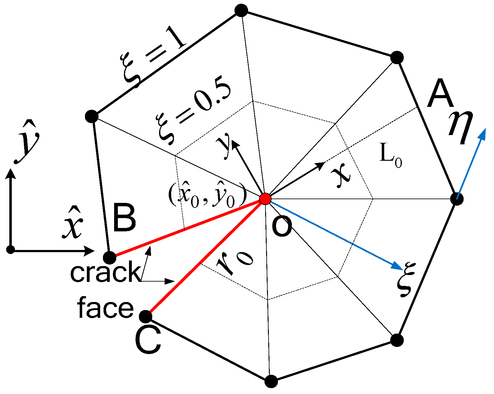
2.2. Scaled Boundary Finite Element Method

X-SBFEM is used to simulate the crack tip for the high efficiency and high precision of stress singular field simulations. As shown in Figure 3, there are side-face forces at the face of the super-element at the crack tip in the case of SBFEM. Without taking the body force into account, the displacement field and the stress field given by the SBFEM are [21]
  { u ( ξ ,   η ) } = [ N ( η ) ] { u ( ξ ) } = i = 1 n c i ξ λ i [ N ( λ ) ] { φ i }
  { σ ( ξ ,   η ) } = [ D ] [ L ] [ N ( η ) ] { u ( ξ ) } = [ D ] [ B 1 ( η ) ] { u ( ξ ) } , ξ + 1 ξ [ D ] [ B 2 ( η ) ] { u ( ξ ) }
where N ( η )   is the interpolation shape function for one-dimensional line elements and { φ i }   and λ i are the displacement modes and the eigenvalues, respectively. Furthermore, [ B 1 ( η ) ] and [ B 2 ( η ) ] are determined by the geometric shape of the boundary of the element. The formulas calculated by the virtual work principle are
  { P } = [ K ] { u h } = [ E 0 ] [ Φ ] [ λ ] [ Φ ] 1 + [ E 1 ] T { u h }
  [ E 0 ] ξ 2 { u ( ξ ) } , ξ ξ + ( [ E 0 ] + [ E 1 ] T [ E 1 ] ) { u ( ξ ) } , ξ [ E 2 ] { u ( ξ ) } = 0
where { P } is the equivalent boundary nodal force and [ E 0 ] , [ E 1 ] , and [ E 2 ] are the coefficient matrices of the SBFEM governing equations.
Equation (11) is a second-order homogeneous ordinary differential equation and its solution is
  { u ( ξ ) } = [ Φ ] ξ λ { c } = i = 1 n c i ξ λ i φ i
where c i is the weight of this mode.
Substitute Equation (12) into Equation (10) and get a quadratic eigenvalue problem.
      [ λ i 2 [ E 0 ] + λ i ( [ E 1 ] T [ E 1 ] ) [ E 2 ] ] φ i = 0
Substitute Equation (12) into Equation (10) and get the equivalent node force q i   on the boundary corresponding to the displacement mode.
    q i = ( [ E 1 ] T + λ i [ E 0 ] ) i
Combining Equations (13) and (14) and introducing auxiliary variables can transform quadratic eigenvalue problems into standard linear eigenvalue problems.
      [ [ E 0 ] 1 [ E 1 ] T [ E 0 ] 1 [ E 1 ] [ E 0 ] 1 [ E 1 ] T + [ E 2 ] [ E 1 ] [ E 0 ] 1 ] [ Φ Q ] = λ [ Φ Q ]
where [Φ] and [ Q ] are modal matrices of the displacement modal matrix and the force modal matrix.
For the square root singular problem for homogeneous materials, the stress intensity factors can be defined as
  { K I K I I } = 2 π L 0 = i = 1 , 2 ( c i { ψ y y ( η = η A ) ψ x y ( η = η A ) } i )
where L0 is the distance between the scaling center and the point of the crack surface (the segment OA in Figure 3). From Equation (8), it can be deduced that if λ i   1 , the distribution of the stress mode tends to 0 when ξ 0   [27].

2.3. Force Balance and Displacement Coordination

Figure 4 shows a typical method simulating the crack with the coupling of the XFEM and the SBFEM [28] domain. In the process of XFEM and X-SBFEM coupling, there is a problem of the balance of virtual and real freedom, continuous displacement, and force. To solve the problem, the SBFEM simulates the crack surface using the boundary of the element, while the XFEM introduces an additional degree-of-freedom based on the use of the step function to describe the discontinuous displacement field. To coordinate the displacement of the two types of elements along the boundary, a transition matrix T is used to match the nodal displacements in SBFEM with those in XFEM. A transformation matrix, which can be derived from the previous equations that translates the unknown SBFEM nodal displacements (uE, uF, uA, and uB) to the unknown XFEM nodal displacements (q2, q3, a2, and a3) can be described as
{ u B u E u A u F } = [ I 0 0 0 0 I 0 0 N 2 ( x A ) N 3 ( x A ) 0 2 N 3 ( x A ) N 2 ( x F ) N 3 ( x F ) 2 N 2 ( x F ) 0 ] { q 2 q 3 a 2 a 3 }
where I is a unit matrix. In order to ensure the compatibility of the displacement and to integrate the element stiffness matrix, it is necessary to rearrange the column displacement vectors of the SBFEM and the stiffness matrix according to whether the nodes are on the common boundary,
  [ K a a K a b T T K b a T T K b b T ] { u q S u x F } = { F a T T F b }
where the subscript a represents the nodes on the common boundary of SBFEM and XFEM and subscript b represents the nodal degree-of-freedom of the noncommon boundary. The transformation matrix T is only related to the interpolation shape function at the crack opening at the common boundary of the SBFEM and the XFEM.

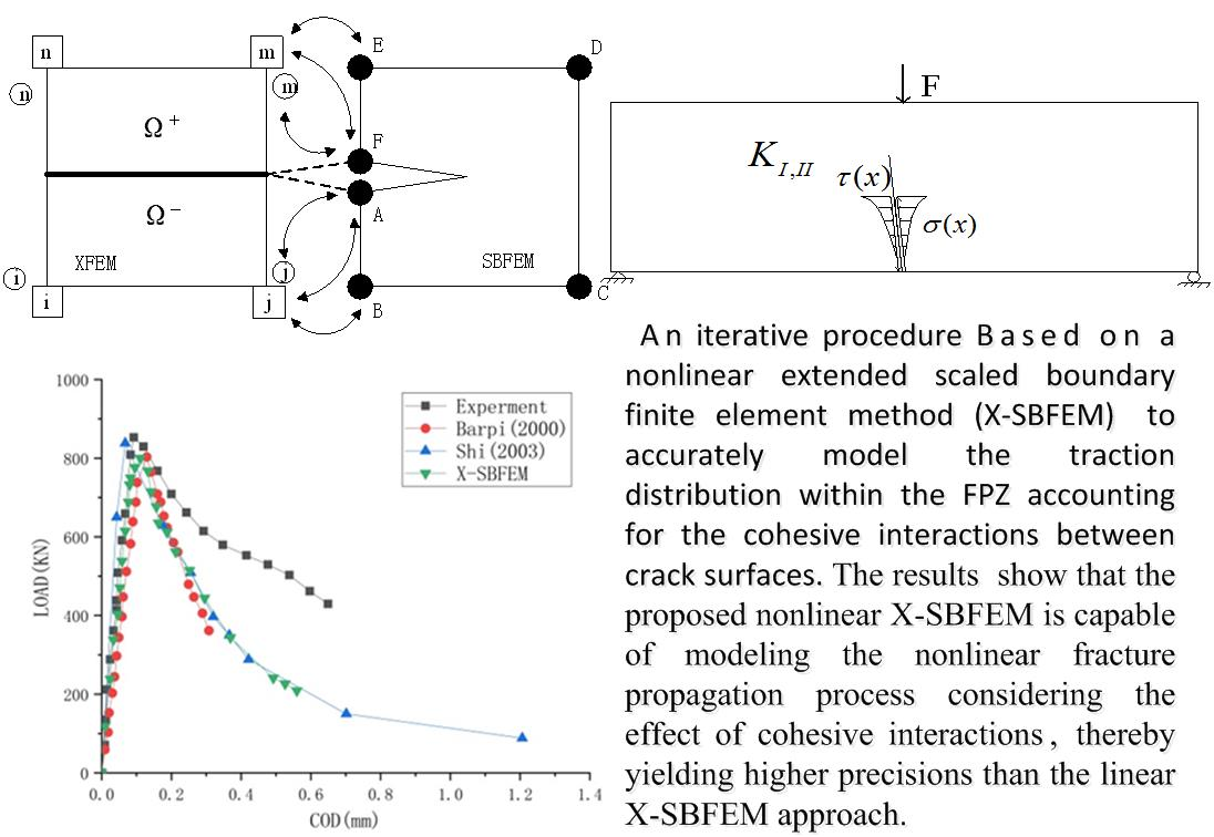
3. A Nonlinear Crack Model with Iterative Method for Cohesive Interactions in the FPZ

The relative displacement of the crack surface, including the opening displacement (COD) and the sliding displacement (CSD) of the crack surface, does not exceed the limits shown in Figure 5. When the COD and CSD of the crack surface are not beyond the limits shown in Figure 5, the total loads generated by the structure include the external loads and the cohesive forces at the virtual crack surfaces. However, if the load exceeds the limit, the cohesive force is 0. In the case of cohesive forces, considering the stress intensity factor I as an example, the stress intensity factor consists of two parts [29],
  K I =   K I P + K I C
where K I is the total stress intensity factor and K I P and K I C are the components related to the external and cohesive forces, respectively. All three stress intensity factors can be calculated by the standard SBFEM solution stress intensity factor formula. Thus, K I P > 0 when the crack opens as a result of the external force of the model, while K I C < 0   when the crack tends to close owing to the cohesive force. Equivalently, K I = 0   when force balance is achieved as a result of the roles of the external and cohesive forces. Therefore, K I 0   can be used as the criterion for judging whether the crack will continue to propagate or not [15].
The positive component of the cohesive tractions in the fracture process zone is determined by the bilinear softening curve [30] of Figure 5a or the linear softening curve of Figure 5b. The tangential component is determined by the curve of Figure 5c. The areas below the curve of Figure 5a,b are the mode I fracture energy,   G f I . The area between the curves in Figure 5c is twice that of the mode II fracture energy,   G f I I [30]. The key concept of this method is based on the relative displacement of the crack surface and its application to the linear superposition of an iterative scheme to solve and estimate the cohesive tractions on the crack surface. Specifically,
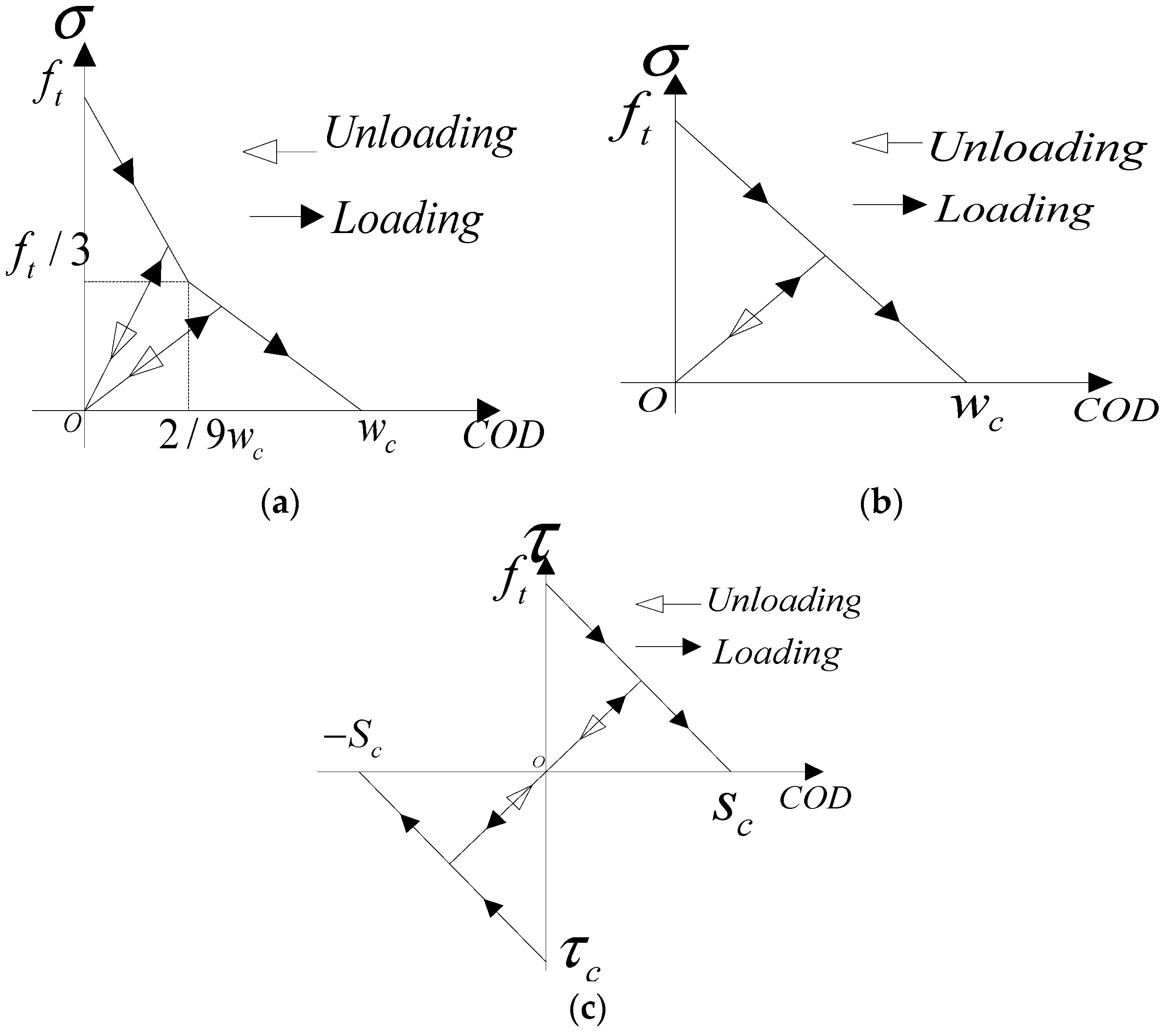
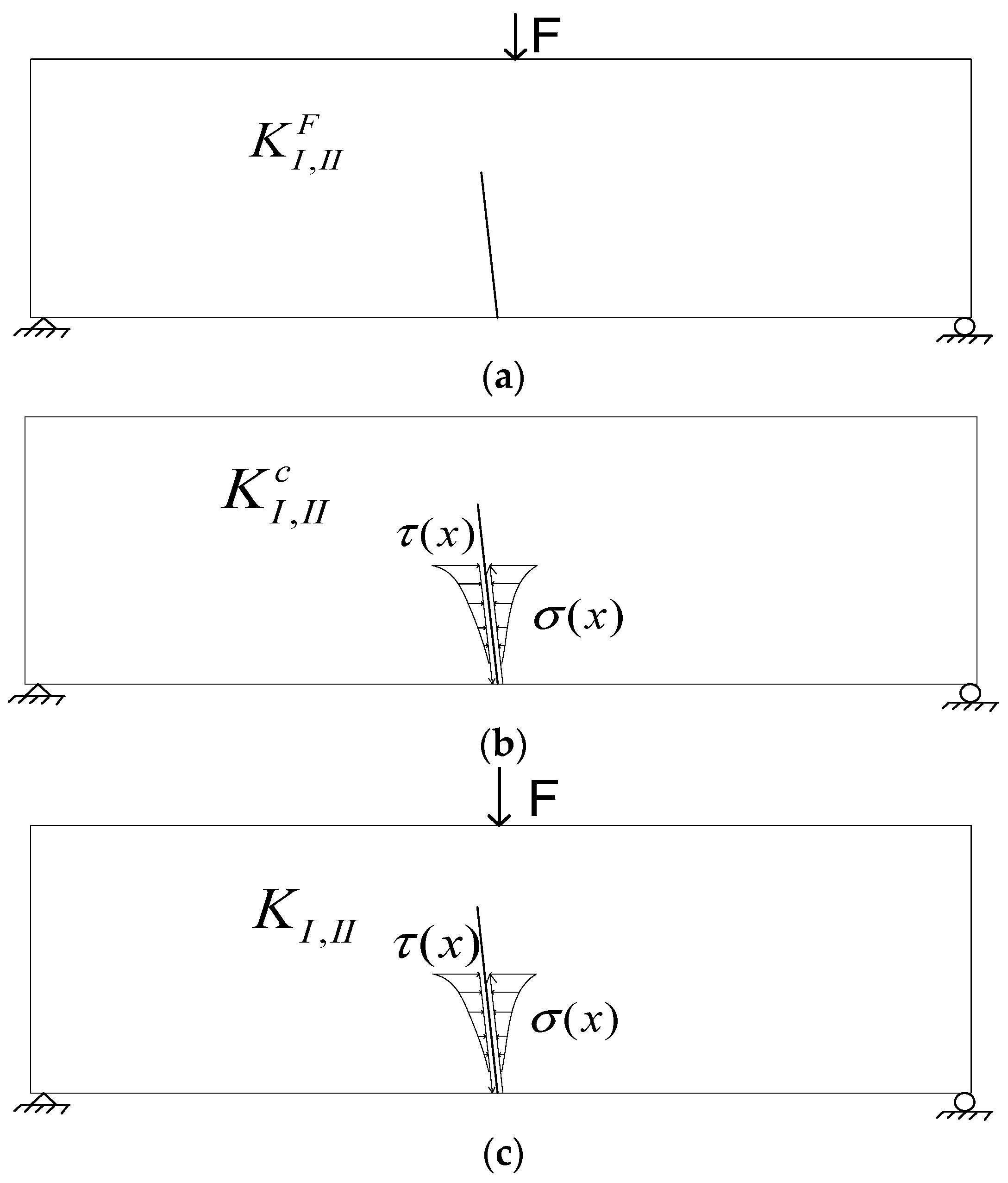
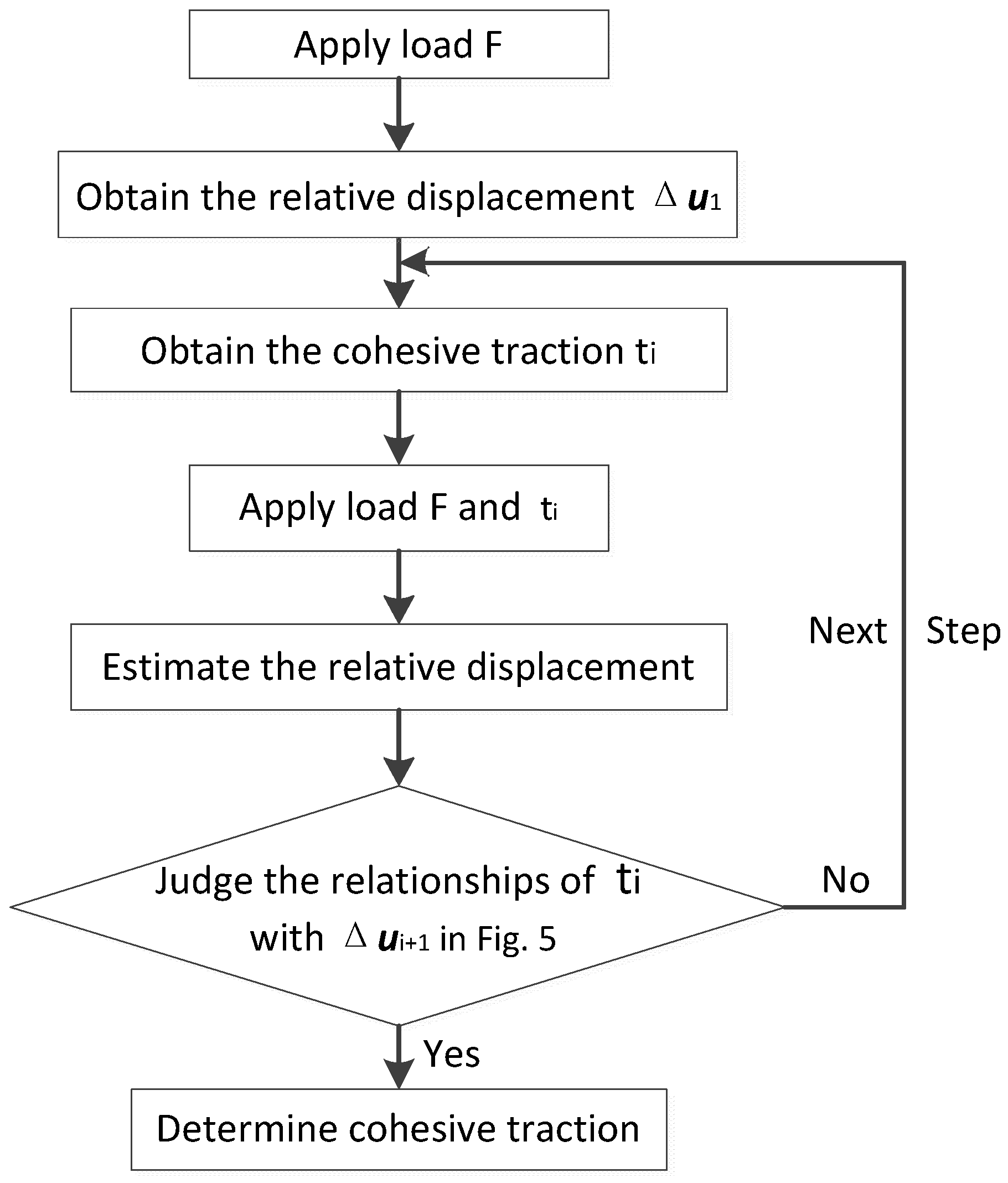
  • Assume that the structure is only affected by the external force so that the relative displacement Δ u 1   of the super-element crack surface Δ u 1   can be obtained based on the linear elastic assumptions of X-SBFEM, and that the corresponding cohesive traction t 1 can be obtained according to Figure 5.
  • As shown in Figure 6, the external force and the cohesive force obtained in the previous step are applied to the structure, wherein the cohesive traction t 1 is applied in the form of a side-face force, formulated in accordance to the following equation:
      S { δ u ( ξ , η ) } T { p n ( ξ ,   η ) } d S = 0 1 { δ u ( ξ ) } T { p n ( ξ ) } x ( ξ ) 2 + y ( ξ ) 2 d ξ   =   0 1 { δ u ( ξ ) } T F t ( ξ ) d ξ
    where
      F t ( ξ ) = { x 1 2 + y 1 2 { p n ( ξ ) } | η = 1 x 1 2 + y 1 2 { p n ( ξ ) } | η = 1 }
The SBFEM nonhomogeneous control equation can be easily obtained in accordance to
  [ E 0 ] ξ 2 { u ( ξ ) } , ξ ξ + ( [ E 0 ] + [ E 1 ] T [ E 1 ] ) { u ( ξ ) } , ξ [ E 2 ] { u ( ξ ) } + ξ { F t ( ξ ) } = 0
Assume that the load can be expressed by the power series,
  { F t ( ξ ) } = i = 1 n ξ t i { F t i }
The corresponding displacement mode is
  { u t ( ξ ) } = i = 1 n ξ t i { Φ t i }
Substituting Equation (24) into Equations (23) and (11) results in
  { Φ t i } = [ ( t i + 1 ) 2 [ E 0 ] + ( t i + 1 ) [ [ E 1 ] T [ E 1 ] ] [ E 2 ] ] 1 { F t i }
  { q t i } = [ ( t i + 1 ) [ E 0 ] + [ E 1 ] T ] { Φ t i }
Thus, the complete displacement of the boundary nodes and the equivalent nodal force are respectively,
  { u h } = i = 1 n { Φ t i } + [ Φ ] { c }
  { P } = i = 1 n { q t i } + [ Q ] { c }
[Φ] and [ Q ] are modal matrices of the displacement modal matrix and the force modal matrix solved by Equation (15), respectively. The following equation can be obtained using Equations (27) and (28):
  [ K ] { u h } = { P } i = 1 n { q t i } + [ K ] i = 1 n { Φ t i }
The equivalent nodal force of the super-element boundary node generated by the distributed load of the crack surface is
  R F = i = 1 n { q t i }   + [ K ] i = 1 n { Φ t i }
When the crack tip is solved characteristically, { u s b h   } and { u x f   } can be obtained after solving the linear equations. Substituting { u x f   } into Equation (17), the displacement of all nodes in the crack tip of the super-element { u s b h   } can be obtained. Substituting { u s b h   } into Equation (27) yields
  { c } = [ Φ ] 1 ( { u s b h   } { Φ t } )
The displacement field of the crack tip element is
  { u ( ξ , η ) } = N ( η ) ( i = 1 n c i ξ λ i { φ i } ξ t + 1 { Φ t } )
where { ψ i } is the stress mode solved based on SBFEM. The relative displacement Δ u i + 1 is solved using Equation (32).
C.
Repeat the steps until the relationship between t i and Δ u i + 1 becomes consistent with the pattern of variation plotted in Figure 5.
A simplified flowchart of the solution of the cohesive tractions is shown in Figure 7.

4. Numerical Examples

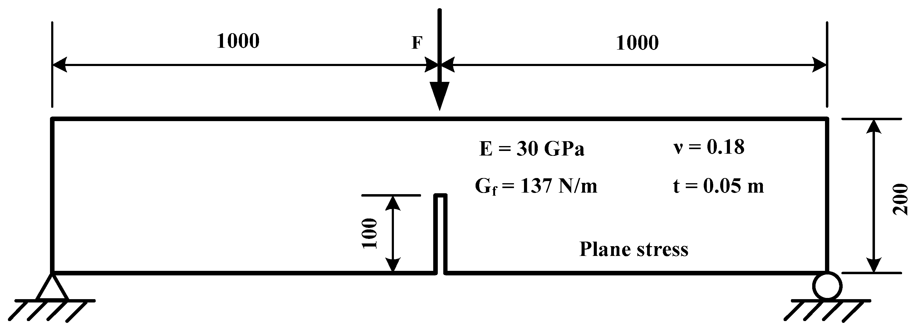
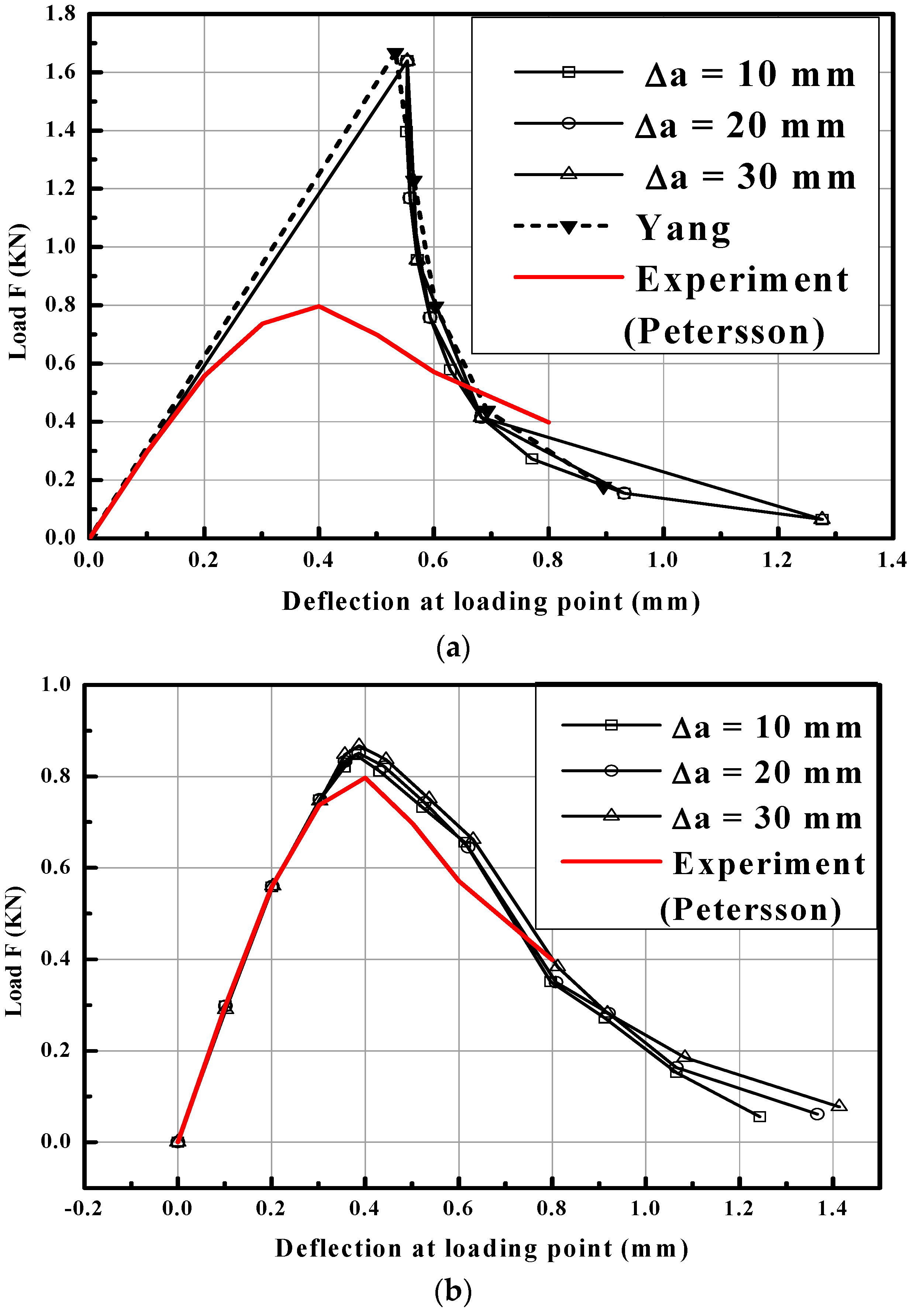
4.1. A Three-Point Bending Beam

This model was first studied by Petersson (1981) as an experimental study of the mode I fracture propagation problem [31]. The geometry, boundary conditions, and material parameters of the beam are shown in Figure 8. The tensile strength f t   is 3.33 MPa and the mode I fracture energy   G f I is 137 N/m. The present example predicts the crack propagation path based on the LEFM maximum circumferential tensile stress criterion. Analyzing the single linear softening curve (Figure 5b) and based on the mode I fracture energy   G f I , the limit value of the linear softening curve w c is 0.0823 mm. The results of three crack propagation steps a = 10 mm, 20 mm, and 30 mm, for a 20 × 200 grid density, are calculated and compared with the results based on the linear elasticity method [24].
Figure 9a depicts the relationship of the load for three different crack propagation steps and load point displacements (Load–LPD) based on LEFM work. The results are compared with Yang’s work based on the linear elasticity method [12] and experimental results published by Petersson [27], as shown in Figure 9. We can see that the elicited results based on LEFM are very different from the experimental data. This is particularly evident for the peak load, which is much higher than the experimental peak. This is because the LEFM-based method is incapable of simulating the energy dissipation of the fracture zone. Based on X-SBFEM, this study has used different methodologies to solve the cohesive tractions based on the iterative method of linear superposition by simulating the energy dissipation of FPZ. Figure 9b shows the Load–LPD curves for three different crack propagation steps considering FPZ nonlinearities. It can be seen from Figure 9 that the calculated results are in good agreement with the experimental results of Petersson, which shows that the method used in this study can simulate the energy dissipation of FPZ. Moreover, it can be seen from Figure 9 that the results of the three crack propagation steps are in good agreement with the experimental curve, which shows that different steps have minor effects on the calculated results.

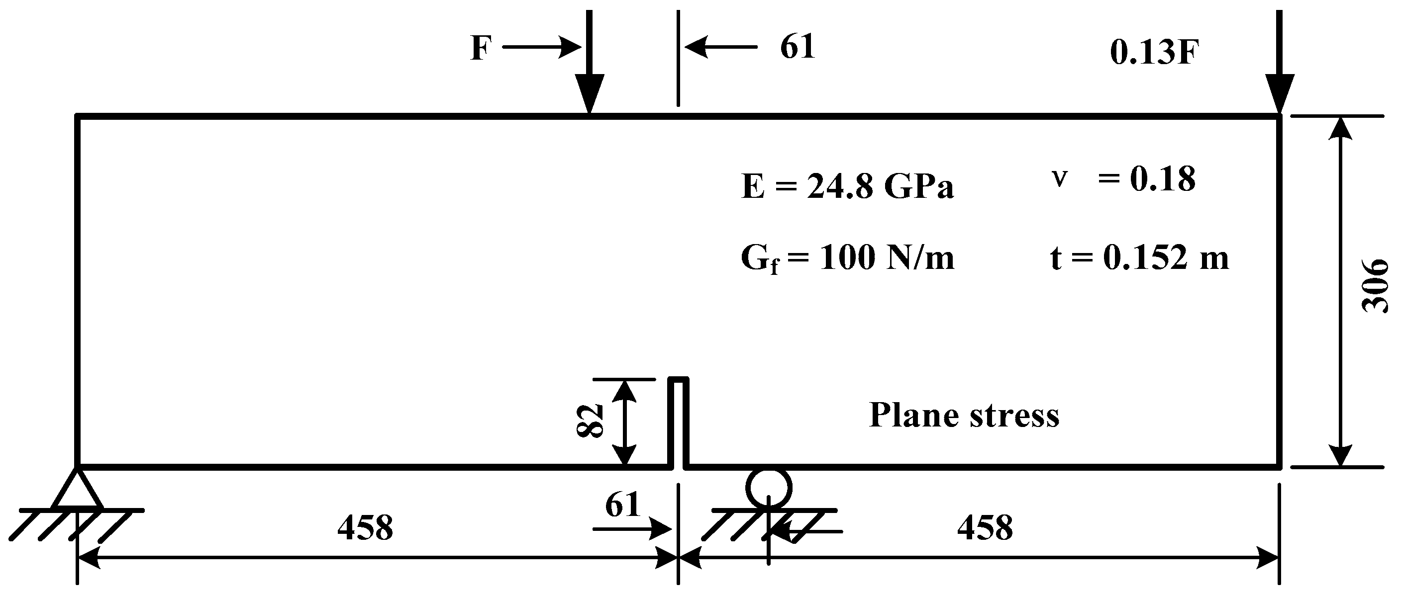
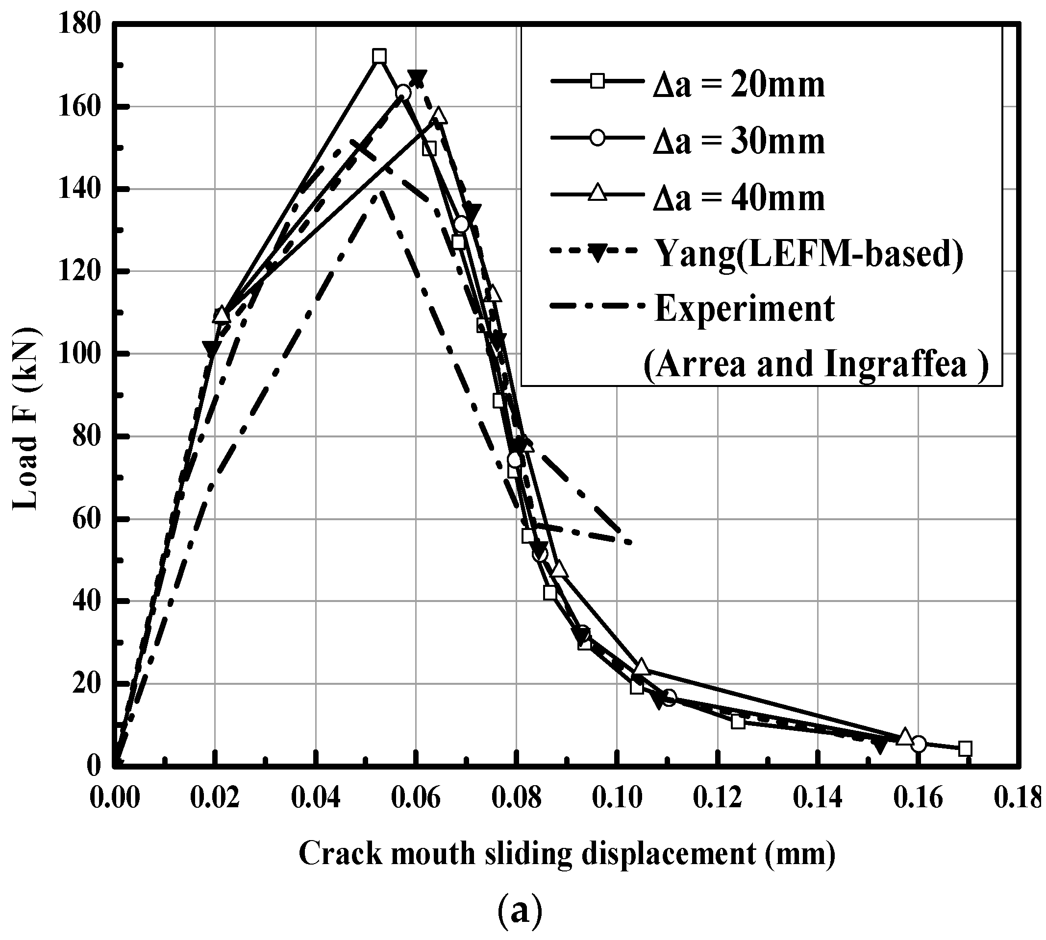
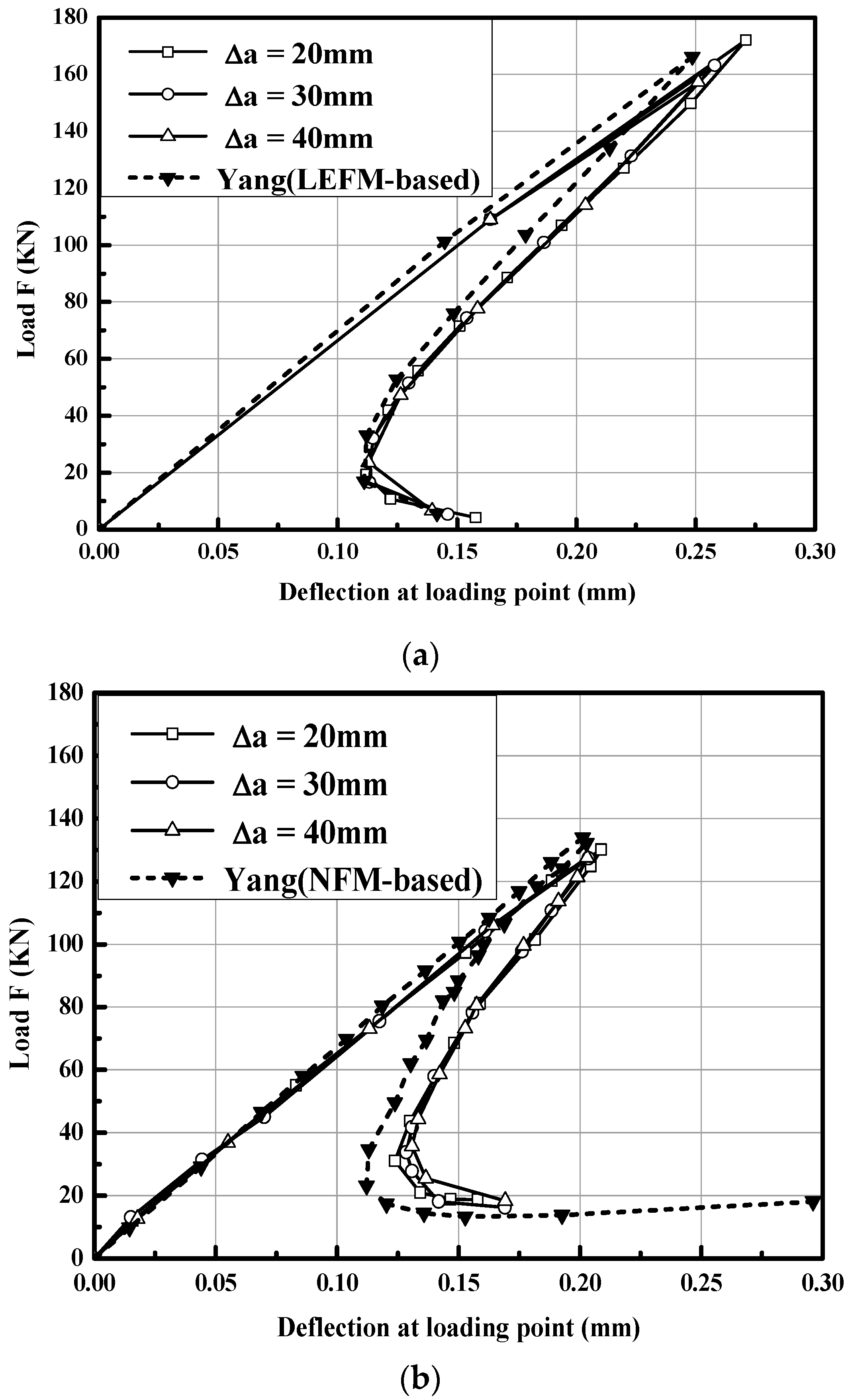
4.2. A Four-Point Shear Beam

Arrea and Ingraffea first tested and analyzed the four-point unilateral shear beam [28]. The geometry and boundary conditions of the beam are shown in Figure 10. Assuming that the structure is in the plane stress state, the Young’s modulus E is 24.8 GPa, Poisson’s ratio υ is 0.18, tensile strength f t is 3.0 MPa, mode I fracture energy   G f I is 100 N/m, and mode II fracture energy   G f I I is 10 N/m. The crack path is also predicted by using the LEFM-based maximum circumferential stress criterion. Analyzing the linear softening curve of Figure 5b, the limit value of CODs w c obtained by the mode I fracture energy   G f I   is 0.067 mm and the limit value of CSDs s c obtained by the mode II fracture energy   G f I I is 0.02 mm. The results of the three crack propagation steps a = 10 mm, 20 mm, and 30 mm, using a 20 × 200 grid density, are calculated and compared with the results based on the linear elasticity method [24].
Figure 11a and Figure 12a show the relationship between the load calculated by LEFM, the crack mouth sliding displacement (Load–CMSD), and the relationship between the load and the loading point displacement (Load–LPD). It can be seen from the figure that the calculated results are close to the numerical solutions of Yang et al. [12] and the effect of different steps on the calculation results is not considerable, which proves the applicability of the X-SBFEM algorithm to complex crack propagation problems. However, the FPZ energy dissipation of the crack tip makes the LEFM-based method slightly different compared to previous calculations and experimental data [15]. In this study, the iterative method used to simulate the cohesive tractions is used to simulate the energy dissipation of the FPZ. The linear softening curve in Figure 5b and the curve of Figure 5c are used to solve the cohesive tractions of the vertical crack surface and the parallel crack surface. As shown in Figure 11b, it can be seen that the Load–CMSD curve calculated herein is in good agreement with Yang’s experimental data (NFM-based). Figure 12b shows that the method considered herein can describe the snap-back phenomenon of the Load–LPD curve. It can be concluded that the iterative, linear superposition method based on X-SBFEM can yield high-precision results without coupling the interface unit (CIEs) near the crack tip.

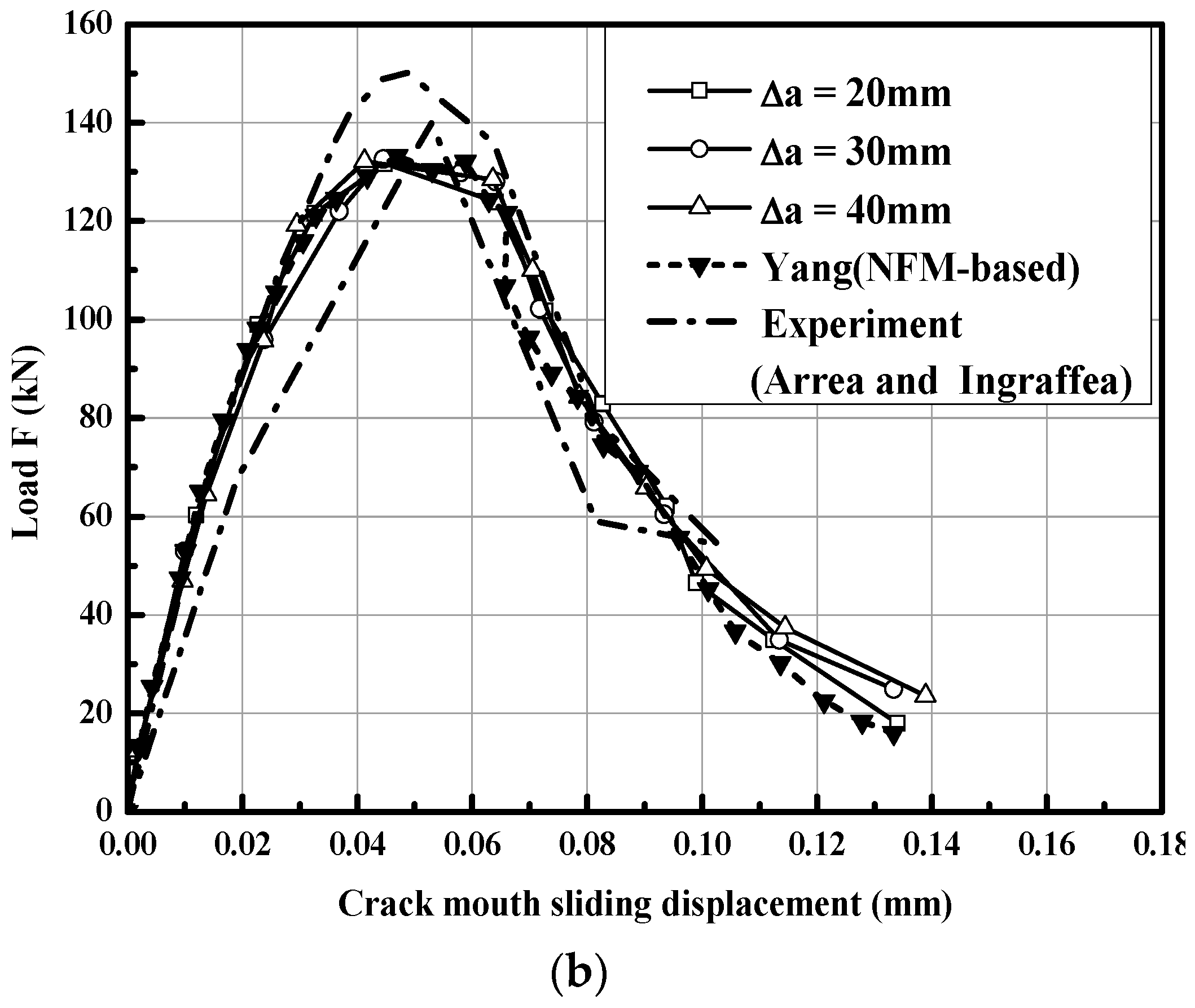
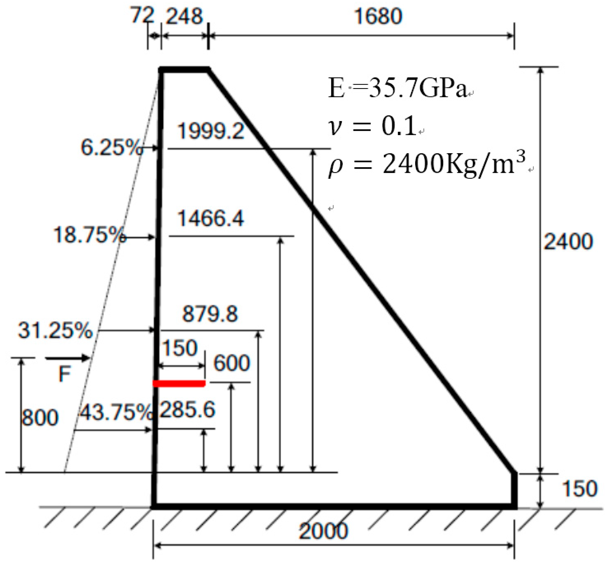
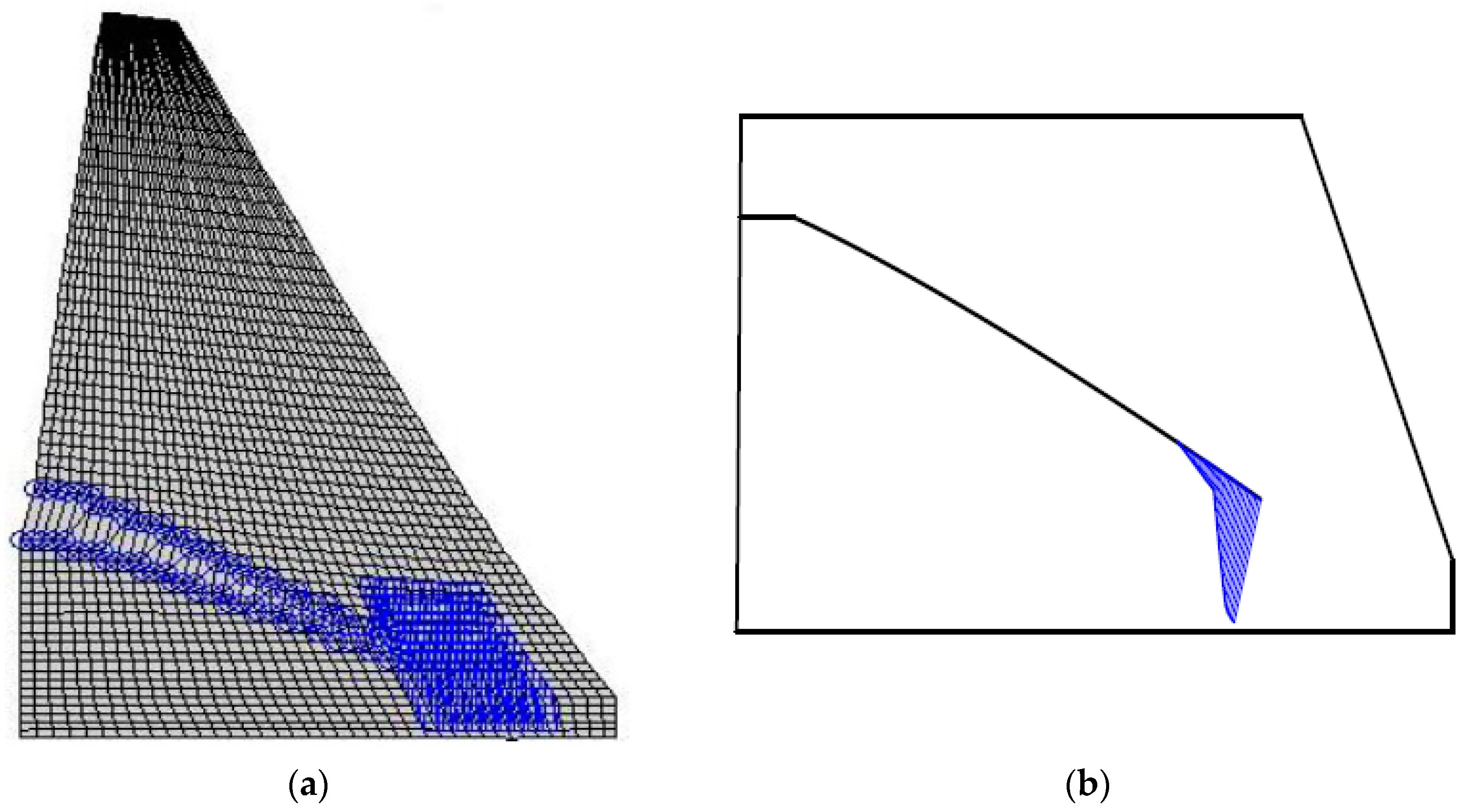
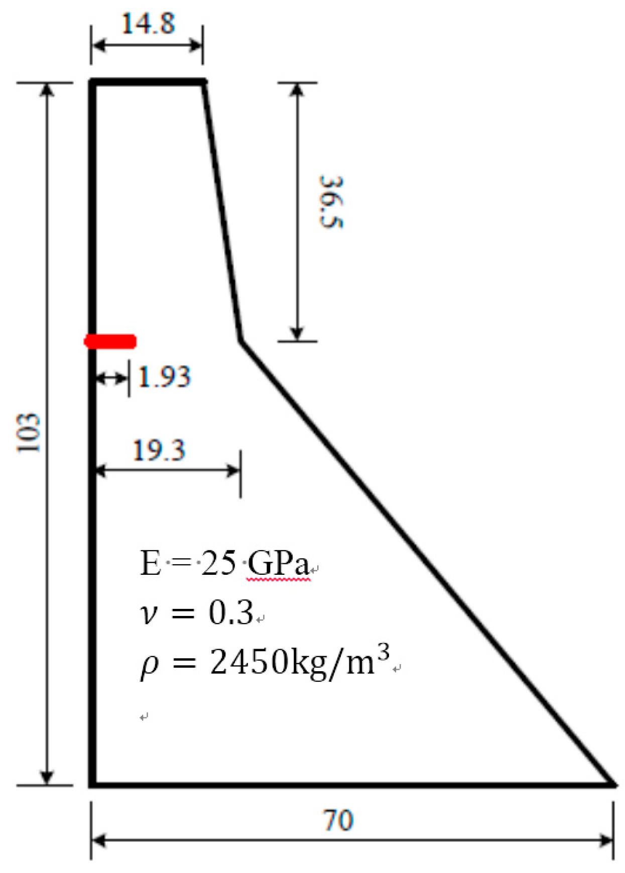
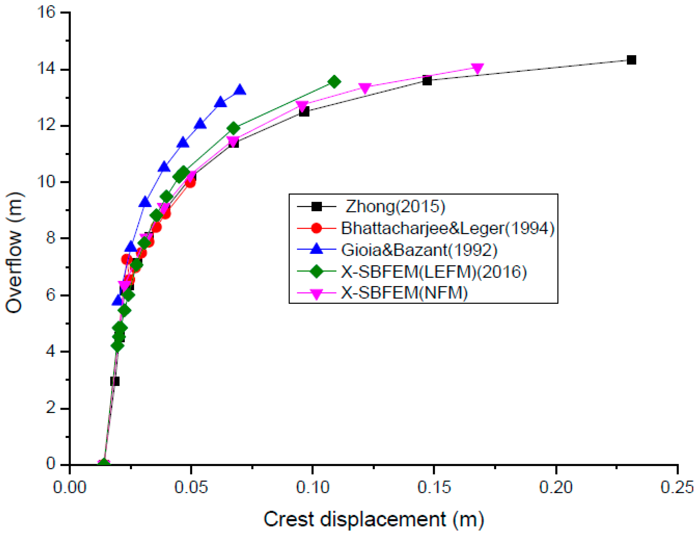
4.3. An Experimental Concrete Gravity Dam with Single-Crack Expansion

Carpinteri [32], Barpi [33], and Shi [34] tested and analyzed the single-crack expansion gravity dam. A 1:40 scale concrete gravity dam model is used herein. The geometry, boundary conditions, and material parameters of the gravity dam are shown in Figure 13. Consisting of concrete, the gravity dam is analyzed based on a plane strain assumption and on the bilinear softening curve, where ω c = 0.256   mm , Gf = 184 N/m, and ft = 3.6 MPa. Suppose that the indentation length is 1/10 W (0.15 m), where W is the width of the dam at the elevation of the indentation. Hydrostatic pressure exists in the upstream face of the dam. This hydrostatic pressure acts on the upstream face and can be equivalently replaced by four concentrated loads, as shown in Figure 13. The hydrostatic pressure gradually increases until the dam breaks.
In Figure 14, the results of the Load–COD curve in this study are compared with reference solutions, the experimental data of Carpinteri et al. [32], and the numerical simulation data of Barpi et al. [33] and Shi et al. [34]. It can be seen that the elicited results before the peak, load peak, and experimental data obtained by this method are in good agreement with all the other numerically elicited data. It can also be seen that the post-peak curve of the experiment was significantly higher than the numerical results, which means that the crack opening displacement (COD) of the experiment was greater under the same loading conditions. This phenomenon may be owing to the unanticipated rigid rotation in the experiment of Carpinteri et al. [32] which results in premature failure of the prefabricated crack. Compared with other numerical results shown in Figure 14a, the initial stiffness obtained by the X-SBFEM method in this study is the closest to that obtained from the results of Carpinteri et al. [32]. The results obtained by Barpi et al. [34] were smoothened before the peak, while the large stiffness elicited in the pre-peak response obtained by Shi et al. [35] resulted in a crack opening displacement (COD) that was smaller in value compared to the experimental results.
The crack trajectories obtained by the above experiment and numerical method are shown in Figure 14b. The crack trajectory obtained by the X-SBFEM method in this study is better matched with the experimental and with all the other numerical results. Among them, the crack trajectory obtained from the experiment directly developed towards the dam site before the dam ruptured. At the same time, the trajectories obtained by the numerical simulations of Barpi et al. [33] and Shi et al. [34] horizontally penetrated the dam body, which is quite different compared to the experimental results. The results generated in this study obviously match more closely the experimental results.
Figure 15 shows the variation of the crack opening displacement and the distribution of cohesive traction with the crack path in this example model, based on the X-SBFEM method.

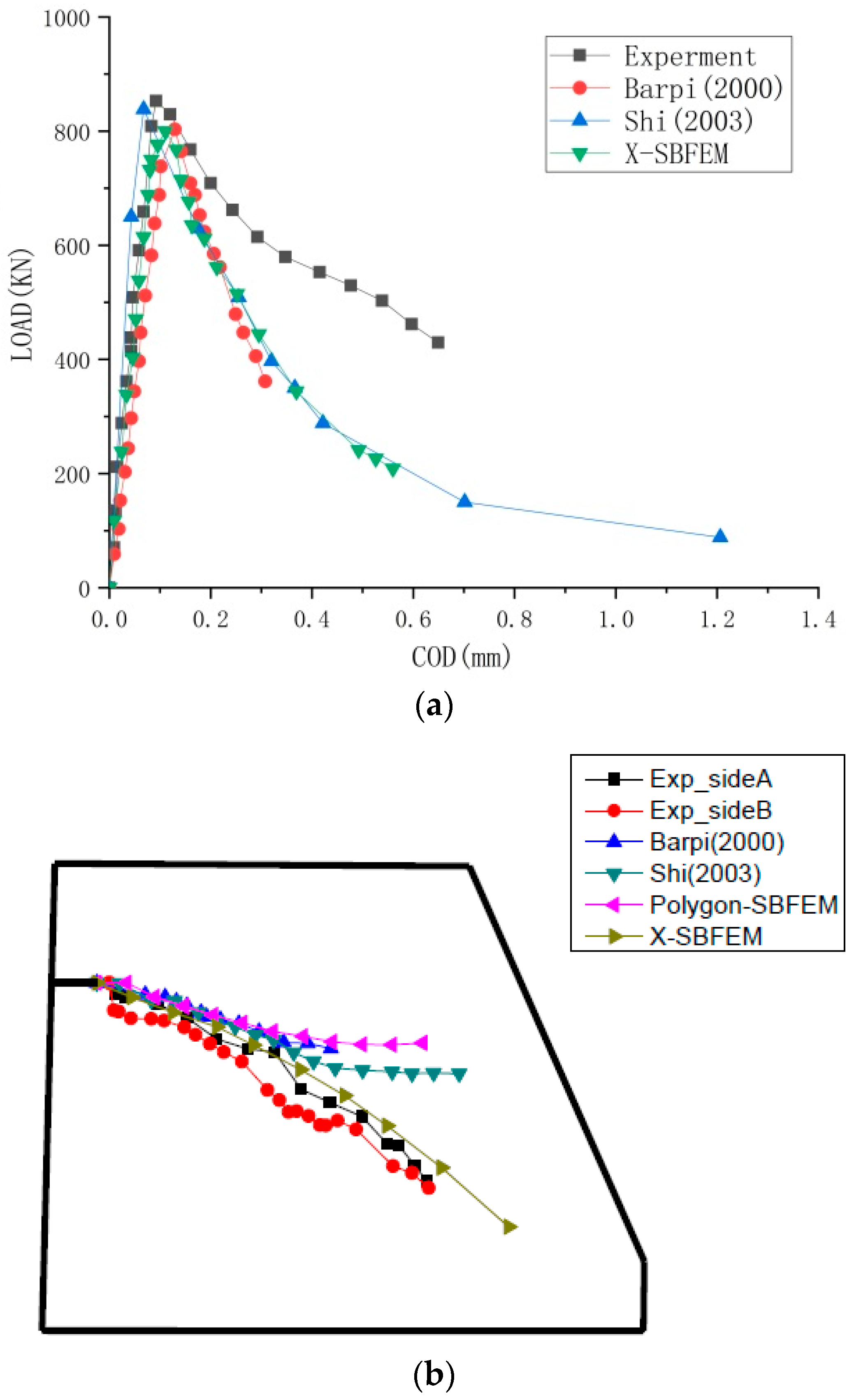
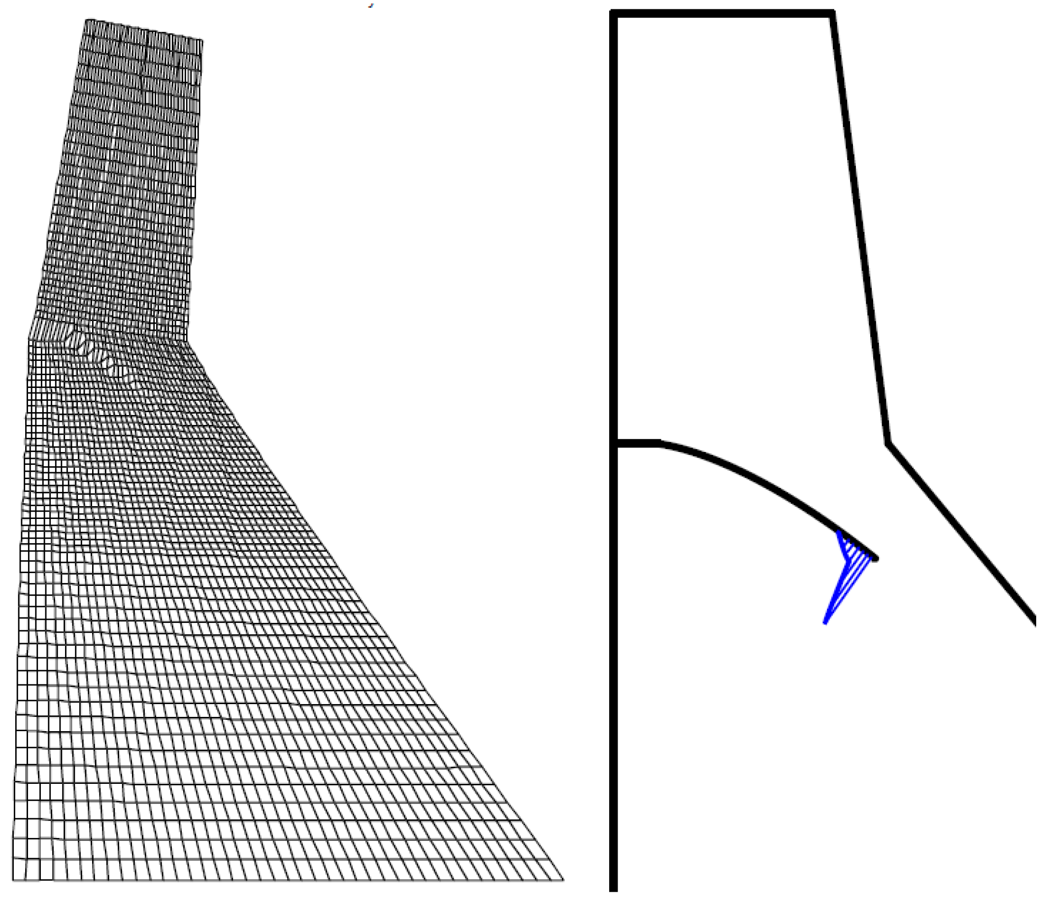
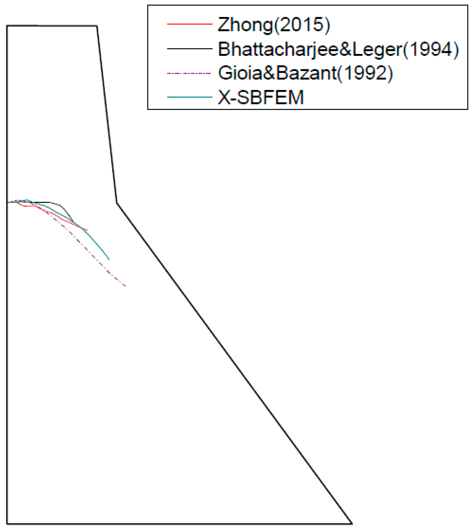
4.4. Static Cohesive Crack Propagation Simulation of Koyna Dam

After a severe earthquake in 1967, the neck of the Koyna Dam suffered serious damages. Gioia et al. [35] (1992) simulated the generated crack based on linear elastic fracture mechanics and Bhattacharjee et al. [36] applied the smeared model to analyze the crack propagation. The geometry and material parameters of the Koyna Dam are shown in Figure 16. The dam concrete was assumed to be homogeneous and the Koyna Dam was analyzed based on the planar strain assumption and the bilinear softening curve, where ω c = 0.256   mm , ω 0 = 0.04   mm , ω 1 = 0.075   mm , f t = 1   MPa , Gf = 100 N/m, and f t = 0.25   MPa . A crack was set at a horizontal orientation at an elevation of 66.5 m on the upstream face of the dam in advance. The initial length of the crack was 1.93 m, which equaled 1/10 of the width of the dam at an elevation of 66.5 m. The loads considered included the body load of the dam, hydrostatic pressure of the full reservoir, and the overloading head load applied at the ultimate fracture of the dam. The crack expansion step assumed that Δ a = 2   m .
During the numerical simulation, the crack initially expanded horizontally. When the overflow increased gradually, the crack trajectory gradually expanded downward owing to the increase of the compressive stress in the downstream area of the dam. Figure 17 is the schematic diagram of the ultimate crack propagation path and corresponding cohesive tractions when the overflow reached 10.35 m.
Figure 18 compares the crack paths corresponding to an overflow of 10.35 m using the present method with the results of Zhong [34], Bhattacharjee and Léger [36], and Gioia and Bazant [35]. In the results reported in these published studies, the overflow was approximately 10.2 m, 10 m, and 14 m, respectively. The crack path predicted by Bhattacharjee and Léger [36] was initially nearly horizontal. It then turned downwards when the crack became equal to half of the width of the dam neck. The crack path based on X-SBFEM in this study is consistent with those predicted by Zhong [34] and Gioia and Bazant [35]. These studies reported the formation of very short horizontal extensions that initially curved downwards and towards the dam’s heel.
Figure 19 shows the relationships between the overflow and the crest displacement obtained herein and four previously published numerical simulations [34,35,36]. It can be seen from Figure 19 that the results of Gioia et al. [35] are consistent with those of Zhong et al. [34], Bhattacharjee and Leger et al. [36], and Li et al. [23] and the method presented herein during the initial loading, before the obvious nonlinearity took place. Subsequently, the results obtained by the method presented in this study are comparatively different from those reported by Gioia et al. [34] and Li et al. [23] based on the linear elastic fracture mechanics method. Nevertheless, they match closely to the results of Zhong et al. [35] and Bhattacharjee and Leger et al. [36]. In Figure 19, the resistance of the dam increases as a function of the crack length and there is no postpeak region owing to the stabilization effect of the self-weight of the dam. The results from these examples also reveal the minor difference encountered between the numerical simulation of the scaled-down dam model and the actual dam.
Meanwhile, it can be noted that the extended scaled boundary finite (NFEM-based) method is numerically stable and robust in modeling the nonlinear postpeak response of the dam up to a state where severe fractures and significant deformation start to occur.

5. Conclusions

The following conclusions are drawn based on the presented results:
(1)
A nonlinear X-SBFEM model using the linear superposition of the iterative method was developed and validated to include the cohesive tractions and the fracture energy from FPZ.
(2)
The proposed model can be applied to complex structures without inserting CIEs.
(3)
The accuracy of the proposed model was in close agreement with the experiments showing improvement over the linear SBFEM method.
(4)
The numerical procedure is easily implemented within the finite element method software and can be compatible with various nonlinear constitutive relations.

Author Contributions

J.-b.L. designed, analyzed and guided the full text. X.G. conducted the numerical simulations, analyzed the data and wrote the paper. X.-a.F. conducted the numerical simulations. C.W. and G.L. reviewed and edited the paper. All authors have contributed to and given approval of the manuscript.

Acknowledgments

This research was supported by Grant 51779222 from the National Natural Science Foundation of China, Grant 2016YFB0201000 from National Major Scientific Research Program of China, and DUT17LK16 from the Fundamental Research Funds for the Central Universities.

Conflicts of Interest

The authors declare no conflict of interest.

References

  1. Bazant, Z.P.; Cedolin, L. Blunt crack band propagation in finite element analysis. J. Eng. Mech. Div. 1979, 105, 297–315. [Google Scholar]
  2. Rashid, Y.R. Analysis of prestressed concrete pressure vessels. Nucl. Eng. Des. 1968, 7, 334–344. [Google Scholar] [CrossRef]
  3. Bhattacharjee, S.S.; Leger, P. Seismic cracking and energy dissipation in concrete gravity dams. Earthq. Eng. Struct. Mech. 1993, 22, 991–1007. [Google Scholar] [CrossRef]
  4. Calayir, Y.; Karaton, M. Seismic fracture analysis of concrete gravity dams including dam-reservoir interaction. Comput. Struct. 2005, 83, 1595–1606. [Google Scholar] [CrossRef]
  5. Cai, Q.; Robberts, J.M.; van Rensburg, B.W.J. Finite element fracture modeling of concrete gravity dams. J. S. Afr. Inst. Civ. Eng. 2008, 50, 13–24. [Google Scholar]
  6. Bazant, Z.P.; Planas, J. Fracture and Size Effect in Concrete and Other Quasibrittle Materials; CRC Press: Boca Raton, FL, USA, 1998. [Google Scholar]
  7. Dugdale, D.S. Yielding of steel sheets containing slits. J. Mech. Phys. Solids 1960, 8, 100–104. [Google Scholar] [CrossRef]
  8. Barenblatt, G.I. The mathematical theory of equilibrium crack in the brittle fracture. Adv. Appl. Mech. 1962, 7, 100–104. [Google Scholar]
  9. Hillerborg, A.; Modéer, M.; Petersson, P.E. Analysis of crack formation and crack growth in concrete by means of fracture mechanics and finite elements. Cem. Concr. Res. 1976, 6, 773–782. [Google Scholar] [CrossRef]
  10. Skrikerud, P.E.; Bachmann, H. Discrete crack modeling for dynamically loaded, unreinforced concrete structures. Earthq. Eng. Struct. Dyn. 1986, 14, 297–315. [Google Scholar] [CrossRef]
  11. Ayari, L.M.; Saouma, V.E. A fracture mechanics based seismic analysis of concrete gravity dams using discrete cracks. Eng. Fract. Mech. 1990, 35, 587–598. [Google Scholar] [CrossRef]
  12. Yang, Z.J.; Chen, J.F. Finite element modelling of multiple discrete cohesive crack propagation in reinforced concrete beams. Eng. Fract. Mech. 2005, 72, 280–297. [Google Scholar] [CrossRef]
  13. Xie, M.; Gerstle, W.H. Energy-based cohesive crack propagation modelling. ASCE J. Eng. Mech. 1995, 121, 1349–1458. [Google Scholar] [CrossRef]
  14. Yang, Z.J.; Chen, J.F. Fully automatic modelling of cohesive discrete crack propagation in concrete beams using local arc-length methods. Int. J. Solids Struct. 2004, 41, 801–826. [Google Scholar] [CrossRef]
  15. Benkemoun, N.; Poullain, P.; Al Khazraji, H.; Choinska, M.; Khelidj, A. Meso-scale investigation of failure in the tensile splitting test: Size effect and fracture energy analysis. Eng. Fract. Mech. 2016, 168, 242–259. [Google Scholar] [CrossRef] [Green Version]
  16. Grassla, P.; Jirásek, M. Meso-scale approach to modelling the fracture process zone of concrete subjected to uniaxial tension. Int. J. Solids Struct. 2010, 47, 957–968. [Google Scholar] [CrossRef]
  17. Mai, N.T.; Phi, P.Q.; Nguyen, V.P.; Choi, S.T. Atomic-scale mode separation for mixed-mode intergranular fracture in polycrystalline metals. Theor. Appl. Fract. Mech. 2018, 96, 45–55. [Google Scholar] [CrossRef]
  18. Mai, N.T.; Choi, S.T. Atomic-scale mutual integrals for mixed-mode fracture: Abnormal fracture toughness of grain boundaries in grapheme. Int. J. Solids Struct. 2018, 138, 205–216. [Google Scholar] [CrossRef]
  19. Rabczuk, T.; Bordas, S.; Zi, G. On three-dimensional modelling of crack growth using partition of unity methods. Comput. Struct. 2009, 88, 1391–1411. [Google Scholar] [CrossRef]
  20. Belytschko, T.; Gracie, R.; Ventura, G. A review of extended/generalized finite element methods for material model. Model. Simul. Mater. Sci. Eng. 2009, 17, 1–24. [Google Scholar] [CrossRef]
  21. Song, C.M.; Wolf, J.P. Semi-analytical representation of stress singularities as occurring in cracks in anisotropic multi-materials with the scaled boundary finite element method. Comput. Struct. 2002, 80, 183–197. [Google Scholar] [CrossRef]
  22. Song, C.M.; Francis, T.; Wei, G. A definition and evaluation procedure of generalized stress intensity factors at cracks and multi-material wedges. Eng. Fract. Mech. 2010, 72, 2316–2336. [Google Scholar] [CrossRef]
  23. Li, J.; Fu, X.; Chen, B.; Wu, C.; Lin, G. Modeling crack propagation with the extended scaled boundary finite element method based on the level set method. Comput. Struct. 2016, 167, 50–68. [Google Scholar] [CrossRef]
  24. Ooi, E.T.; Song, C.M.; Tin-Loi, F.; Yang, Z.J. Automatic modelling of cohesive crack propagation in concrete using polygon scaled boundary finite elements. Eng. Fract. Mech. 2012, 93, 13–33. [Google Scholar] [CrossRef]
  25. Huang, R.; Sukumar, N.; Prevost, J.H. Modelling quasi-static crack growth with the extended finite element method part I: Computer implementation. Int. J. Solids Struct. 2003, 40, 7513–7539. [Google Scholar] [CrossRef]
  26. Huang, R.; Sukumar, N.; Prevost, J.H. Modelling quasi-static crack growth with the extended finite element method part II: Numerical applications. Int. J. Solids Struct. 2003, 40, 7539–7552. [Google Scholar] [CrossRef]
  27. Natarajan, S.; Song, C. Representation of singular fields without asymptotic enrichment in the extended finite element method. Int. J. Numer. Meth. Eng. 2013, 96, 813–841. [Google Scholar] [CrossRef]
  28. Yang, Z.J. Fully automatic modeling of mixed-mode crack propagation using scaled boundary finite element method. Eng. Fract. Mech. 2006, 73, 1711–1731. [Google Scholar] [CrossRef]
  29. Xu, S.; Reinhardt, H.W. Determination of double-K criterion for crack propagation in quasi-brittle fracture. Part II: Analytical evaluating and practical measuring methods for three-point bending notched beams. Int. J. Fract. 1999, 98, 151–177. [Google Scholar] [CrossRef]
  30. Petersson, P.E. Crack Growth and Development of Fracture Zone in Plain Concrete and Similar Materials; Report TVBM-1006; Lund Institute of Technology: Lund, Sweden, 1981. [Google Scholar]
  31. Arrea, M.; Ingraffea, A.R. Mixed-Mode Crack Propagation in Mortar and Concrete; Department of Structural Engineering, Cornell University: Ithaca, NY, USA, 1982. [Google Scholar]
  32. Carpinteri, A. Size Effects on Strength, Toughness, and Ductility. J. Eng. Mech. 1989, 115, 1375–1392. [Google Scholar] [CrossRef]
  33. Barpi, F.; Valente, S. Numerical Simulation of Prenotched Gravity Dam Models. J. Eng. Mech. 2000, 126, 611–619. [Google Scholar] [CrossRef]
  34. Shi, M.; Zhong, H.; Ooi, E.T.; Zhang, C.; Song, C. Modelling of crack propagation of gravity dams by scaled boundary polygons and cohesive crack model. Int. J. Fract. 2013, 183, 29–48. [Google Scholar] [CrossRef]
  35. Gioia, G.; Bazant, Z.; Pohl, B.P. Is no-tension dam design always safe?—A numerical study. Dam Eng. 1992, 3, 23–34. [Google Scholar]
  36. Bhattacharjee, S.S.; Léger, P. Application of NFEM models to predict cracking in concrete gravity dams. J. Struct. Eng. 1994, 120, 1255–1271. [Google Scholar] [CrossRef]
Figure 1. Fracture process zone (FPZ) in concrete.
Applsci 08 01067 g001
Figure 2. Topological relation in the domain including a crack based on X-SBFEM.
Applsci 08 01067 g002
Figure 3. Discretization on boundary with element and scaled transformation of coordinates of bounded media.
Applsci 08 01067 g003
Figure 4. Coupling the XFEM and the SBFEM domains.
Applsci 08 01067 g004
Figure 5. Relations between the relative displacements of crack and cohesive tractions: (a) σ = C O D bilinear curve; (b) σ = C O D linear curve; and (c) τ = C S D curve.
Applsci 08 01067 g005
Figure 6. Superposition method for calculating   K I , I I : (a) external traction only; (b) cohesive tractions only; (c) superposition of external traction and cohesive tractions.
Applsci 08 01067 g006
Figure 7. Key steps of the solution of cohesion.
Applsci 08 01067 g007
Figure 8. Three-point bending beam for crack propagation (unit: mm).
Applsci 08 01067 g008
Figure 9. Load–LPD curves for different crack increment lengths: (a) LEFM-based and (b) NFM-based.
Applsci 08 01067 g009
Figure 10. Four-point notched shear beam for crack propagation (unit: mm).
Applsci 08 01067 g010
Figure 11. Load-CMSD curves as a function of changes of the crack increment length: (a) LEFM-based and (b) NFM-based.
Applsci 08 01067 g011aApplsci 08 01067 g011b
Figure 12. LEFM-based Load–LPD curves with respect to the crack increment length changes: (a) LEFM-based and (b) NFM-based.
Applsci 08 01067 g012
Figure 13. Dam model with single-crack propagation (unit: mm).
Applsci 08 01067 g013
Figure 14. Comparison with reference solutions: (a) Load–COD curves and (b) crack paths.
Applsci 08 01067 g014
Figure 15. Variation of crack opening displacement and distribution of cohesive traction: (a) crack opening displacement and (b) the distribution of cohesive traction.
Applsci 08 01067 g015
Figure 16. The geometry and material parameters of the Koyna Dam.
Applsci 08 01067 g016
Figure 17. Ultimate crack propagation path and corresponding cohesive tractions for the Koyna Dam (step 11, overflow = 10.35 m).
Applsci 08 01067 g017
Figure 18. Comparison of crack paths with existing results.
Applsci 08 01067 g018
Figure 19. Plots of overflow as a function of crest displacement.
Applsci 08 01067 g019

