Dependence of Dispersion on Metamaterial Structural Parameters and Dispersion Management

Abstract
Featured Application
Abstract
1. Introduction
2. Theory of Light Pulse Propagations in MMs
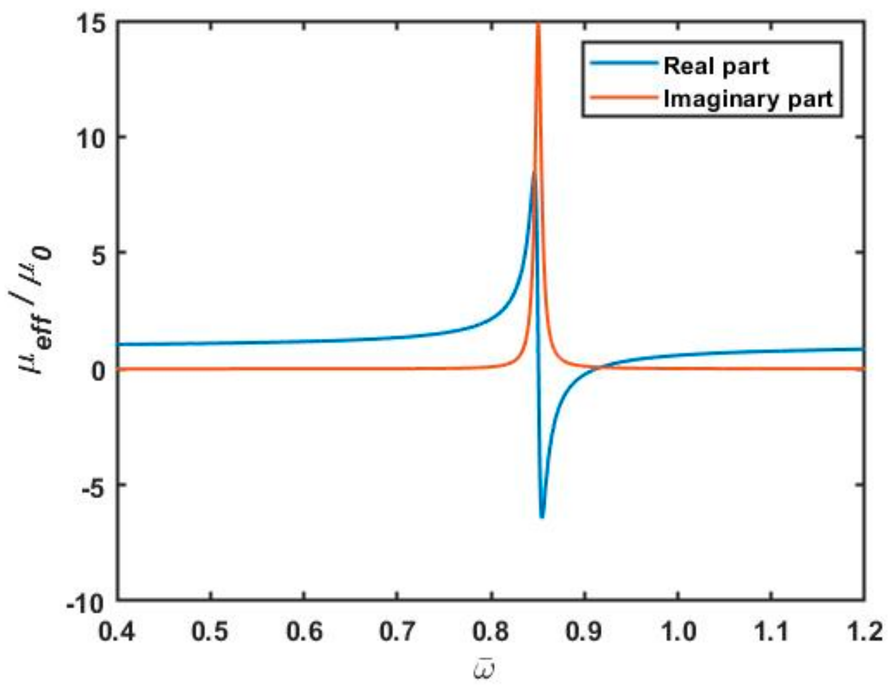
3. Dispersion in a Regularly Exampled MM
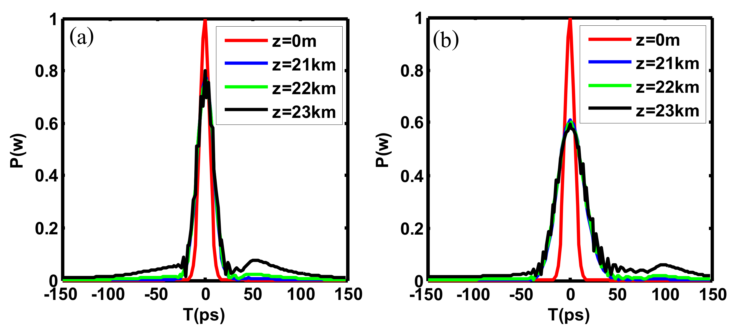
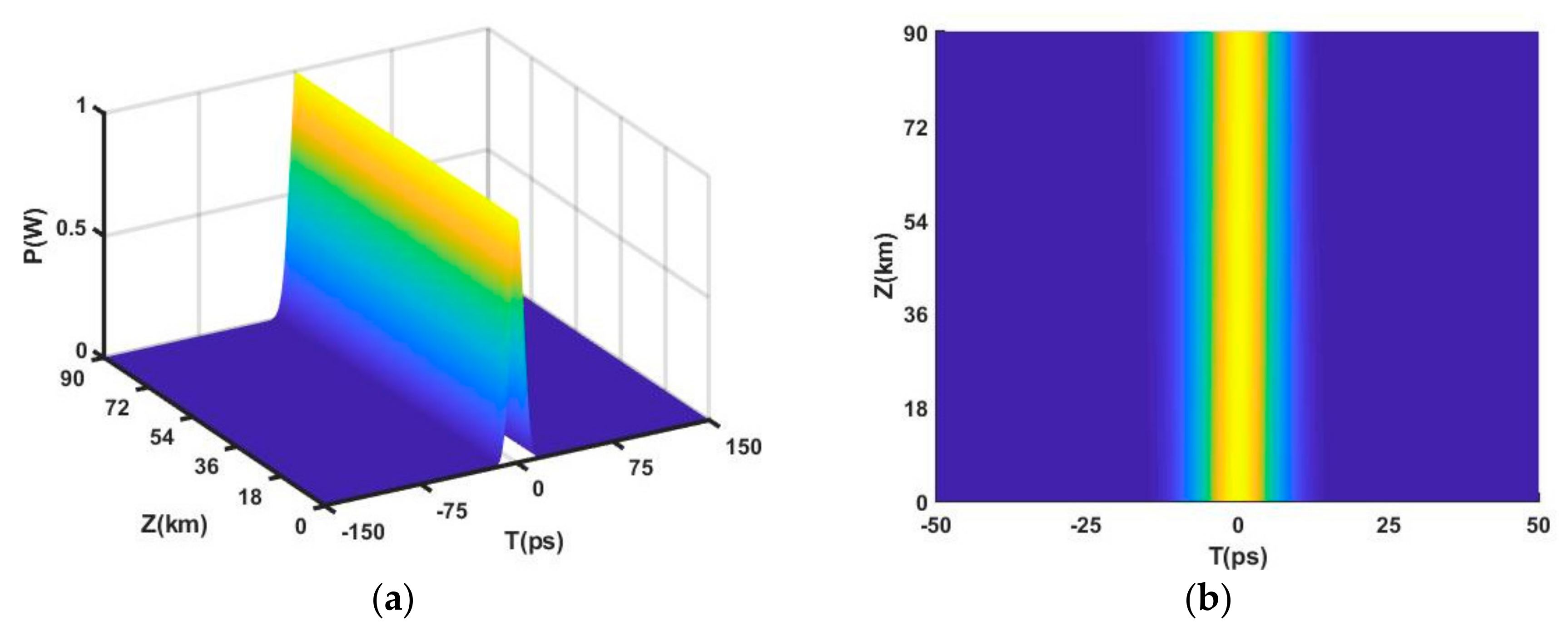
4. Light Pulse Propagation in the MM
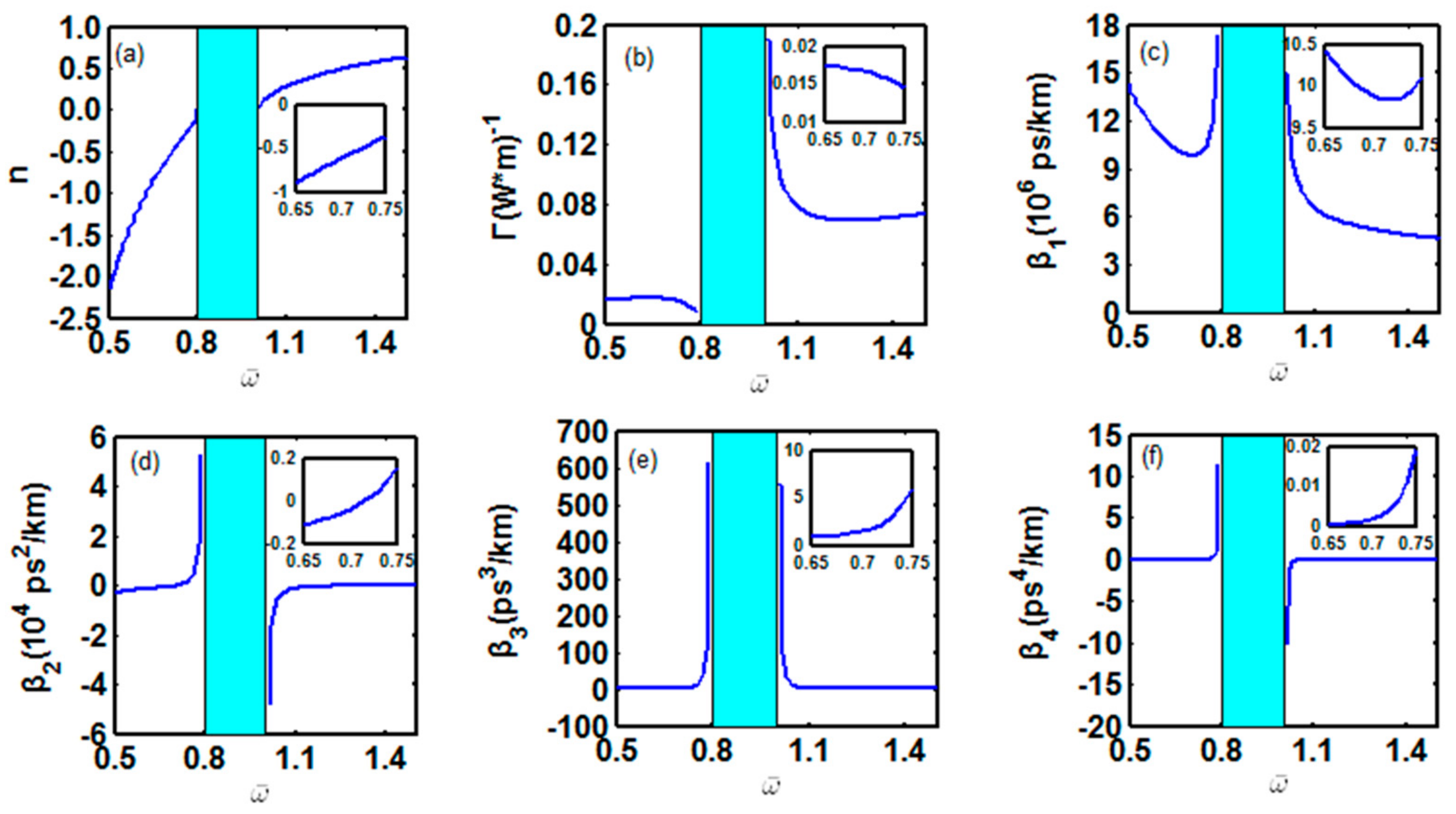
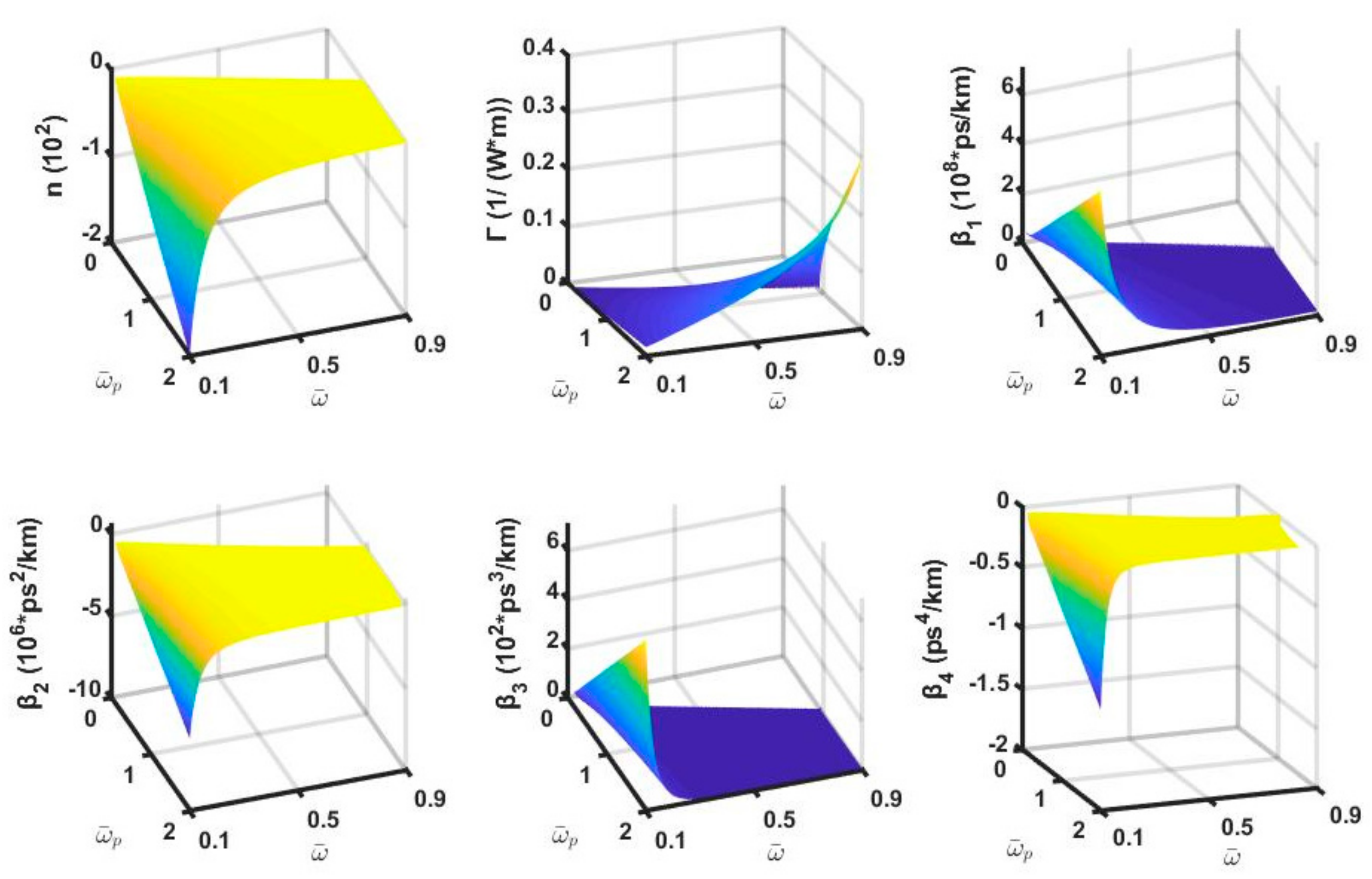
4.1. Impact of and
4.1.1. Impact of at
4.1.2. Impact of and when
4.1.3. Impact of and when
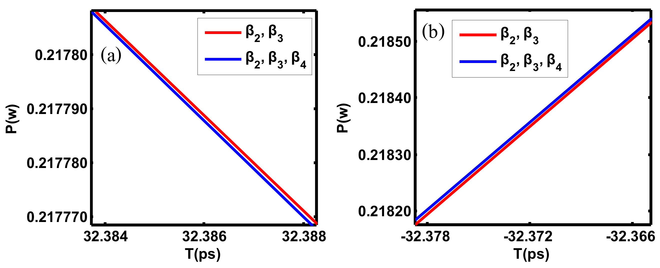
4.2. Impact of , , and
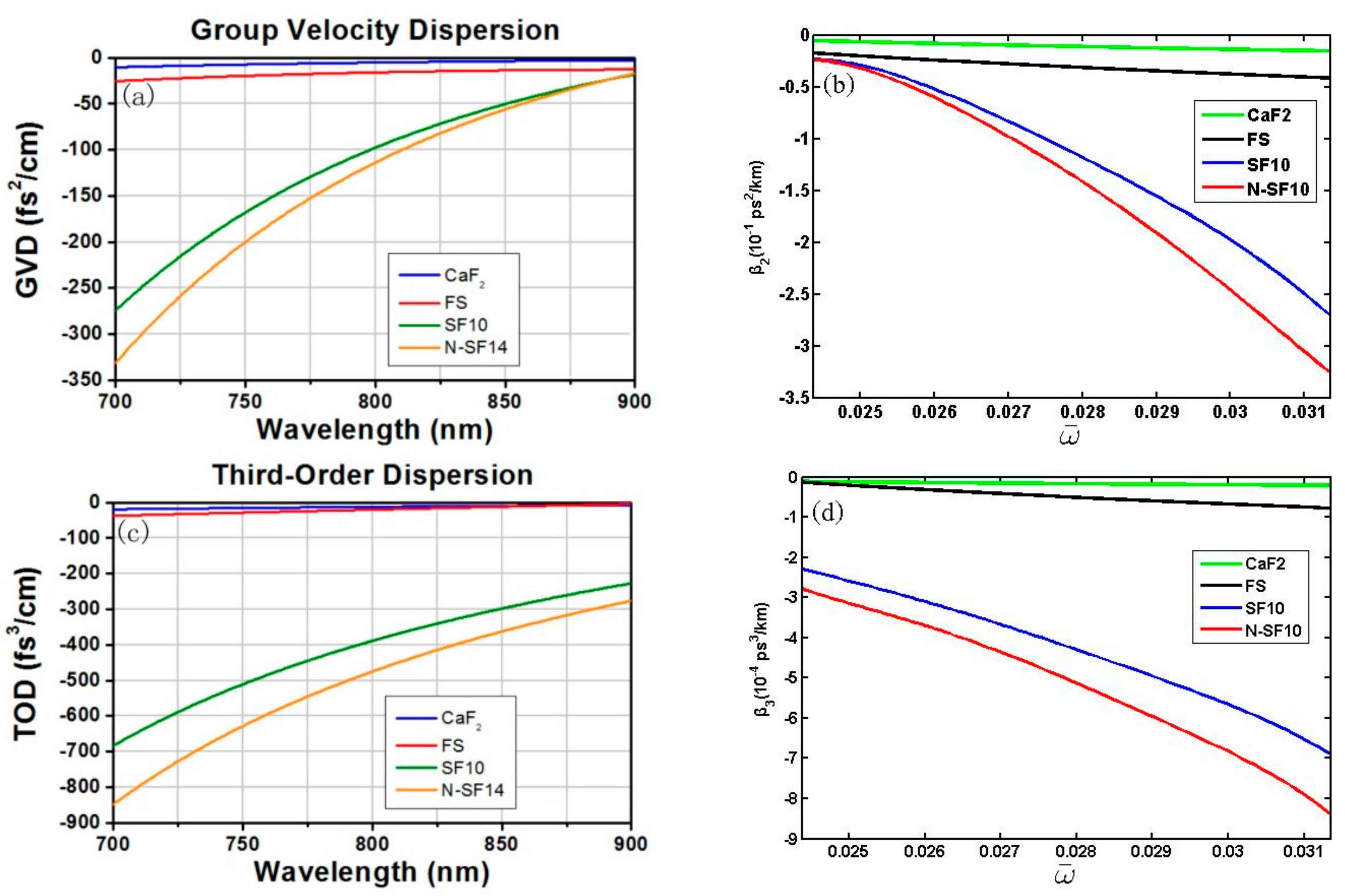
5. Dispersion Management in MMs
5.1. Design of the Optimal Dispersion
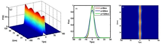
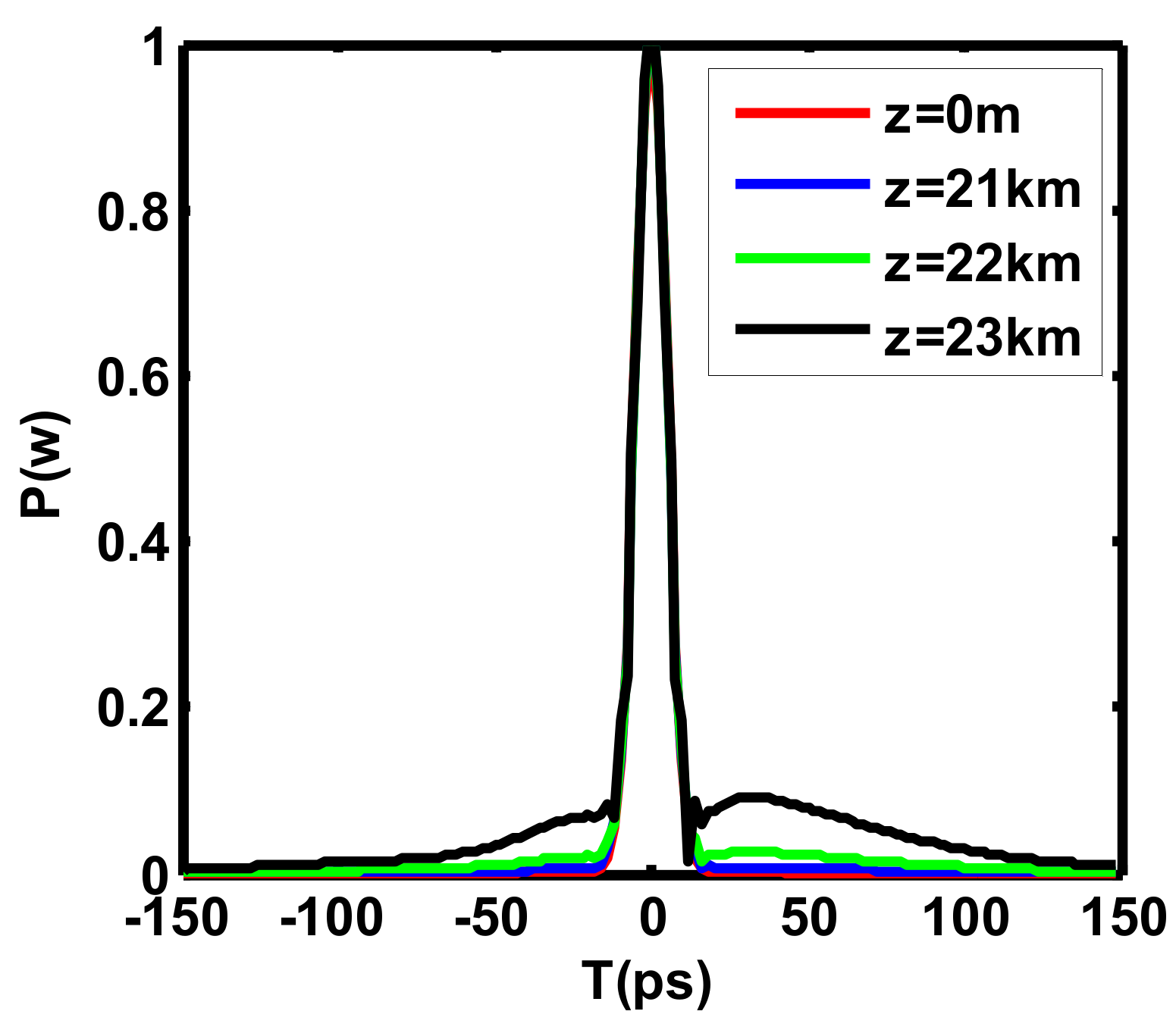
5.2. Dispersion Management
6. Conclusions
Author Contributions
Funding
Acknowledgments
Conflicts of Interest
Appendix A

| 0.8794293 | 1.277678 | 3.061317 | 0.039611 | 0.431031 | 0.0003325 | 631.1424 | 290.0022 |
| 0.8794294 | 1.277676 | 3.0613123 | 0.037757 | 0.43103 | 0.0003325 | 662.1362 | 290.0032 |
| 0.8794295 | 1.277674 | 3.0613075 | 0.035902 | 0.431028 | 0.0003325 | 696.3313 | 290.0042 |
| 0.8794296 | 1.277672 | 3.0613028 | 0.034048 | 0.431027 | 0.0003325 | 734.2507 | 290.0051 |
| 0.8794297 | 1.27767 | 3.061298 | 0.032194 | 0.431025 | 0.0003325 | 776.5378 | 290.0061 |
| 0.8794298 | 1.277668 | 3.0612933 | 0.03034 | 0.431024 | 0.0003325 | 823.9935 | 290.0071 |
| 0.8794299 | 1.277666 | 3.0612885 | 0.028486 | 0.431023 | 0.0003325 | 877.6269 | 290.0081 |
| 0.87943 | 1.277664 | 3.0612838 | 0.026632 | 0.431021 | 0.0003325 | 938.7285 | 290.009 |
| 0.8794301 | 1.277662 | 3.061279 | 0.024778 | 0.43102 | 0.0003325 | 1008.975 | 290.01 |
| 0.8794302 | 1.27766 | 3.0612743 | 0.022923 | 0.431018 | 0.0003325 | 1090.585 | 290.011 |
| 0.8794303 | 1.277658 | 3.0612695 | 0.021069 | 0.431017 | 0.0003325 | 1186.558 | 290.012 |
| 0.8794304 | 1.277656 | 3.0612648 | 0.019215 | 0.431015 | 0.0003325 | 1301.054 | 290.013 |
| 0.8794305 | 1.277654 | 3.06126 | 0.017361 | 0.431014 | 0.0003325 | 1440.005 | 290.0139 |
| 0.8794306 | 1.277652 | 3.0612553 | 0.015507 | 0.431012 | 0.0003325 | 1612.186 | 290.0149 |
| 0.8794307 | 1.27765 | 3.0612505 | 0.013653 | 0.431011 | 0.0003325 | 1831.133 | 290.0159 |
| 0.8794308 | 1.277648 | 3.0612458 | 0.011799 | 0.431009 | 0.0003325 | 2118.896 | 290.0169 |
| 0.8794309 | 1.277647 | 3.061241 | 0.009944 | 0.431008 | 0.0003325 | 2513.967 | 290.0178 |
| 0.879431 | 1.277645 | 3.0612363 | 0.00809 | 0.431007 | 0.0003325 | 3090.125 | 290.0188 |
| 0.8794311 | 1.277643 | 3.0612315 | 0.006236 | 0.431005 | 0.0003325 | 4008.897 | 290.0198 |
| 0.8794312 | 1.277641 | 3.0612268 | 0.004382 | 0.431004 | 0.0003325 | 5705.195 | 290.0208 |
| 0.8794313 | 1.277639 | 3.061222 | 0.002528 | 0.431002 | 0.0003325 | 9889.982 | 290.0218 |
| 0.8794314 | 1.277637 | 3.0612173 | 0.000674 | 0.431001 | 0.0003325 | 37111.35 | 290.0227 |
| 0.8794315 | 1.277635 | 3.0612125 | −0.00118 | 0.430999 | 0.0003325 | 21177.19 | 290.0237 |
| 0.8794316 | 1.277633 | 3.0612078 | −0.00303 | 0.430998 | 0.0003325 | 8238.099 | 290.0247 |
| 0.8794317 | 1.277631 | 3.061203 | −0.00489 | 0.430996 | 0.0003325 | 5113.68 | 290.0257 |
| 0.8794318 | 1.277629 | 3.0611983 | −0.00674 | 0.430995 | 0.0003325 | 3707.54 | 290.0267 |
| 0.8794319 | 1.277627 | 3.0611935 | −0.0086 | 0.430993 | 0.0003325 | 2907.928 | 290.0276 |
| 0.879432 | 1.277625 | 3.0611888 | −0.01045 | 0.430992 | 0.0003325 | 2392.034 | 290.0286 |
| 0.8794321 | 1.277623 | 3.061184 | −0.01231 | 0.430991 | 0.0003325 | 2031.607 | 290.0296 |
| 0.8794322 | 1.277621 | 3.0611793 | −0.01416 | 0.430989 | 0.0003325 | 1765.573 | 290.0306 |
| 0.8794323 | 1.277619 | 3.0611745 | −0.01601 | 0.430988 | 0.0003325 | 1561.145 | 290.0315 |
| 0.8794324 | 1.277617 | 3.0611698 | −0.01787 | 0.430986 | 0.0003325 | 1399.144 | 290.0325 |
| 0.8794325 | 1.277615 | 3.061165 | −0.01972 | 0.4309847 | 0.0003325 | 1267.604 | 290.0335 |
| 0.8794326 | 1.277613 | 3.0611603 | −0.02158 | 0.4309832 | 0.0003325 | 1158.672 | 290.0345 |
| 0.8794327 | 1.277611 | 3.0611555 | −0.02343 | 0.4309818 | 0.0003325 | 1066.98 | 290.0355 |
| 0.8794328 | 1.277609 | 3.0611508 | −0.02528 | 0.4309803 | 0.0003325 | 988.7366 | 290.0364 |
| 0.8794329 | 1.277607 | 3.061146 | −0.02714 | 0.4309789 | 0.0003325 | 921.1843 | 290.0374 |
| 0.879433 | 1.277605 | 3.0611413 | −0.02899 | 0.4309774 | 0.0003325 | 862.2722 | 290.0384 |
| 0.8794331 | 1.277603 | 3.0611366 | −0.03085 | 0.430976 | 0.0003325 | 810.4422 | 290.0394 |
| 0.8794332 | 1.277601 | 3.0611318 | −0.0327 | 0.4309745 | 0.0003325 | 764.4898 | 290.0403 |
| 0.8794333 | 1.277599 | 3.0611271 | −0.03456 | 0.4309731 | 0.0003325 | 723.4688 | 290.0413 |
| 0.8794334 | 1.277597 | 3.0611223 | −0.03641 | 0.4309716 | 0.0003325 | 686.6258 | 290.0423 |
| 0.8794335 | 1.277595 | 3.0611176 | −0.03826 | 0.4309702 | 0.0003325 | 653.3534 | 290.0433 |
| 0.8794336 | 1.277593 | 3.0611128 | −0.04012 | 0.4309687 | 0.0003325 | 623.1566 | 290.0443 |
| 0.8794337 | 1.277591 | 3.0611081 | −0.04197 | 0.4309673 | 0.0003325 | 595.6277 | 290.0452 |
| 0.8794338 | 1.277589 | 3.0611033 | −0.04383 | 0.4309658 | 0.0003325 | 570.4281 | 290.0462 |
| 0.8794339 | 1.277587 | 3.0610986 | −0.04568 | 0.4309643 | 0.0003325 | 547.2743 | 290.0472 |
| 0.879434 | 1.277585 | 3.0610938 | −0.04754 | 0.4309629 | 0.0003324 | 525.9267 | 290.0482 |
References
- Born, M.; Wolf, E. Princiiples of Optics; Cambridge University Press: Cambridge, UK, 1999; pp. 14–24. [Google Scholar]
- Shelby, R.A.; Smith, D.R.; Shultz, S.; Nemat-Nasser, S.C. Microwave transmission through a two-dimensional, isotropic, left-handed metamaterial. Appl. Phys. Lett. 2001, 78, 489–491. [Google Scholar] [CrossRef]
- Smith, D.R.; Padilla, W.J.; Vier, D.C.; Nemat-Nasser, S.C.; Schultz, S. Composite Medium with Simultaneously Negative Permeability and Permittivity. Phys. Rev. Lett. 2000, 84, 4184–4187. [Google Scholar] [CrossRef] [PubMed]
- Group Velocity Dispersion. Available online: https://www.thorlabs.us/images/TabImages/ AFS_prisms_GVD_G2-480.gif (accessed on 22 February 2018).
- Third Order Dispersion. Available online: https://www.thorlabs.us/images/TabImages/ AFS_prisms_TOD_G2-480.gif (accessed on 22 February 2018).
- Smith, D.R.; Pendry, J.B.; Wiltshire, M.C.K. Metamaterials and negative refractive index. Science 2004, 305, 788–792. [Google Scholar] [CrossRef] [PubMed]
- Engheta, R.; Ziolkowski, R.W. Metamaterials, Physics and Engineering Explorations; Wiley-IEEE: New York, NY, USA, 2006. [Google Scholar]
- Shalaev, V.M. Optical negative-index metamaterials. Nat. Photonics 2007, 1, 41–48. [Google Scholar] [CrossRef]
- Liu, Y.; Zhang, X. Metamaterials: A new frontier of science and technology. Chem. Soc. Rev. 2011, 40, 2494–2507. [Google Scholar] [CrossRef] [PubMed]
- Soukoulis, C.M.; Wegener, M. Past achievements and future challenges in the development of three-dimensional photonic metamaterials. Nat. Photonics 2011, 5, 523–530. [Google Scholar] [CrossRef]
- Zheludev, N.I.; Kivshar, Y.S. From metamaterials to metadevices. Nat. Mater. 2012, 11, 917–924. [Google Scholar] [CrossRef] [PubMed]
- Zheludev, N.I.; Plum, E. Reconfigurable nanomechanical photonic metamaterials. Nat. Nanotechnol. 2016, 11, 16–22. [Google Scholar] [CrossRef] [PubMed]
- Zheludev, N.I. Obtaining optical properties on demand. Science 2015, 348, 973–974. [Google Scholar] [CrossRef] [PubMed]
- Dastmalchi, B.; Tassin, P.; Koschny, T.; Soukoulis, C.M. Strong group-velocity dispersion compensation with phase-engineered sheet metamaterials. Phys. Rev. B 2014, 89, 115123. [Google Scholar] [CrossRef]
- Veselago, V.G. Electrodynamics of substances with simultaneously negative electrical and magnetic permeabilities. Sov. Phys. Usp. 1968, 10, 504–509. [Google Scholar] [CrossRef]
- Pendry, J.B.; Holden, A.J.; Stewart, W.J.; Youngs, I. Extremely Low Frequency Plasmons in Metallic Mesostructures. Phys. Rev. Lett. 1996, 76, 4773–4776. [Google Scholar] [CrossRef] [PubMed]
- Pendry, J.B.; Holden, A.J.; Robbins, D.J.; Stewart, W.J. Magnetism from conductors and enhanced nonlinear phenomena. IEEE Trans Microw. Theory Tech. 1999, 47, 2075–2084. [Google Scholar] [CrossRef]
- Shelby, R.A.; Smith, D.R.; Schultz, S. Experimental verification of a negative index of refraction. Science 2011, 292, 77–79. [Google Scholar] [CrossRef] [PubMed]
- Agrawal, G.P. Nonlinear Fiber Optics, 5th ed.; Academic Press: Cambridge, MA, USA, 2013. [Google Scholar]
- Liu, Y.; Xue, Y.L.; Yu, C. Modulation instability induced by cross-phase modulation in negative index materials with higher-order nonlinearity. Opt. Commun. 2015, 339, 66–73. [Google Scholar] [CrossRef]
- Shalaev, V.M.; Cai, W.; Chettiar, U.K.; Yuan, H.; Sarychev, A.K.; Drachev, V.P.; Kildishev, A.V. Nagative index of refraction in optical metamaterials. Opt. Lett. 2005, 30, 3356–3358. [Google Scholar] [CrossRef] [PubMed]
- Wen, S.; Wang, Y.; Su, W.; Xiang, Y.; Fu, X.; Fan, D. Modulation instability in nonlinear negative-index material. Phys. Rev. E 2006, 73, 036617. [Google Scholar] [CrossRef] [PubMed]
- Alù, A.; Salandrino, A. Negative effective permeability and left-handed materials at optical frequencies. Opt. Express 2006, 14, 1557–1567. [Google Scholar] [CrossRef] [PubMed]
- YXue, L.; Liu, W.; Gu, Y.; Zhang, Y. Light storage in a cylindrical waveguide with metamaterials. Opt. Laser Technol. 2015, 68, 28–35. [Google Scholar]
- Ordal, M.A.; Bell, R.J.; Alexander, R.W., Jr.; Long, L.L.; Querry, M.R. Optical properties of fourteen metals in the infrared and far infrared: Al, Co, Cu, Au, Fe, Pb, Mo, Ni, Pd, Pt, Ag, Ti, V, and W. Appl. Opt. 1985, 24, 4493–4499. [Google Scholar] [CrossRef] [PubMed]
- Ordal, M.A.; Long, L.L.; Bell, R.J.; Bell, S.E.; Bell, R.R.; Alexander, R.W.; Ward, C.A. Optical properties of the metals Al, Co, Cu, Au, Fe, Pb, Ni, Pd, Pt, Ag, Ti, and W in the infrared and far infrared. Appl. Opt. 1983, 22, 1099–1119. [Google Scholar] [CrossRef] [PubMed]


| 0.70680 | −1.2589 | 2.0676 | 19.86 | 60.46 |
| 0.70675 | −2.6715 | 2.0675 | 9.36 | 60.53 |
| 0.70690 | 1.5715 | 2.0726 | 15.91 | 60.31 |
| 0.70695 | 2.9894 | 2.0752 | 8.36 | 60.24 |
| 0.706587 | −7.2648 | 2.0569 | 0.0037 | 3.44 | 60.77 |
| 0.70710 | 7.2532 | 2.0828 | 0.0037 | 3.45 | 60.02 |
| 0.8794313 | 1.277639 | 3.061222 | 0.002528 | 0.431002 | 0.0003325 | 9889.982 | 290.0218 |
| 0.8794314 | 1.277637 | 3.0612173 | 0.000674 | 0.431001 | 0.0003325 | 37111.35 | 290.0227 |
| 0.8794315 | 1.277635 | 3.0612125 | −0.00118 | 0.430999 | 0.0003325 | 21177.19 | 290.0237 |
| Metamaterial | ||||||
|---|---|---|---|---|---|---|
| MM1 | 0.88 | 0.941095 | 1.184911 | 0.330214 | 21.10 | 378.56 |
| MM2 | 0.88 | 0.941240 | −1.183498 | 0.327182 | 21.12 | 382.03 |
© 2018 by the authors. Licensee MDPI, Basel, Switzerland. This article is an open access article distributed under the terms and conditions of the Creative Commons Attribution (CC BY) license (http://creativecommons.org/licenses/by/4.0/).
Share and Cite
Xu, Z.G.; Xue, Y.L.; Huang, Z. Dependence of Dispersion on Metamaterial Structural Parameters and Dispersion Management. Appl. Sci. 2018, 8, 1057. https://doi.org/10.3390/app8071057
Xu ZG, Xue YL, Huang Z. Dependence of Dispersion on Metamaterial Structural Parameters and Dispersion Management. Applied Sciences. 2018; 8(7):1057. https://doi.org/10.3390/app8071057
Chicago/Turabian StyleXu, Zheng Guo, Yan Ling Xue, and Zhihao Huang. 2018. "Dependence of Dispersion on Metamaterial Structural Parameters and Dispersion Management" Applied Sciences 8, no. 7: 1057. https://doi.org/10.3390/app8071057
APA StyleXu, Z. G., Xue, Y. L., & Huang, Z. (2018). Dependence of Dispersion on Metamaterial Structural Parameters and Dispersion Management. Applied Sciences, 8(7), 1057. https://doi.org/10.3390/app8071057