Article

Output Power Smoothing Control for a Wind Farm Based on the Allocation of Wind Turbines

1
College of Energy and Electrical Engineering, Hohai University, Nanjing 211100, China
2
State Grid Nanjing Power Supply Company, State Grid Jiangsu Electric Power CO. LTD., Nanjing 210008, China
*
Author to whom correspondence should be addressed.
Appl. Sci. 2018, 8(6), 980; https://doi.org/10.3390/app8060980
Submission received: 18 May 2018 / Revised: 5 June 2018 / Accepted: 13 June 2018 / Published: 15 June 2018
(This article belongs to the Special Issue Large Grid-Connected Wind Turbines)

Abstract

:
This paper presents a new output power smoothing control strategy for a wind farm based on the allocation of wind turbines. The wind turbines in the wind farm are divided into control wind turbines (CWT) and power wind turbines (PWT), separately. The PWTs are expected to output as much power as possible and a maximum power point tracking (MPPT) control strategy combining the rotor inertia based power smoothing method is adopted. The CWTs are in charge of the output power smoothing for the whole wind farm by giving the calculated appropriate power. The battery energy storage system (BESS) with small capacity is installed to be the support and its charge and discharge times are greatly reduced comparing with the traditional ESSs based power smoothing strategies. The simulation model of the permanent magnet synchronous generators (PMSG) based wind farm by considering the wake effect is built in Matlab/Simulink to test the proposed power smoothing method. Three different working modes of the wind farm are given in the simulation and the simulation results verify the effectiveness of the proposed power smoothing control strategy.

1. Introduction

Wind energy is the most mature and promising renewable energy source in the world at present. The doubly-fed induction generator (DFIG) based and direct-drive permanent magnet synchronous generator (PMSG) based systems are the most popular wind energy conversion systems (WECS), which are widely used in wind farms [1]. Though both of the two WECSs have their own advantages and disadvantages, the direct-drive PMSG based WECSs are preferred in high power applications owing to the simple structure, high efficiency, and high reliability due to the absence of gearboxes [1,2,3]. However, due to the stochastic nature of wind, the output power of the wind farm is fluctuating, which brings negative influences to the stability and economy of the grid operation. Specifically, the problems caused by the wind power fluctuations are listed as: frequency deviation, voltage flicker, low power quality, and harm to sensitive loads [3,4,5]. To solve these problems, several methods are proposed to smooth the output power of the wind farm, which can be basically divided into two major categories: direct power control and indirect power control.
The direct power control usually depends on using the wind turbine (WT) itself without energy storage devices, such as through the DC bus voltage control, rotor inertia control, and the pitch angle control [3,6,7,8,9,10,11]. However, the DC bus voltage control may cause the excessive voltage ripple, thus affecting normal operation of the WECS [5]. For the rotor inertia control, the rotor speed is always controlled to exceed the rated value to store the kinetic energy. According to the research [5], the efficiency of the kinetic energy control relying on the generator inertia is close to the maximum power point tracking (MPPT) control. The trade-off between the maximum power tracking and power smoothing is explored through the optimal control of WTs based on the rotating kinetic energy reserves in references [7,8]. The pitch angle control has to operate at a fast rate, thus mechanical stress accrues in the wind turbine blade. Besides, the direct power control methods always focus on the output power smoothing of a single WT, which may lead to the poor effect for the entire wind farm. In addition, all the smoothing capability of the direct power control method is constrained by the rated power of the WTs.
The indirect power control is realized by using energy storage systems (ESS), such as the battery, the supercapacitor, the superconductor magnetic energy storage (SMES), the flywheel, and so on [12,13,14,15,16,17,18,19]. But all existing ESSs have certain problems in practical application. The charge-discharge cycles of the battery are limited, although many types of batteries are quite mature at present [12,13]. The supercapacitor has the much longer life of charge-discharge processing than that of batteries, but it cost too much to be used on a large scale [14]. SMES is a large superconducting coil that can store electric energy in the magnetic field produced by the flow of a DC current through it. The effectiveness of the SMES is demonstrated by many studies, but it is still too costly [15,16]. The flywheel ESS utilizes the kinetic energy of a rotating disc, which depends on the square of the rotational speed. It has the advantages of long cycling life, large energy storage capacity, and high reliability [17,18]. However, the drawbacks of immature technology, large size, and high standing losses cannot be ignored in practical use at present. Then hybrid ESSs for smoothing out wind power fluctuations are proposed in literatures to overcome the disadvantages of the single ESS, but the control strategies are more complicated [19].
As above, all the existing power smoothing control strategies have both advantages and disadvantages, which result in difficulties for practical application. In order to solve such problems, a power smoothing method based on the allocation of the wind turbines and the rotor inertia is proposed in this paper, which is quite different from the above-mentioned power smoothing methods. In this paper, the direct-drive PMSG based WECS is chosen in the wind farm. The WTs of the wind farm are divided into two classes: control wind turbines (CWT) and power wind turbines (PWT). The PWTs are expected to output as much power as possible and then the MPPT control strategies are adopted by combing the power smoothing strategy using rotor inertia. The increment of wind power can be stored in the generator as a form of kinetic energy and released when the wind power decreases. The CWTs are in charge of the output power smoothing for the entire wind farm by giving the appropriate power according to the output power need of the wind farm. The battery energy storage system (BESS) with small capacity is installed as the back support of the CWTs to satisfy the high power demanding of the grid. The simulation model of the wind farm based on the proposed control strategies is built in Matlab/Simulink and the efficiency of the proposed strategy is verified by the simulation results.

2. Wind Energy Conversion System Description

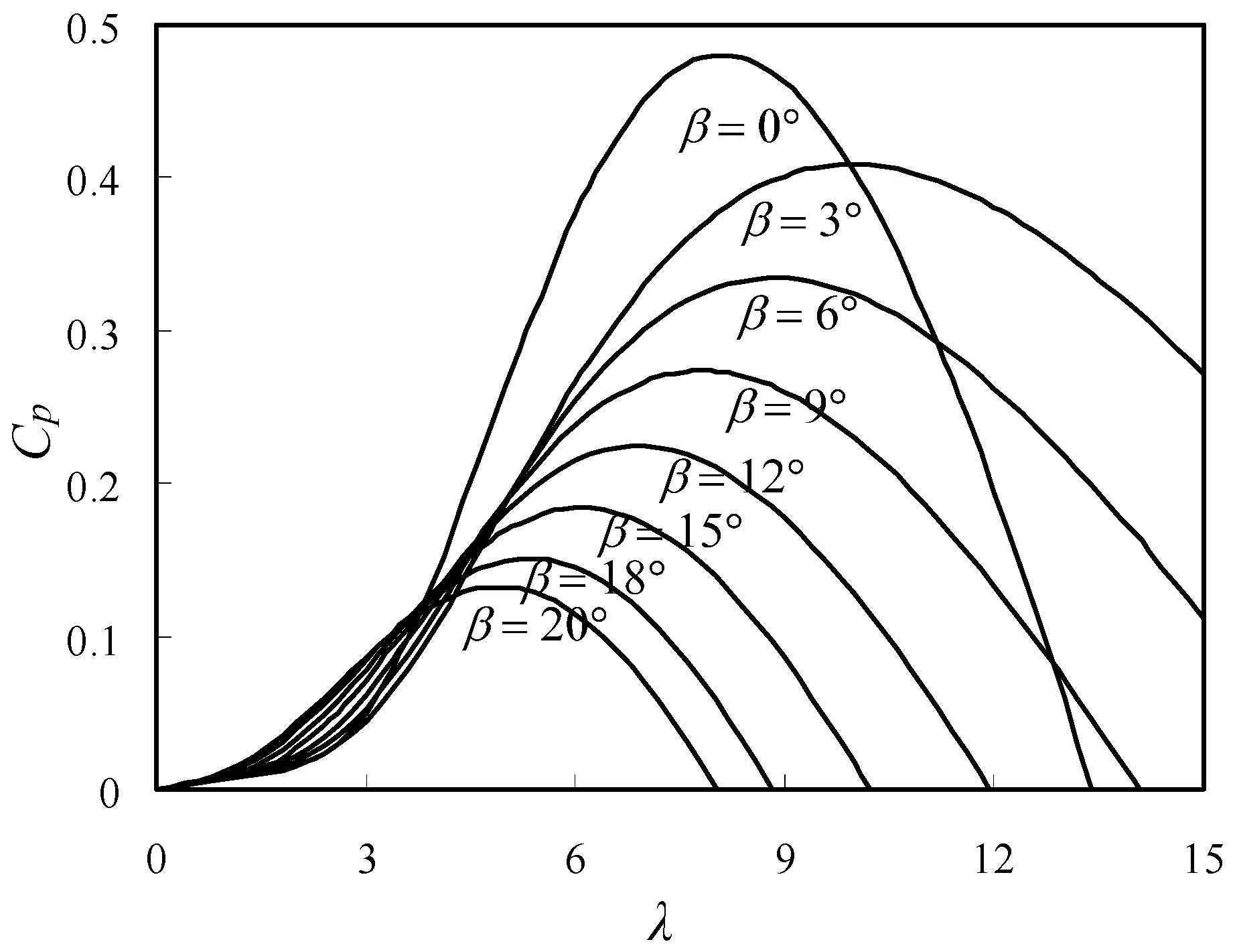
2.1. Wind Turbine Model

The mechanical power generated by a wind turbine is [20]:
P w = ρ π R 2 C p ( λ , β ) v 3 / 2 ,
where ρ is air density, R is turbine blade radius, v is wind speed and Cp is power coefficient which is a function of the tip speed ratio (TSR) λ and blade pitch angle β. λ is defined as:
λ = ω o R / v ,
where ωo indicates the rotational speed in rad/s.
The output torque of the wind turbine is:
T = ρ π R 3 C p ( λ , β ) v 2 / 2 λ
According to Equation (2), the rotor speed can be adjusted to keep λ at the optimum value λopt and then maximize the power coefficient as Cpmax. The wind turbine aerodynamic efficiency Cp (λ, β) is given by the following Equation [21]:
{ C p ( λ , β ) = 0.5176 ( 116 α 0.4 β 5 ) e 21 / α + 0.0068 λ 1 α = 1 λ + 0.08 β 0.035 β 3 + 1
where α is the intermediate variable to obtain the Cp by using λ and β. The curves of the power coefficient Cp and the TSR λ with different blade pitch angles are shown in Figure 1. It can be seen that the maximum power coefficient is decreasing by increasing the pitch angle. Therefore, the output power of the wind turbine can be limited to the rated value through the variable pitch angle control.
According to (1) and (2), the maximum power output of the wind turbine is obtained as:
P w o p t = ρ π R 5 C p max ω 3 / 2 λ o p t 3 = k o p t ω 3 .
Then the optimum torque is expressed as
T o p t = ρ π R 5 C p max ω 2 / 2 λ o p t 3 = k o p t ω 2 ,
where kopt is the coefficient associated with the wind turbine characteristics.

2.2. PMSG Model

The voltage equations of the PMSG in decoupled dq-axes rotating reference frame are expressed as [21]:
{ u d s = R s i d s + p ψ d s ω e ψ q s u q s = R s i q s + p ψ q s + ω e ψ d s ,
where uds, uqs are the stator winding voltages in dq-axes. ids, iqs are the stator winding currents in dq-axes. ψds, ψqs are the stator winding magnet fluxes in dq-axes. ωe is the rotor speed, Rs is the resistance of the stator windings.
The magnet flux equations of PMSG in dq-axes rotating reference frame are expressed as
{ ψ d s = L d i d s + ψ f ψ q s = L q i q s ,
where ψf is the permanent magnet flux. Ld, Lq are the stator winding inductances in dq-axes.
The electromagnetic torque of PMSG is given as:
T e = n p [ ψ f i q s + ( L d L q ) i d s i q s ] ,
where np is the pole pairs of the PMSG.
The motion equation of the PMSG is expressed as:
T L F ω T e = J d ω d t ,
where TL is the input load torque, F is friction coefficient, J is the moment of inertia, ω is the mechanical rotor speed.

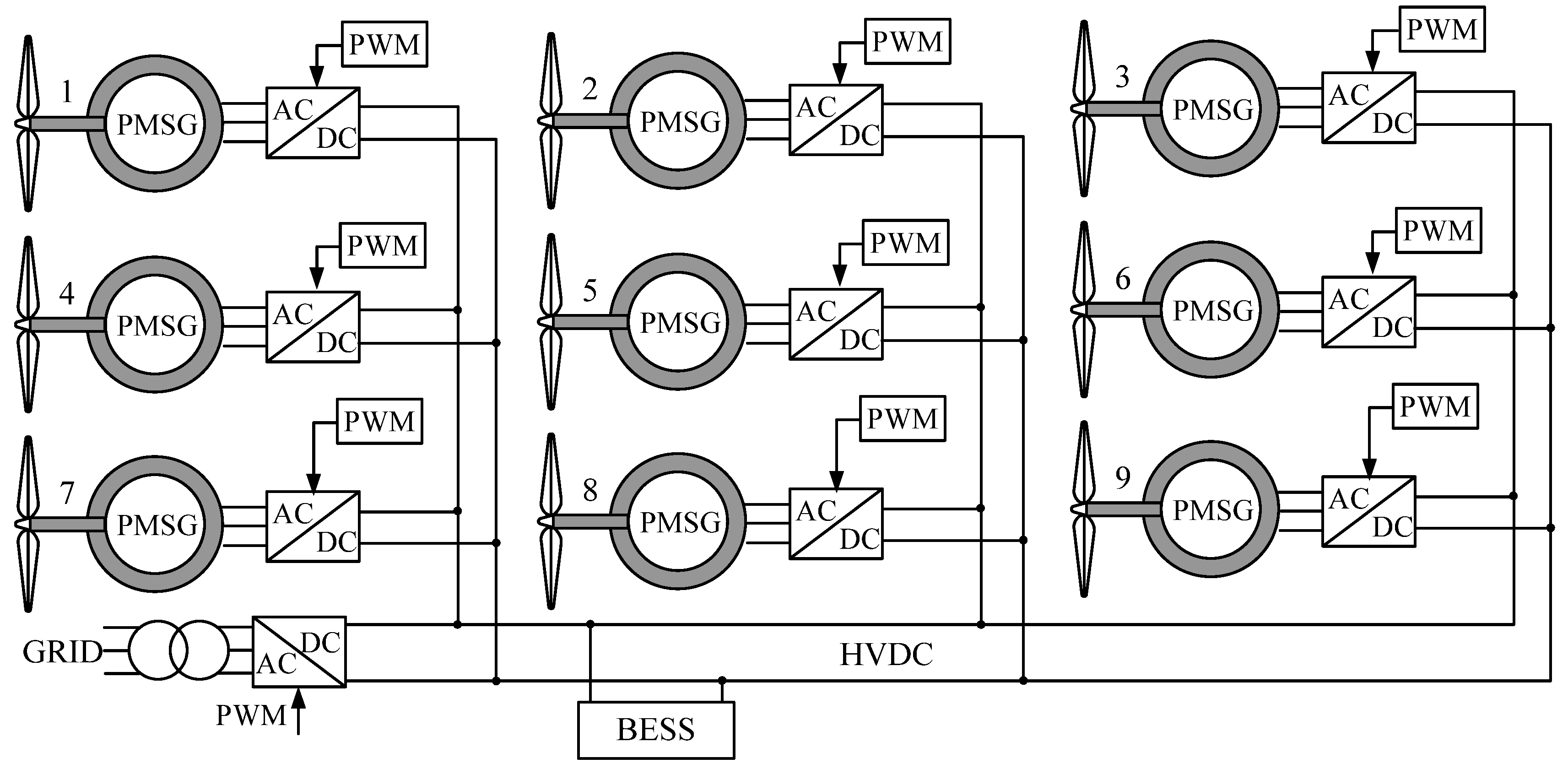
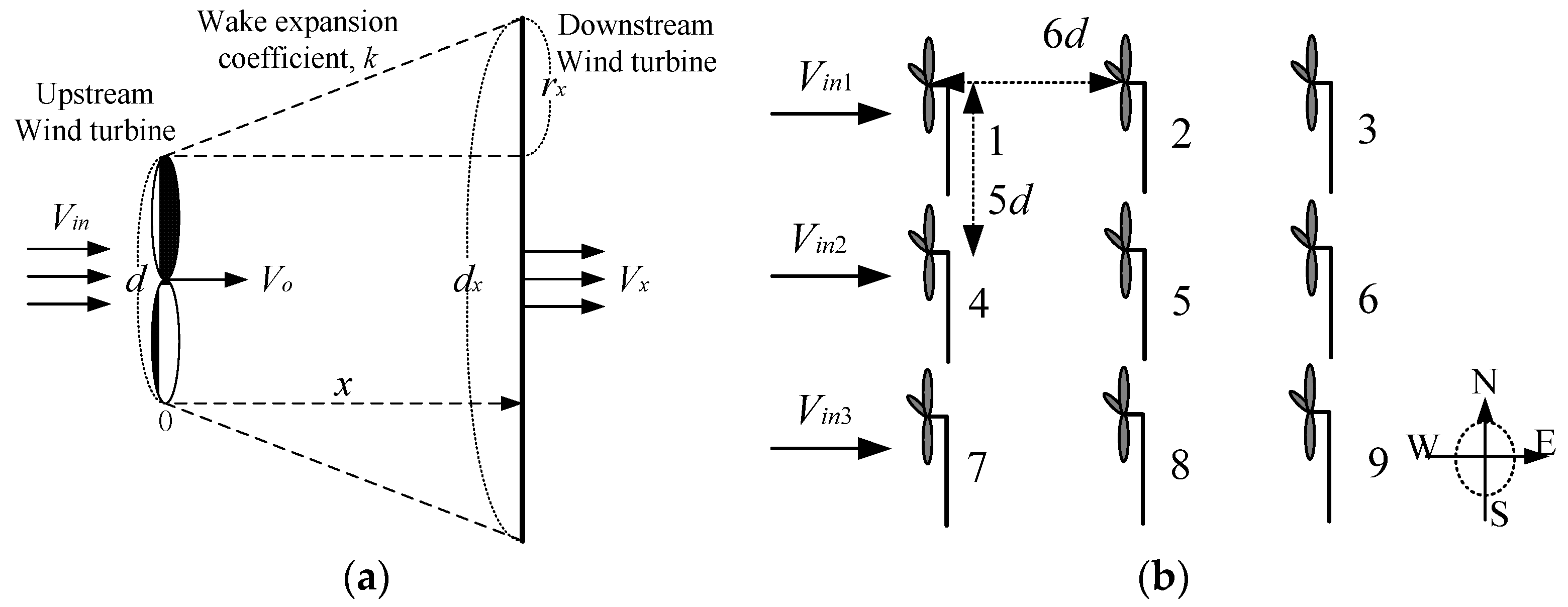
2.3. Configuration of the Wind Farm

The layout of the wind farm model built in this paper is shown in Figure 2. The wind farm comprised nine PMSG based wind turbines arranged in three rows and three columns. The traditional grid-connection mode of the PMSG based WECS, which was composed of the PMSG and the back-to-back converter, was not adopted in the wind farm model of this paper. Here, the alternating voltage generated by the PMSG was converted into the direct voltage by the generator-side converter and then connected to the DC bus. Apart from the high power transfer capability and cost-effectiveness in a longer transmission system, HVDC is also considered as an environmentally friendly technology owing to its low corona losses and ozone generation rates [22]. Thus, the power is delivered and converged in the cables through the mode of high voltage direct current (HVDC) in this paper. Afterwards, the direct current power was inverted to the alternating current power and transmitted into the grid through the shared grid-connected inverter. The number of grid-connected inverters was decreased, as compared to the traditional grid-connection mode of the PMSG based WECS and then the cost was reduced. The nine wind turbines were divided into three groups according to the topographic location, turbines 1–3 is group one, turbines 4–6 is group two and turbines 7–9 is group three. The BESS was connected to the HVDC DC link to be the support of the CWTs as shown in Figure 2.

2.4. Wake Effect Model of the Wind Farm

In a wind farm, the wind speed of downstream wind turbines was affected by the upstream turbines due to the air flow and the power loss that happened is called wake effect. The Jensen wake model is used commonly in the wind farm simulation due to its simplicity and validity for the far field [23,24]. In this paper, the Jensen model was adopted to generate the wind speed of the downstream WTs as shown in Figure 3a. The basic Jensen wake effect model is shown in Figure 3 and the wind speed of downstream WTs is expressed as [23]:
V x = V i n [ 1 ( 1 1 C t ) ( d d x ) 2 ] ,
where Vx is the downstream wind speed, Vin is the free stream wind speed, d is the diameter of the WT rotor, x is the distance between the WTs, k is the wake expansion coefficient which represents the effects of atmospheric stability, and dx = d + 2kx. In general, k is set as 0.075 for onshore wind farms and 0.05 for offshore wind farms. In this paper, k was set as 0.075. Ct is the thrust coefficient which is usually given by the wind turbine manufacturer or can be calculated according to the simulation software by giving the required data. In this paper, Ct was set as 0.8 when the wind speed was between 3 and 12 m/s by consulting the Vestas V80 type [24].
The leeside speed can be obtained according to Equation (11) by assuming the x is zero as:
V o = V i n 1 C t
In practical wind farms, free wind speed can be affected by both obstacles and other WTs around which is called the wind shade effect [23]. Then the Equation (11) can be modified as by considering this effect:
V x = V i n [ 1 ( 1 1 C t ) ( d d x ) 2 ( A s A ) ] ,
where As is the shade area caused by the other upstream WTs, and A is area of the downstream WT. Most wind farms consist of a large number of WTs, thus the cumulative shade effect of each WT should be considered. Thus, the Equation (13) is modified as
V x = V i n [ 1 i n ( 1 1 C t ) ( d d x i ) 2 ( A s i A ) ] :
where n is the number of influencing upstream WTs, Asi is the shade area caused by upstream WT i. The method for calculating the shade area is introduced in [24].
The height of WTs and the wind direction are also important factors in the consideration of wake effect and the details can be seen in [23]. In this paper, the height of the nine WTs was the same and the wind direction was set as from west to east. The layout of the wind turbines was chosen according to the industry standards, as shown in Figure 3b, while the distance between the WTs in the west-east direction was 6d and the distance between the WTs in the north-south direction was 5d [24]. The WTs of the second row was affected by the first row WTs and the wind speed of the third row was affected by both the first and second row WTs. The wind speed deficit of WTs at the second row and third row can be calculated by the equations in [25,26]. The Jensen’s wake effect model adopted in this paper was used to generate the wind speed for all WTs in the wind farm by giving the nature stochastic wind speed to the first row WTs.

3. Power Smoothing Control Strategy

3.1. Power Allocation of the PWTs, CWTs and the BESS

The wind turbines of the wind farm were divided into CWTs and PWTs with different control targets in the proposed power smoothing control strategy of this paper. The PWTs adopted the MPPT control strategies by combing the rotor inertia based power smoothing strategy. The CWTs were in charge of the output power smoothing for the wind farm by giving the appropriate power according to the output power need and the right calculations. The BESS with small capacity was configured as the back support of the CWTs to satisfy the high power demanding of the grid. This paper focuses on the wind turbine allocation based power smoothing control strategy itself and then the quantity configuration of the CWTs and PWTs was not discussed due to the limited space. Here, in the wind farm shown in Figure 2, the wind turbines 1–6 were chosen to be the PWTs while the turbines 7–9 were the CWTs.
The power allocation method of the WTs and the BESS for the proposed power smoothing control strategy is shown in Figure 4. All the WTs of the wind farm were controlled to output the maximum power if the grid demand power of the wind farm Pgiven exceeded the maximum capability of the WTs P∑_max. At this time, the demand power cannot be reached and the BESS will work in the discharging state as shown in the gray box of Figure 4. The discharge power of the BESS was obtained by Pgiven subtracting the output power of the all WTs. When the maximum output power of the wind farm was more than the demand power, the judgment will be continued.
Then when the demand power was more than the sum of the maximum output power of the PWTs and the minimum output power of the CWTs, the BESS will be on the rest as shown in the yellow box of Figure 4 and the PWTs will be controlled to output the maximum power. The reference power of the CWTs can be obtained by Pgiven subtracting the output power of PWTs. Otherwise, the CWTs were controlled to output the minimum power and the process will continue by comparing the state of charge (SOC) of the BESS with the specified maximum value SOCmax.
The BESS was on the rest when the real-time SOC exceeded the SOCmax, as shown in the yellow box of Figure 4. At this time the control target of the PWTs should be changed as the reference power of the PWTs were given by Pgiven subtracting the minimum output power of CWTs. Otherwise, the BESS will be in the charging state, as shown in the blue box of Figure 4 and the main judgment process will continue. The calculated charging power should be compared with the maximum charging power capability of the BESS Pess_max.
If the calculated charging power was beyond Pess_max, the reference charging power was set to the value Pess_max. Then the reference power of PWTs will be obtained according to Pgiven, Pess and Pcontrol_min. If the calculated charging power was less than Pess_max, the PWTs will be controlled to output the maximum power and the extra power was stored in the BESS. The red digital markers (1)–(3) in Figure 4 are referring to the general power allocation of CWTs and PWTs. The detailed reference power for each CWT and PWT can be obtained according to the wind speed relationship between each WT. Though the Jensen wake effect model is widely used in engineering due to its simplicity, it is not accurate enough in prediction over short-term period, as well as for wind farm application. Thus, the wind speed of each WT needed in the control process was not calculated according to the wake effect model. It can be achieved through the anemoscope simply. Alternatively, short-term wind speed forecasting can be utilized to get the wind speed, which will be studied by authors next.
In Figure 4, Ppower_max and Pcontrol_max indicate the maximum output power of the power wind turbines and control wind turbines, respectively. The maximum output power was based on the equation P w = ρ π R 2 C p ( λ , β ) v 3 / 2 while Cp is the maximum value (0.48 in the manuscript). In the practical application, the efficiency of the wind turbine η should be considered and then P p o w e r _ max = η ρ π R 2 C p max v p o w e r 3 / 2 , P c o n t r o l _ max = η ρ π R 2 C p max v c o n t r o l 3 / 2 . In the simulation, many losses, such as iron loss and mechanical loss, are not considered. Then the efficiency of the wind turbines were relatively high and the efficiency was set as 0.95 in this paper. The minimum output power of CWTs Pcontrol_min can be changed according to the wind speed condition and wind farm or grid demand.

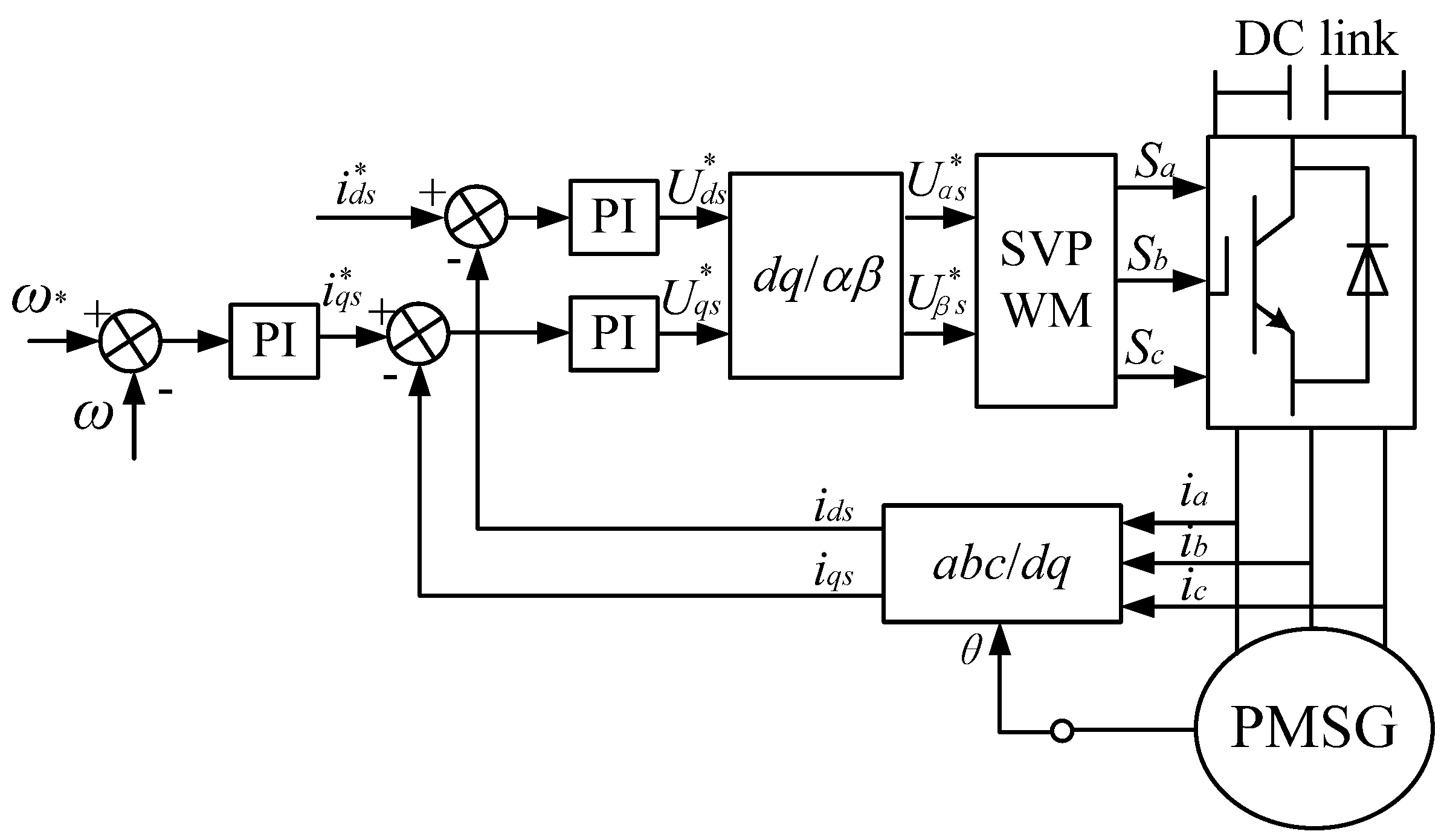
3.2. Control Strategy for the PWTs

The control purpose of the PWTs was to output the relatively smoother maximum power. Then the power given MPPT control with the rotor inertia based power smoothing control was adopted. The rotor inertia based power smoothing method can reduce the rotor torque ripple and then reduce the mechanical stress of the generator. The idea of the rotor inertia control was to use the kinetic energy in the rotor inertia of the wind turbine to smooth the output power of the system, especially when the inertia was significant, it can be regarded as an energy storage device [27]. The kinetic energy of the wind turbine will increase due to the acceleration of the rotor speed when the wind speed increases fast. Otherwise, the kinetic energy will release due to the decline of the rotor speed when the wind speed decreases.
The average value of the maximum wind power in Equation (5) can be calculated as [5]:
P a v g = 1 T t T t P w o p t d t ,
where t is the real time and T is the sampling period. The power difference of the optimum value and the average value determines the storing and restoring power in inertia of the wind turbine. Then the integral of the difference power is the redundant kinetic energy. The kinetic energy of the wind turbine can is calculated as [5]:
E = 1 2 J ω 2 .
Thus, the reference kinetic energy can be given as:
E = 1 2 J ω 2 + ( P w o p t P a v g ) .
Then the reference rotor speed is
ω = 2 E / J .
Finally, the output power smoothing by using the kinetic energy can be realized by giving the reference wind turbine rotor speed shown in Equation (18). The power smoothing effect relies on parameters, such as the wind turbine rotor inertia J and the sampling period T. The greater the rotor inertia is, the better the smoothing effect is. However, the big rotor inertia will bring a lot of difficulties for the system control, such as reducing the control response speed.
As shown in Equation (17), the traditional kinetic energy control compares the optimum power and the average value of the optimum power in a period to obtain the needed smoothing power. The principle of taking an average is simple, but the sampling period and system sampling precision are very important in the process. The low-pass filter is used widely in the wind power smoothing filed combing with the energy storage devices. In this paper, the low-pass filter is used to replace the averaging step to simplify the control process and then the Equation (17) will be changed as:
E = 1 2 J ω 2 + ( P w o p t P f i l t e r ) ,
where Pfilter is the maximum power after low-pass filtering. The rotor inertial power smoothing based MPPT control by adopting the low-pass filter is shown in Figure 5. The cut-off frequency of the low-pass filter is set according to the power smoothing demand of the grid. The lower the cut-off frequency is, the smoother the output power is. Ts is the sampling time of the kinetic energy.
After calculating the reference rotor speed ω*, the actual speed ω is compared with ω* and the difference was imported to a Proportional Integral (PI) controller. For realizing the vector control of the PMSG, the real three phase currents (ia, ib, ic) were transformed into direct axis (d-axis) current ids and quadrature axis (q-axis) current iqs through the combination of the Clark transformation and Park transformation (abc/dq) using the rotor position θ. The reference q-axis current i*qs was obtained from the speed PI loop. id = 0 control was adopted widely due to its simplicity and practicality [28]. Thus, the reference d-axis current i*ds was set to zero to simplify the control. The reference current was compared with the actual current and the difference is input to the current PI loop, as shown in Figure 6. Then the reference d-axis voltage U*ds and q-axis voltage U*qs were achieved from the current PI loops. The reference α-axis voltage U*αs and β-axis voltage U*βs in the two-phase static frame were obtained according to the inverse Park transformation. The space vector pulse width modulation (SVPWM) method [29] was adopted here to generate the PWM signal of the generator-side converter (Sa, Sb, Sc). The complete control diagram of the PWTs is presented in Figure 6.

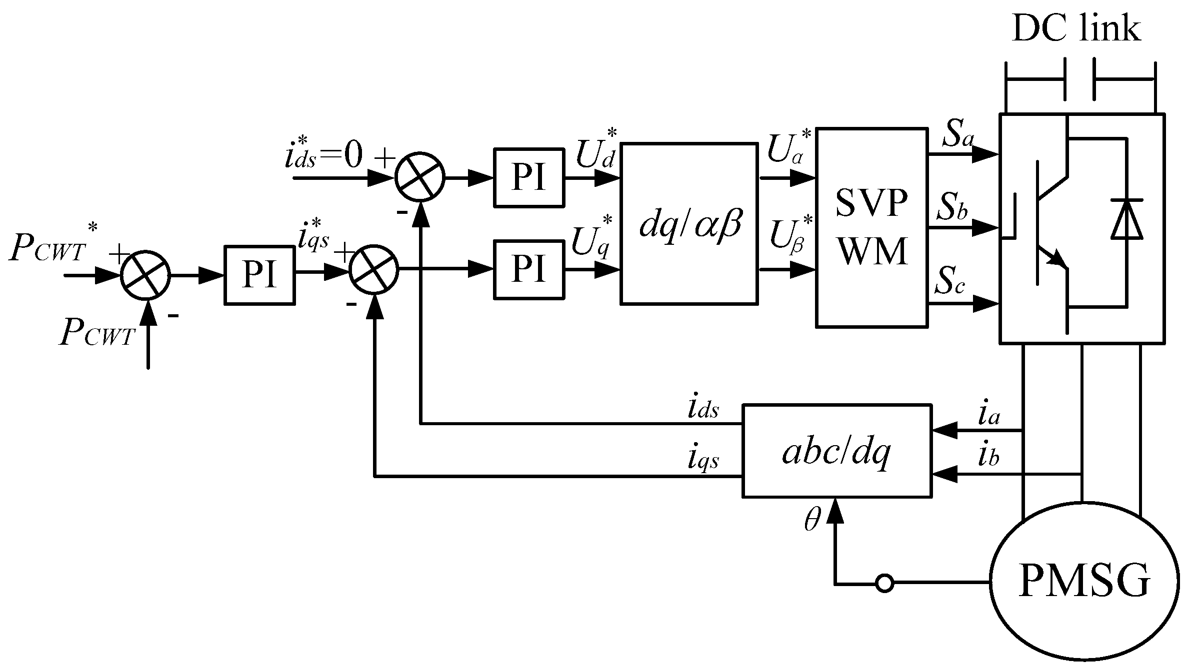
3.3. Control Strategy for the CWTs

The reference power given control method was adopted for the CWTs and its control diagram is shown in Figure 6. When the control target of the CWTs was the MPPT control, the reference power will be set to the maximum power according to Equation (5). When the target is changed to smooth output power, the reference power will be obtained according to the block diagram shown in Figure 4. The given power and the actual power were compared and the difference was adjusted by the PI module to obtain the q-axis current. The reference d-axis current was set to zero to simplify the control. Similar to the control of PWTs, the SVPWM method was applied in the CWTs control, as shown in Figure 7.

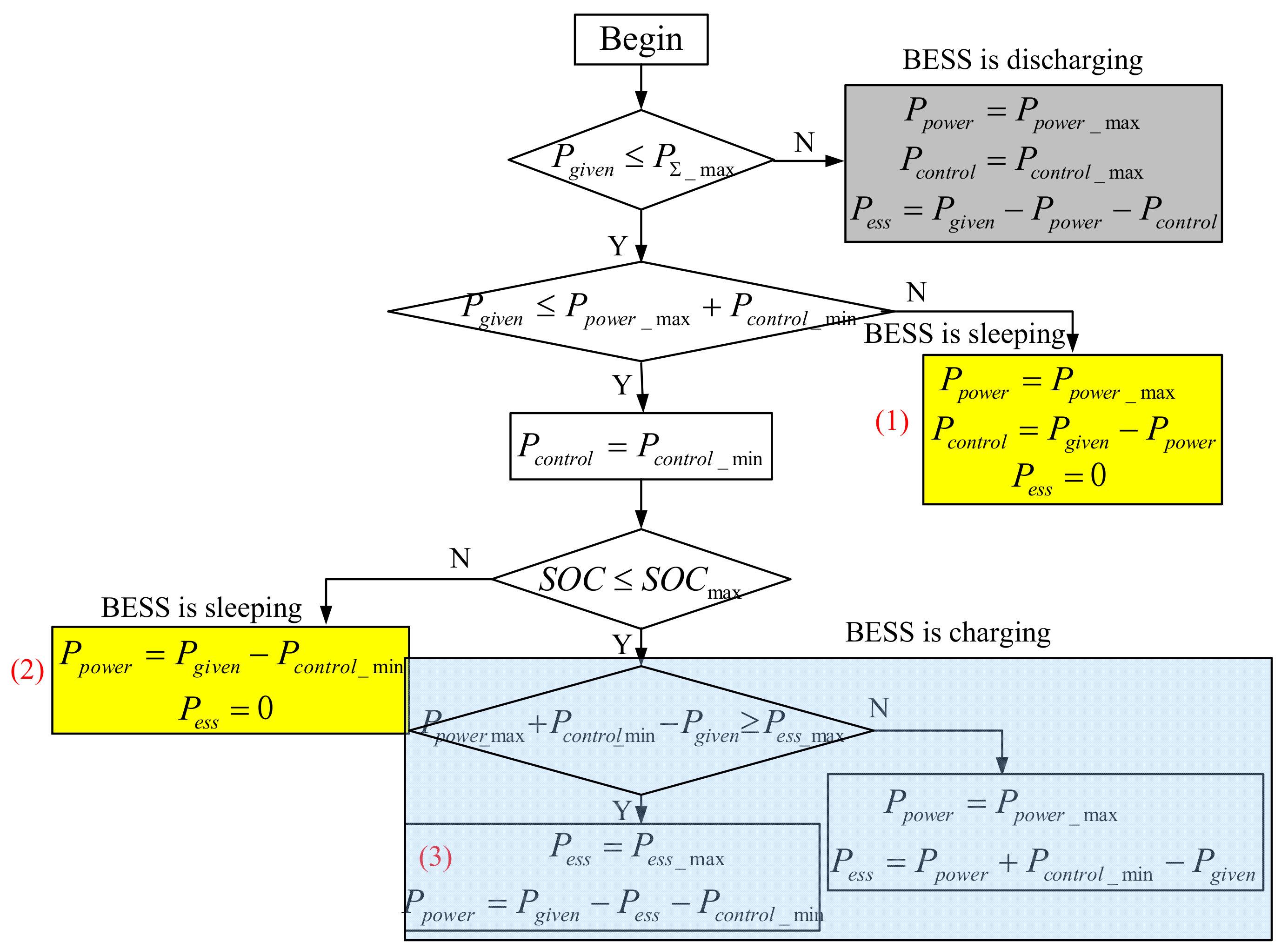
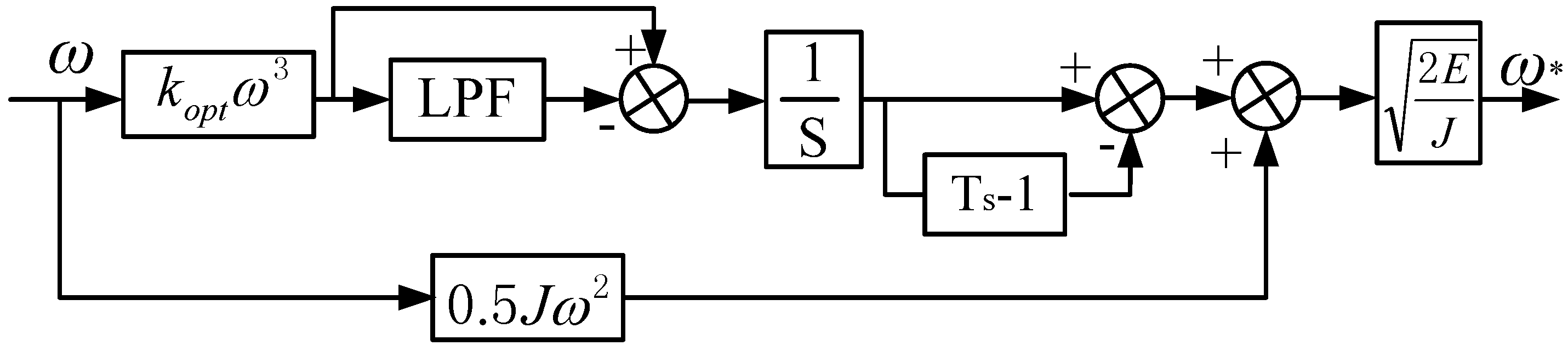
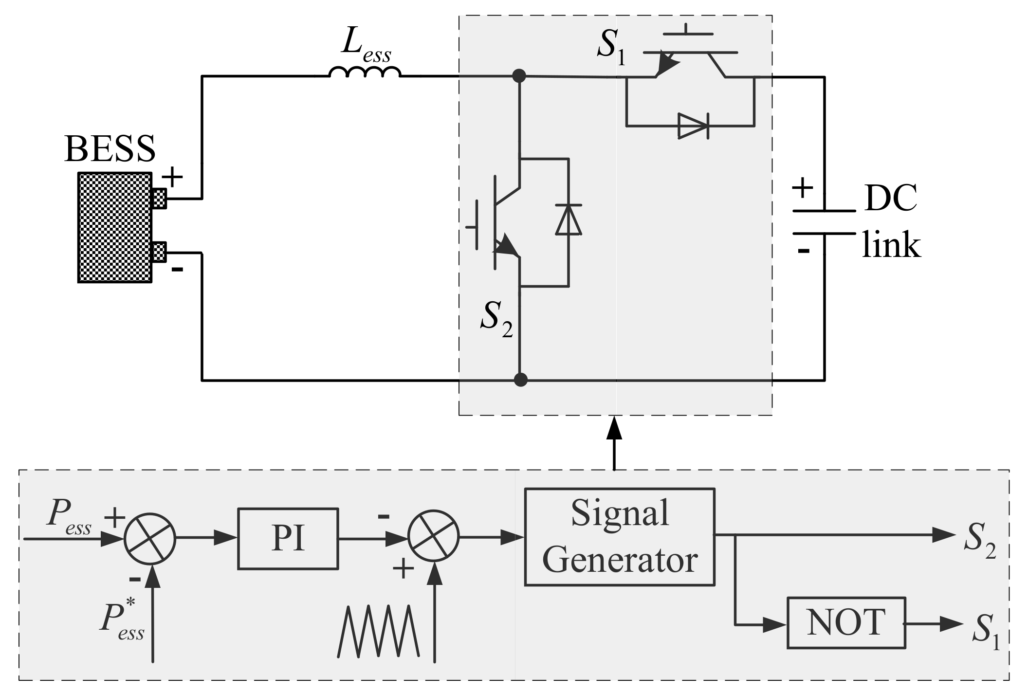
3.4. Control Strategy for the BESS

The BESS adopted in this paper was the backup support of CWTs to satisfy the high power requirements of the grid. As analyzed in Section 3.1, the charge and discharge times of the BESS were less than those of the BESS used in the traditional BESS based power smoothing control strategy. The BESS was connected to the HVDC DC link with a two-quadrant DC/DC converter, as shown in Figure 8. The DC/DC converter can work in both buck and boost modes according to the switch conditions of the two Insulated Gate Bipolar Transistors (IGBTs) S1 and S2. The duty ratios of switches S1 and S2 were controlled to regulate the power flow between output power of the nine WTs and grid demand power. The reference power of the BESS was obtained according to Figure 4.
When output power of the nine WTs was higher than the grid demand power, the redundant power will be absorbed in the BESS. Then S1 was controlled to be activated and the BESS was charged, while the DC/DC converter operated in the buck mode. On the contrary, when the output power of the nine WTs was lower than the grid demand power, S2 will be in the turn-on operation and the BESS was discharged while the DC/DC converter operated in the boost mode.

3.5. Evaluation of the Power Efficiency

The efficiency of the power smoothing control method can be evaluated through the power smoothing function P*level and maximum energy function P*max, which are expressed as [5]:
P l e v e l = 0 t | d P o ( t ) d t | d t ;
P max = 0 t P o ( t ) d t ,
where Po(t) is the output power at the time t.
If the power smoothing function P*level is small, the fluctuation of the output power is small. In other words, the performance of the power smoothing is great. The output power efficiency is also an important factor to power smoothing control method. The efficiency cannot be sacrificed too much for realizing the power smoothing. The larger the maximum energy function P*max is, the higher the output power efficiency is. Thus, the two factors will be calculated in the simulation to evaluate the effectiveness of proposed power smoothing control strategy.

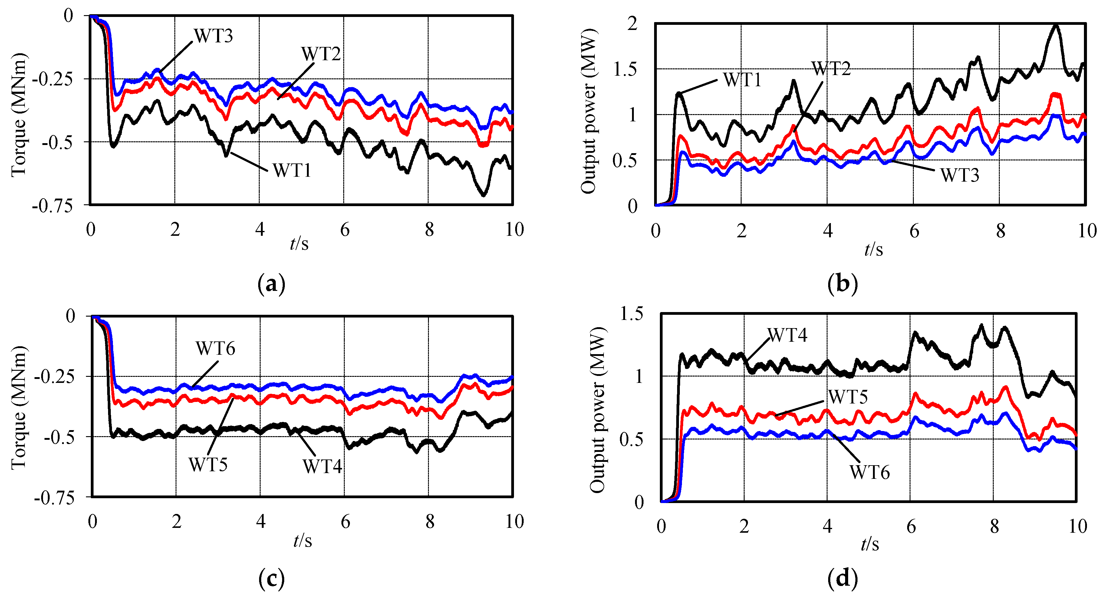
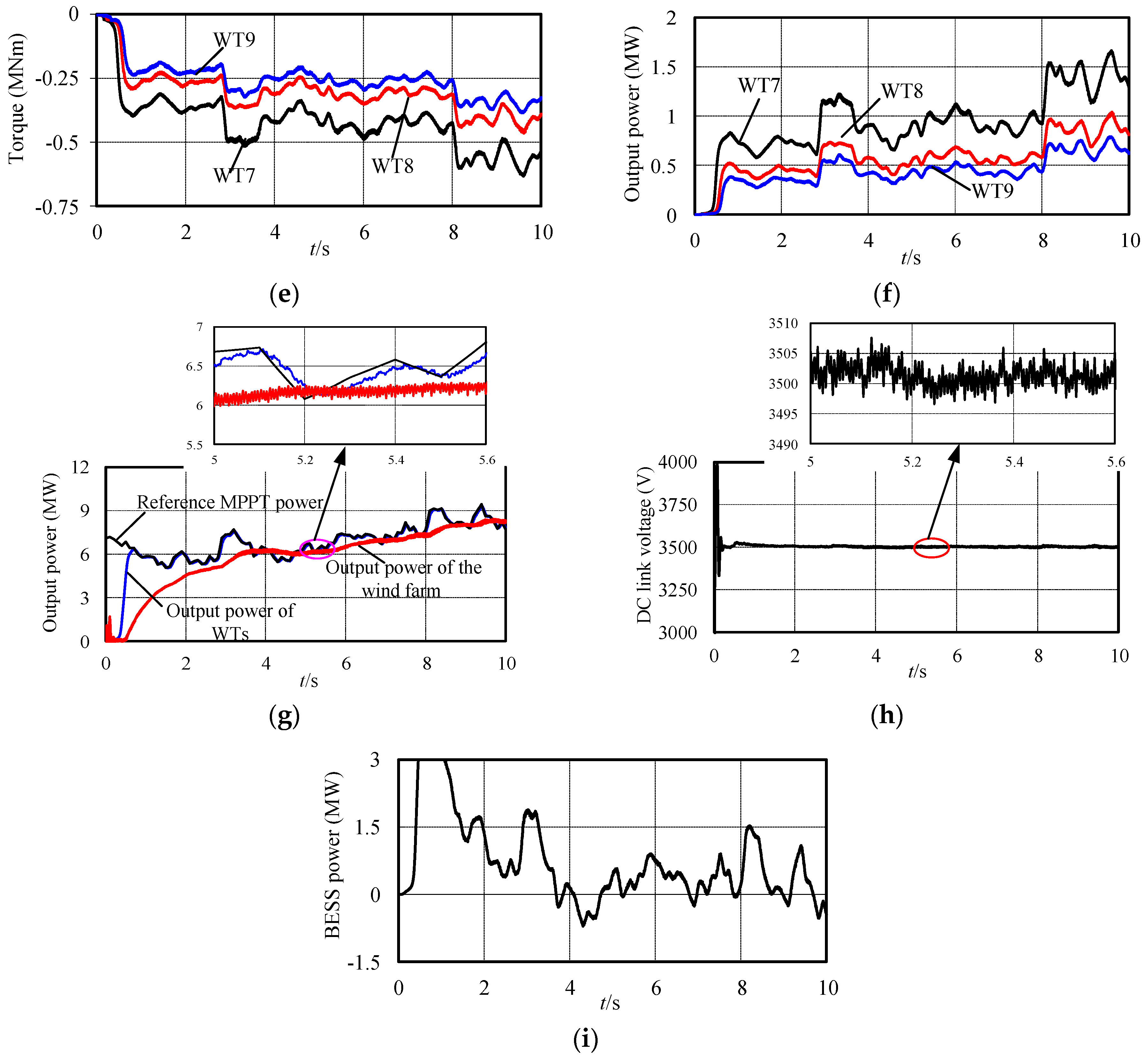
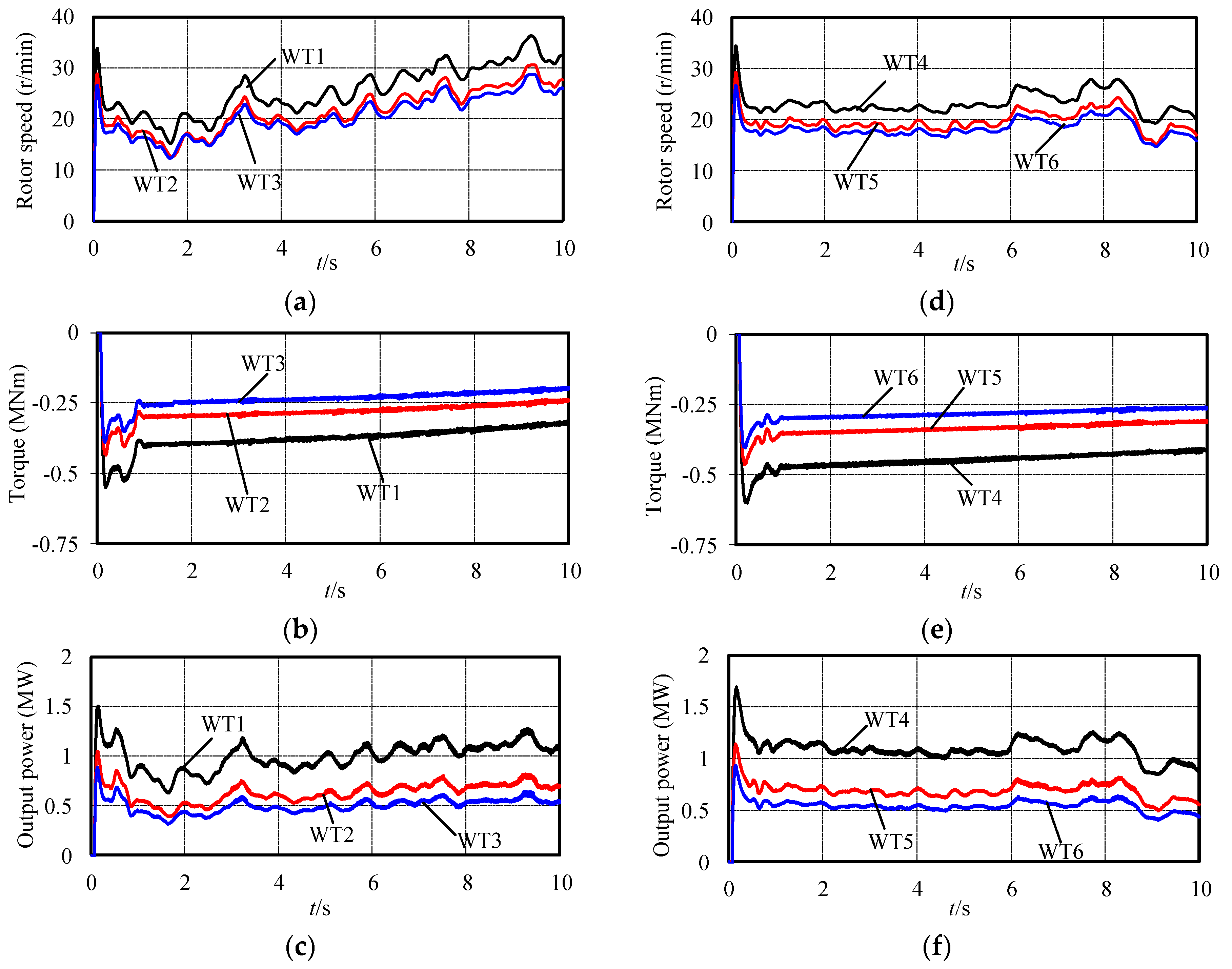
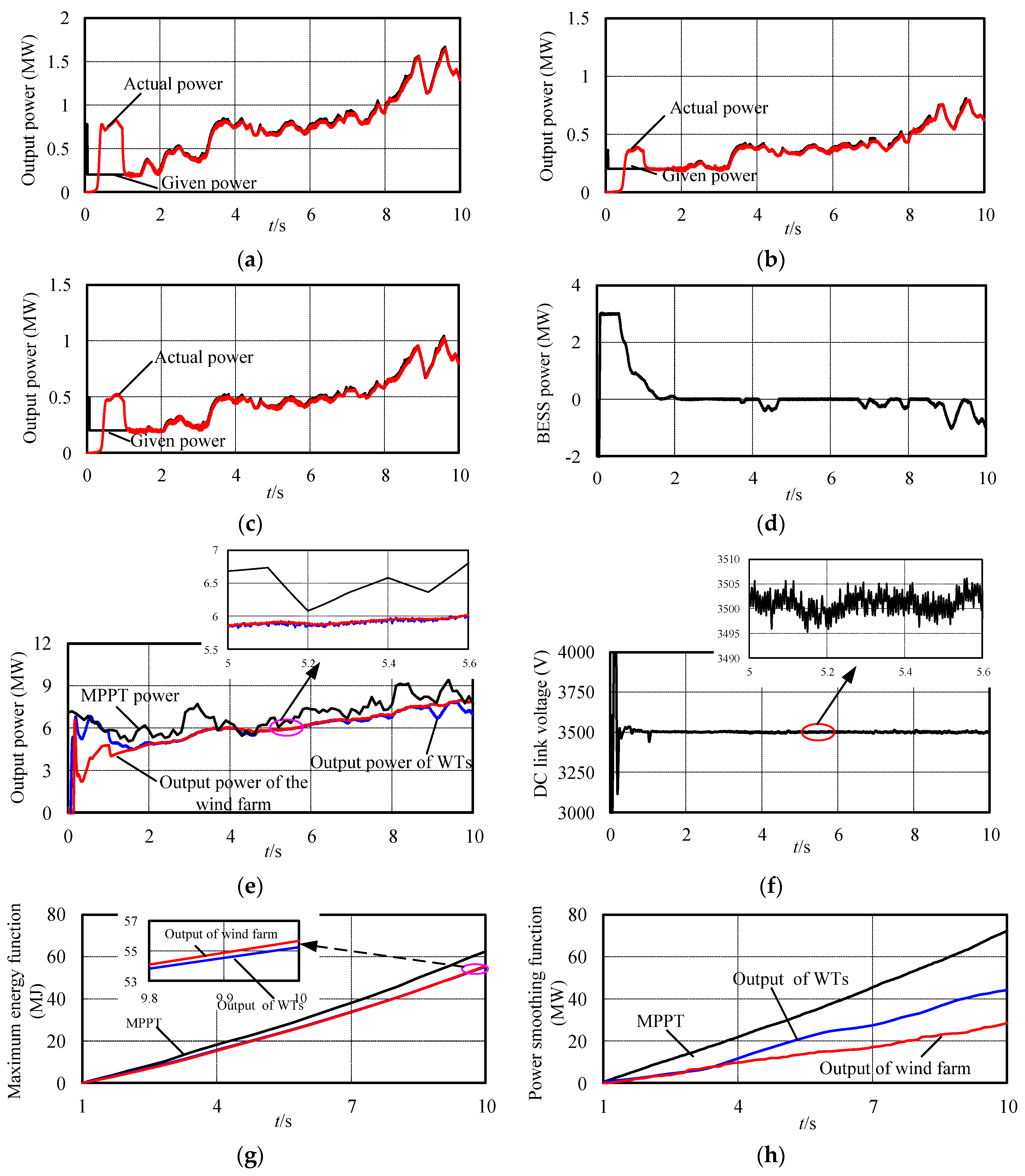
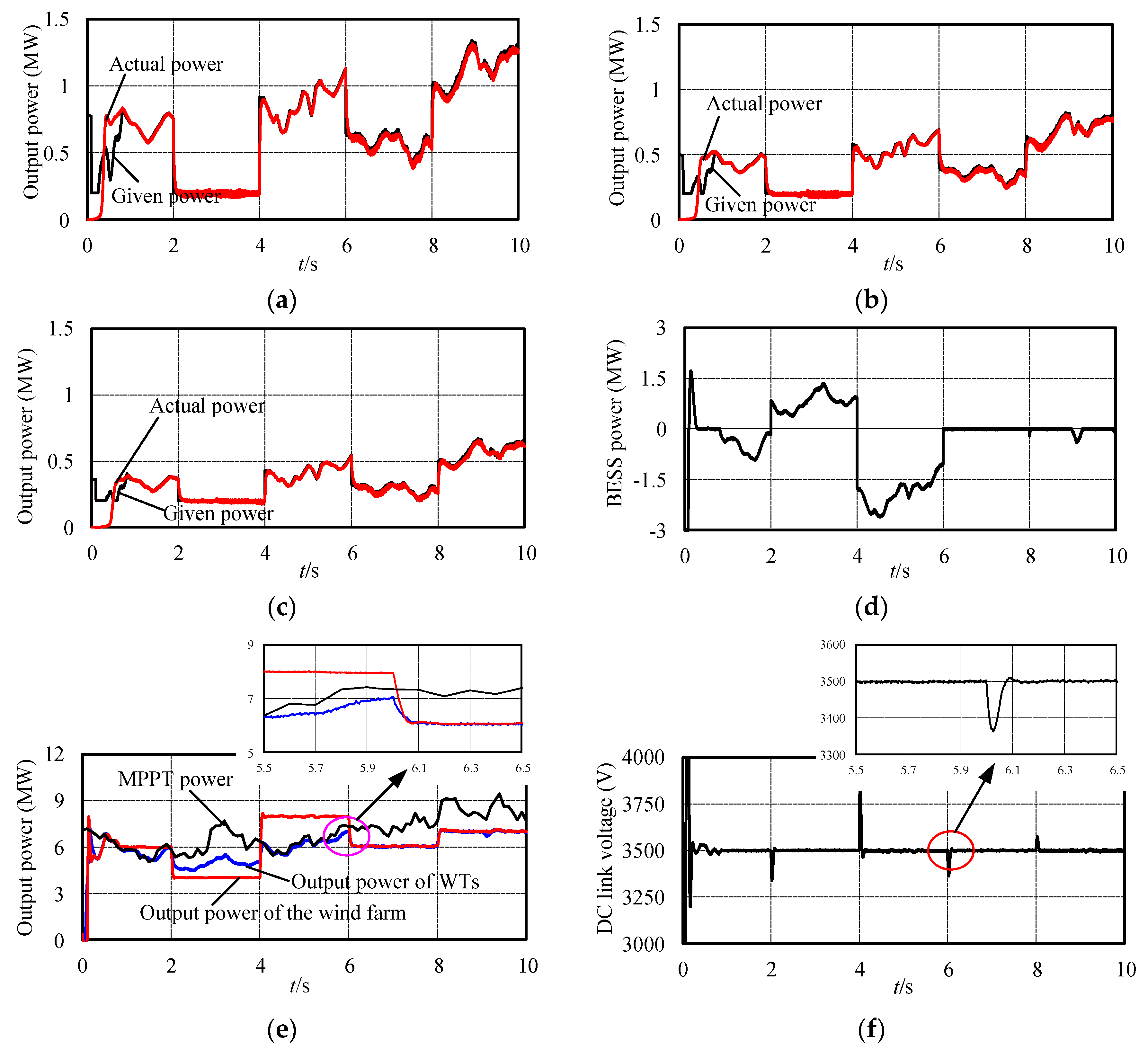
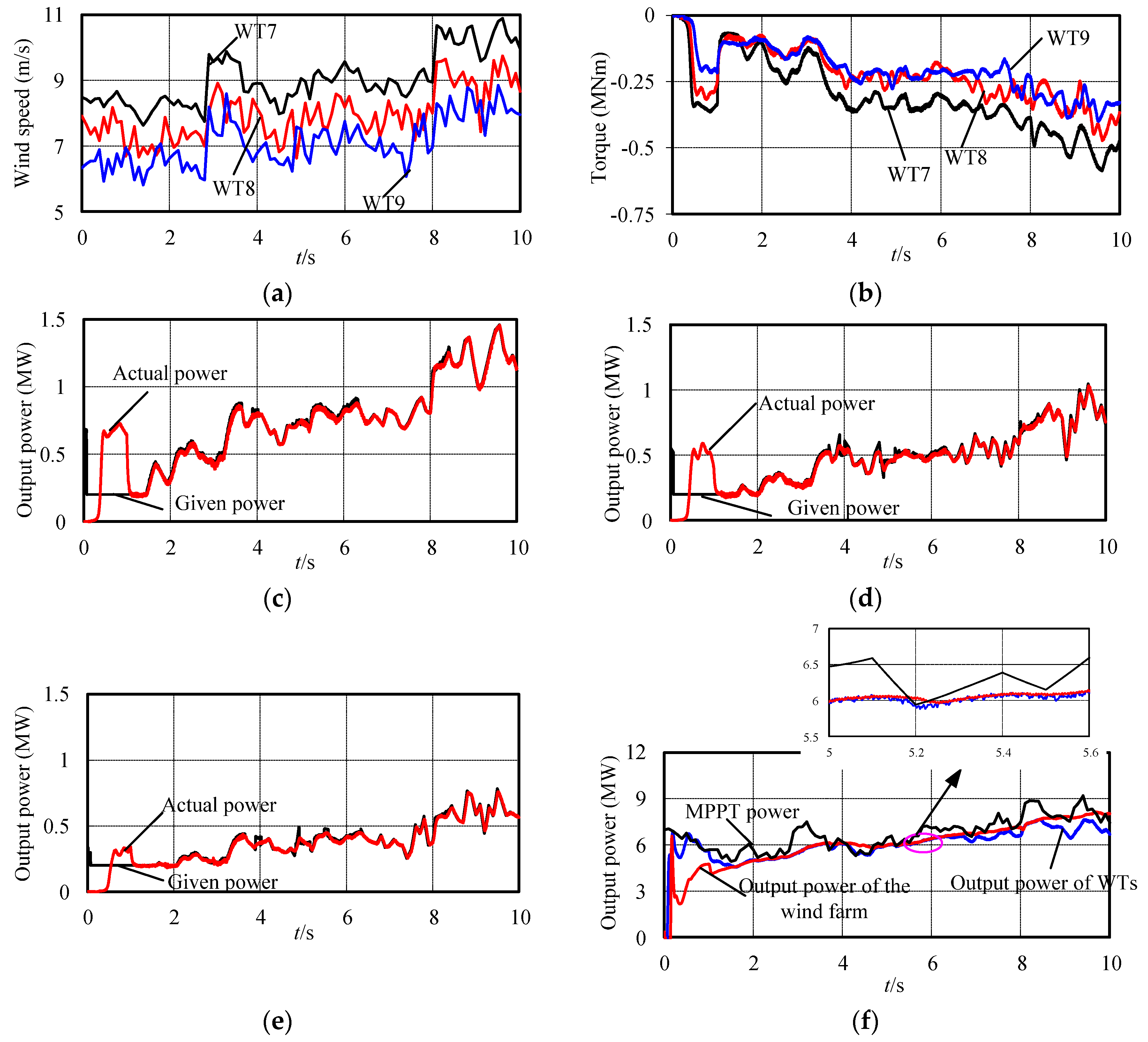
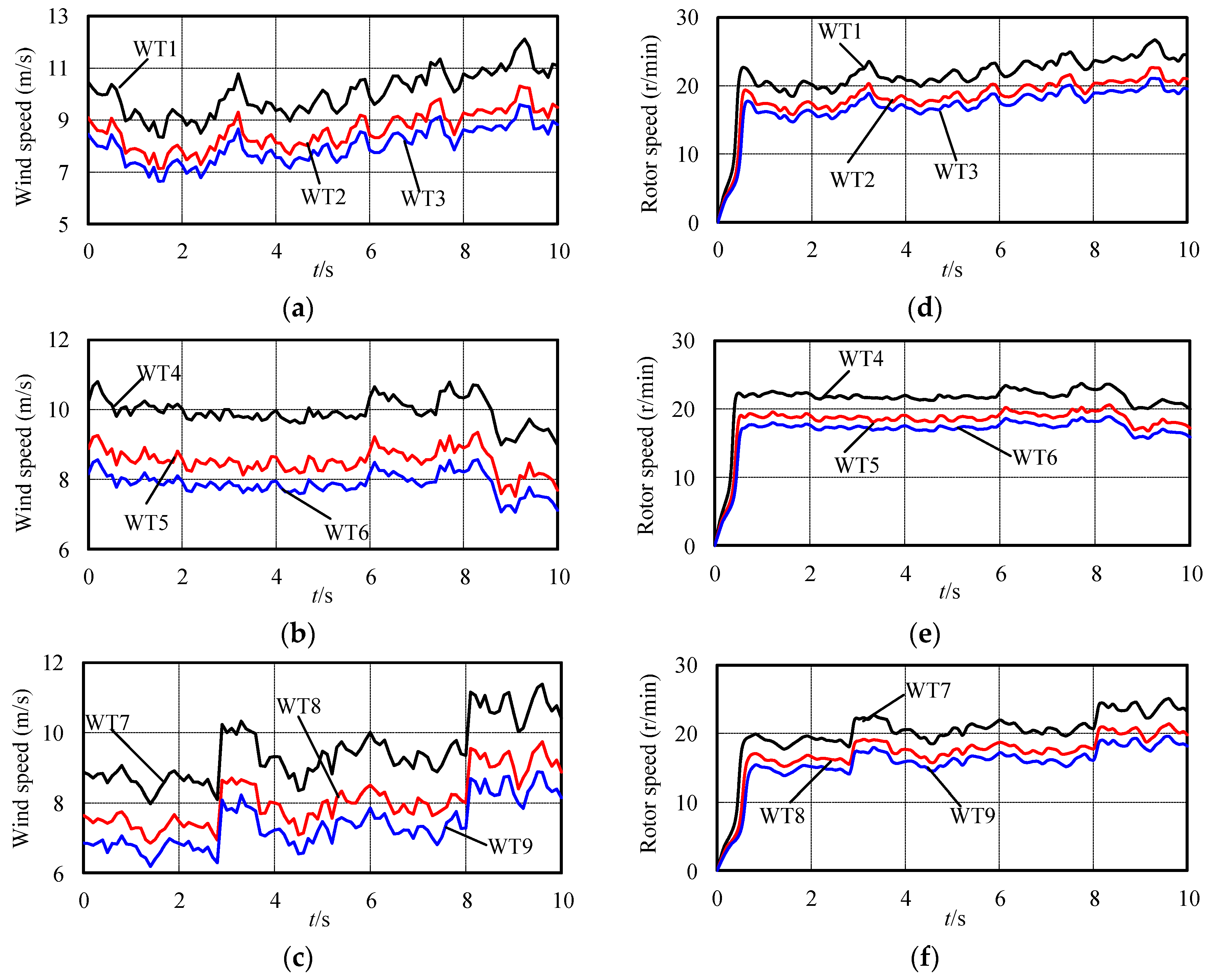
4. Simulation Results

The simulation model of the wind farm was built in the MATLAB/Simulink, which was based on the above-mentioned models and control strategies. The DC link voltage and the output reactive power were controlled through the grid-side converter. The variable pitch angle control was also applied in the simulation. The detailed control strategies of the grid-side converter and the pitch angle control were not presented in this paper and the detailed control strategy can be seen in [30,31]. The phase-locked-loop method was used to detect the grid voltage and phase information [32]. The parameters of the wind turbine and the PMSG are listed in Table 1. The size of the grid-side DC/AC inverter was chosen as 4.16 kV/20 MW which was based on the whole output power capacity of the wind farm (18 MW) by adding some margin. The reference voltage of the HVDC was set to 3500 V and the reference reactive power of the grid-connected inverter was set to zero. The minimum output power of CWTs was set as 200 kW. The size of the BESS was chosen according to the grid demand and the output power of wind turbines, which can be estimated from the wind speed. The small capacity BESS with the parameter 4 MW/3 MWh was configured in the simulation.
Three working modes of the wind farm were studied in the simulation, which were the MPPT mode, the power smoothing mode, and the specified power output mode, respectively. The first working mode of the wind farm was to output the maximum power then the optimum power given MPPT control was adopted for all the nine WTs, while using the control diagram shown in Figure 7. The BESS was adopted to smooth the output power of the nine WTs based on the traditional method. The reference power of the BESS was given as the difference of the output power of WTs and the output power through a low-pass filter. The simulation results of the WTs under the MPPT control are shown in Figure 9 and Figure 10.
The stochastic nature of the wind speed generated by the software TurbSim was given in the simulation. The wind speed waveforms of the nine turbines are shown in Figure 9a–c, while those of 1–3 WTs are given in Figure 9a, 4–6 WTs are given in Figure 9b and 7–9 WTs are given in Figure 9c. The wind speed of each wind turbine was given different values by considering the wake effect to close to the real wind farm in the simulation. The wind speeds of three group wind turbines were totally different, while the wind speed of each wind turbine in one group was decreasing from the upstream to downstream with the similar shape. Figure 9d–f show the rotor speed of the nine WTs respectively. It can be seen that the rotor speeds of nine WTs varied with the wind speeds to realize the MPPT control.
The torque of nine WTs is shown in Figure 10a,c,e and the output power is shown in Figure 10b,d,f, respectively. The MPPT control was realized while the torque and output power of the WTs varied with the wind speed. The total output power is shown in Figure 10g and it is clearly observed that the output power was consistent with the ideal MPPT power by ignoring the system losses in the simulation. The output power of the wind farm was smoothed by the BESS, as shown in Figure 10g. The power of the BESS was presented in Figure 10i, where the BESS was charging when the value was greater than 0 and discharging when the value was less than 0. It can be seen that the BESS was charging and discharging all the time under the traditional power smoothing control, which would cause the life of BESS to decrease seriously. Figure 10h demonstrates the DC link voltage of the wind farm, from which it can be seen that the voltage remained at the reference value 3500 V only, with little fluctuation which was about 5 V in the steady state, as shown in the extended waveform. Then the control strategy of the grid-side converter was verified.
The second working mode of the wind farm was to output the smoothing power and the simulation results are shown in Figure 11 and Figure 12. At this time, the proposed power smoothing control strategy based on the allocation and rotor inertia of wind turbines was adopted. The MPPT method combing the rotor inertia control was applied to the PWTs 1–6, while the given power control was adopted for the CWTs 7–9. The sampling period of the kinetic energy based power smoothing strategy for PWTs was 0.001. The cut off frequency of the low-pass filter was 10 Hz. The simulation waveforms of the PWTs are shown in Figure 11 including the rotor speed, torque, and output power. The rotor speed of PWTs shown in Figure 11a,d did not follow the optimum MPPT speed, which are shown in Figure 9d,e. It can be seen from Figure 11b,e that the torque of the PWTs was almost straight with very tiny fluctuations. Then, the mechanical stress of WTs was reduced effectively. By comparing the output power Figure 11c,f with Figure 10d,e, it can be observed that the output power of PWTs under the proposed rotor inertia based method was smoother than the power under MPPT control. Thus, the effectiveness of power smoothing method for PWTs based on the rotor inertia control was verified.
The output power of the three CWTs is shown in Figure 12a–c respectively. The reference power calculated according to the block diagram in Figure 4 was given to CWTs after 1s, while the maximum power was given to the PWTs before 1s. The power of each CWT was allocated according to the wind speed relationship which was obtained by calculating the wake effect. As shown in Figure 12a–c, the output power of CWTs was different from that under the MPPT control mode which is shown in Figure 10f and the actual output power of the three CWT can match the reference given power well. It can be seen from Figure 12e that the output power of WTs was smoothed through the proposed control strategy by comparing with the MPPT power. However, the output power of WTs could not be smoothed when the needed smoothing power exceeded the maximum output power of CWTs. In this case, the BESS was joined in to smooth the rest power and the power of BESS is shown in Figure 12d. Thus, the output power of the wind farm was smoother than the output power of WTs. Figure 12d shows that the BESS was not working all the time and then the charge and discharge times was reduced significantly compared to that using the traditional power smoothing method (shown in Figure 10i). Thus, the battery lift would be extended greatly. The DC link voltage can remain constant as shown in Figure 12f with little fluctuation around 5 V in the steady state.
The maximum energy function of the MPPT power, the output power of WTs and output power of the wind farm is shown in Figure 12g. It reflects that the maximum energy function of the output power of wind farm was slightly less than the MPPT output power. The energy loss mainly happened in the PWTs by adopting the kinetic energy based power smoothing control. The power smoothing function is shown in Figure 12h, from which it can be seen that the value of output power by WTs was obviously smaller than that of MPPT control. Then, it can be summarized that the proposed method can realize the good performance of power smoothing. The power smoothing effect was better when the BESS is joined in as shown in Figure 12h.
In some situations, the grid needs the wind farm to have the ability to output the specified power to meet the balance of the grid and loads. Thus, the third working mode of the wind farm was to output the determined power. The step-changed power demand (6 MW, 4 MW, 8 MW, 6 MW, 7 MW) for the wind farm was given in the simulation. The reference demand power was given to test the effectiveness of the proposed method in both cases of power increasing and power decreasing. Besides, the maximum reference demand power is limited by the sum of the maximum output power of wind turbines and the BESS. The simulation results of this case are shown in Figure 13. Being the same as that in the second working mode, the CWTs were given the reference power calculated according to block diagram Figure 4 after 1 s. The simulation results of PWTs were the same as that shown in Figure 11 and not given here. The output power of CWTs is demonstrated in Figure 13a–c, from which it can be seen that the CWTs outputted constant minimum power 200 kW between 2 s to 4 s due to the low grid demand power. The power of the BESS is shown in Figure 13, and it can be found that the BESS was working in the charge, discharge, and rest working modes according to the different power grid demands. The output power of the wind farm can follow the given step-changed demand power as shown in Figure 13e. As displayed in Figure 13f, the DC link voltage basically remained at the reference value, but with acceptable mutation due to the sudden power changes.
The new wind speed condition of CWTs was given in the simulation to increase persuasion of the proposed power smoothing strategy, while the wind speed of the PWTs was the same as that in Figure 9. The wind speed of CWTs is shown in Figure 14a, from which it can be seen that the shape of downstream WT was different from the upstream WT. Then, the rotor torque of each CWT had different shapes, as demonstrated in Figure 14b. The actual output power of the three CWT can match the reference given power well as shown in Figure 14c–e. Figure 14f shows the output power of the wind farm and it can be observed that the output power was smoothed by comparison with the reference MPPT power.
Thus, the proposed power smoothing control strategy through the reasonable allocation of the WTs in the wind farm and the rotor inertia was verified by the simulation results. The rotor inertia based power smoothing method for PWTs can reduce the torque ripple and mechanical stress significantly. The CWTs can output the appropriate power according to the reference value. The configured BESS were not working all the time to extend the life. The control for the grid-side converter was also verified through the constant DC link voltage. The proposed control strategy can respond to different needs of the grid, which was verified by the simulation results under different working modes.

5. Conclusions

This paper proposed a novel power smoothing control strategy for the wind farm by using the allocation of wind turbines. The WTs of the wind farm are divided into two classes: CWTs and PWTs with different control strategies. The PWTs were controlled to output the maximum power by combining with the rotor inertia based power smoothing method. Power given control was applied to the CWTs. The CWTs and small capacity BESS worked together to take charge of the total power output of the wind farm. The BESS was controlled to participate only when the power limit of CWTs was reached to reduce the charge and discharge times.
The wind farm model was built based on Matlab/Simulink to verify the proposed power smoothing control strategy by considering the wake effect. The grid-connected converter control was also adopted to fulfill the complete functionality of the wind farm. Three working modes of the wind farm as the MPPT control, power smoothing control, power given control are given in the simulation. It has been shown that the output power can meet the different needs of the grid. The effectiveness of the proposed power smoothing strategy was verified by the simulation results.

Author Contributions

Y.Z. was in charge of the work listed as: conceiving and proposing the control strategies, designing the simulations, making charts and writing the paper; H.Z. analyzed the simulation data and drew some of the charts. L.C. and S.G. analyzed and confirmed the simulation parameters, diagrams and results.

Acknowledgments

This work was supported in part by the National Natural Science foundation of China (51507050), the Natural Science foundation of Jiangsu Province (BK20150822), the Fundamental Research Funds for the Central Universities (Project No. 2018B15314) and Science and Technology Project of SGCC (J2017071).

Conflicts of Interest

The authors declare no conflicts of interest. The founding sponsors had no role in the design of the study; in the collection, analyses, or interpretation of data; in the writing of the manuscript, and in the decision to publish the results.

References

  1. Cheng, M.; Zhu, Y. The state of the art of wind energy conversion systems and technologies: A review. Energy Convers. Manag. 2014, 88, 332–347. [Google Scholar] [CrossRef]
  2. Muyeen, S.M.; Takahashi, R.; Murata, T.; Tamura, J. A variable speed wind turbine control strategy to meet wind farm grid code requirements. IEEE Trans. Power Syst. 2010, 25, 331–340. [Google Scholar] [CrossRef]
  3. Uehara, A.; Pratap, A.; Goya, T.; Senjyu, T.; Yona, A.; Urasaki, N.; Funabashi, T. A coordinated control method to smooth wind power fluctuations of a PMSG-based WECS. IEEE Trans. Energy Convers. 2011, 26, 550–558. [Google Scholar] [CrossRef]
  4. Aigner, T.; Jaehnert, S.; Doormain, G.L.; Gjengedal, T. The effect of large-scale wind power on system balancing in Northern Europe. IEEE Trans. Sustain. Energy 2012, 3, 751–759. [Google Scholar] [CrossRef]
  5. Howlader, A.M.; Senjyu, T.; Saber, A.Y. An integrated power smoothing control for a grid-interactive wind farm considering wake effects. IEEE Syst. J. 2015, 9, 954–965. [Google Scholar] [CrossRef]
  6. Howlader, A.M.; Urasaki, N.; Yona, A.; Senjyu, T.; Saber, A.Y. A review of output power smoothing methods for wind energy conversion systems. Renew. Sustain. Energy Rev. 2013, 26, 135–146. [Google Scholar] [CrossRef]
  7. Simon, D.R.; Johan, D.; Johan, M. Power smoothing in large wind farms using optimal control of rotating kinetic energy reserves. Wind Energy 2015, 18, 1777–1791. [Google Scholar]
  8. Johan, M.; Simon, D.R.; Johan, D. Smoothing turbulence-induced power fluctuations in large wind farms by optimal control of the rotating kinetic energy of the turbines. J. Phys. Conf. Ser. 2014, 524, 012187. [Google Scholar] [Green Version]
  9. Rawn, B.G.; Lehn, P.W.; Maggiore, M. Disturbance margin for quantifying limits on power smoothing by wind turbines. IEEE Trans. Control Syst. Technol. 2013, 21, 1795–1807. [Google Scholar] [CrossRef]
  10. Varzaneh, S.G.; Gharehpetian, G.B.; Abedi, M. Output power smoothing of variable speed wind farms using rotor-inertia. Electr. Power Syst. Res. 2014, 116, 208–217. [Google Scholar] [CrossRef]
  11. Rijcke, S.D.; Tielens, P.; Rawn, B.; Hertem, D.V.; Driesen, J. Trading energy yield for frequency regulation: Optimal control of kinetic energy in wind farms. IEEE Trans. Power Syst. 2015, 30, 2469–2478. [Google Scholar] [CrossRef]
  12. Zou, J.; Peng, C.; Shi, J.; Xin, X.; Zhang, Z. State-of-charge optimizing control approach of battery energy storage system for wind farm. IET Renew. Power Gener. 2015, 9, 647–652. [Google Scholar] [CrossRef]
  13. Zhang, F.; Xu, Z.; Meng, K. Optimal sizing of substation-scale energy storage station considering seasonal variations in wind energy. IET Gener. Transm. Distrib. 2016, 10, 3241–3250. [Google Scholar] [CrossRef]
  14. Jayasinghe, S.D.G.; Vilathgamuwa, D.M. Flying supercapacitors as power smoothing elements in wind generation. IEEE Trans. Ind. Electron. 2013, 60, 2909–2918. [Google Scholar] [CrossRef]
  15. Muyeen, S.M.; Hasanien, H.M.; Al-Durra, A. Transient stability enhancement of wind farms connected to a multi-machine power system by using an adaptive ANN-controlled SMES. Energy Convers. Manag. 2014, 78, 412–420. [Google Scholar] [CrossRef]
  16. Hasanien, H.M. A set-membership affine projection algorithm-based adaptive-controlled SMES units for wind farms output power smoothing. IEEE Trans. Sustain. Energy 2014, 5, 1226–1233. [Google Scholar] [CrossRef]
  17. Diaz-Gonzalez, F.; Bianchi, F.D.; Sunper, A.; Gomis-Bellmunt, O. Control of a flywheel energy storage system for power smoothing in wind power plants. IEEE Trans. Energy Convers. 2014, 29, 204–214. [Google Scholar] [CrossRef]
  18. Islam, F.; Al-Durra, A.; Muyeen, S.M. Smoothing of wind farm output by prediction and supervisory-control-unit-based FESS. IEEE Trans. Sustain. Energy 2013, 4, 925–933. [Google Scholar] [CrossRef]
  19. Jiang, Q.; Hong, H. Wavelet-based capacity configuration and coordinated control of hybrid energy storage system for smoothing out wind power fluctuations. IEEE Trans. Power Syst. 2013, 28, 1363–1372. [Google Scholar] [CrossRef]
  20. Pucci, M.; Cirrincione, M. Neural MPPT control of wind generators with induction machines without speed sensors. IEEE Trans. Ind. Electron. 2011, 58, 37–47. [Google Scholar] [CrossRef]
  21. Rosyadi, M.; Muyeen, S.M.; Takahashi, R.; Tamura, J. A Design Fuzzy Logic Controller for a Permanent Magnet Wind Generator to Enhance the Dynamic Stability of Wind Farms. Appl. Sci. 2012, 2, 780–800. [Google Scholar] [CrossRef] [Green Version]
  22. Muyeen, S.M.; Hasanien, H.M. Operation and control of HVDC stations using continuous mixed p-norm-based adaptive fuzzy technique. IET Gener. Transm. Distrib. 2017, 11, 2275–2282. [Google Scholar] [CrossRef]
  23. Kim, H.; Singh, C.; Sprintson, A. Simulation and estimation of reliability in a wind farm considering the wake effect. IEEE Trans. Sustain. Energy. 2012, 3, 274–282. [Google Scholar] [CrossRef]
  24. Gil, M.P.; Gomis-Bellmunt, O.; Sumper, A.; Bergas-Jane, J. Power generation efficiency analysis of offshore wind farms connected to a SLPC (single large power converter) operated with variable frequencies considering wake effects. Energy 2012, 37, 455–468. [Google Scholar]
  25. Tian, J.; Zhou, D.; Su, C.; Soltani, M.; Chen, Z.; Blaabjerg, F. Wind turbine power curve design for optimal power generation in wind farms considering wake effect. Energies 2017, 10, 395. [Google Scholar] [CrossRef]
  26. Tian, J.; Zhou, D.; Su, C.; Blaabjerg, F.; Chen, Z. Optimal Control to Increase Energy Production of Wind Farm Considering Wake Effect and Lifetime Estimation. Appl. Sci. 2017, 7, 65. [Google Scholar] [CrossRef]
  27. Lee, J.; Muljadi, E.; Sorensen, P.; Kang, Y.C. Releasable kinetic energy-based inertial control of a DFIG wind power plant. IEEE Trans. Sustain. Energy 2016, 7, 279–288. [Google Scholar] [CrossRef]
  28. Hang, J.; Zhang, J.; Cheng, M.; Ding, S. Detection and discrimination of open phase fault in permanent magnet synchronous motor drive system. IEEE Trans. Power Electron. 2016, 31, 4697–4709. [Google Scholar] [CrossRef]
  29. Gupta, A.K.; Khambadkone, A.M. A general space vector PWM algorithm for multilevel inverters, including operation in overmodulation range. IEEE Trans. Power Electron. 2007, 22, 517–526. [Google Scholar] [CrossRef]
  30. Geng, H.; Yang, G. Output power control for variable-speed variable-pitch wind generation systems. IEEE Trans. Energy Convers. 2010, 25, 494–503. [Google Scholar] [CrossRef]
  31. Zhu, Y.; Zang, H.; Fu, Q. Grid-connected Control Strategies for a Dual Power Flow Wind Energy Conversion System. Electr. Power Compon. Syst. 2017, 45, 1–14. [Google Scholar] [CrossRef]
  32. Wang, Q.; Cheng, M.; Jiang, Y.; Zuo, W.; Buja, G. A simple active and reactive power control for applications of single-phase electric springs. IEEE Trans. Ind. Electron. 2018, 65, 6291–6300. [Google Scholar] [CrossRef]
Figure 1. Curve of Cp (λ, β).
Applsci 08 00980 g001
Figure 2. The layout of the wind farm model.
Applsci 08 00980 g002
Figure 3. The wake effect model. (a) Jensen model principle; (b) wind turbine distribution structure.
Applsci 08 00980 g003
Figure 4. Block diagram of the power allocation.
Applsci 08 00980 g004
Figure 5. Rotor inertial power smoothing control by adopting the low-pass filter.
Applsci 08 00980 g005
Figure 6. Control diagram of the power wind turbines.
Applsci 08 00980 g006
Figure 7. Control diagram of the control wind turbines.
Applsci 08 00980 g007
Figure 8. Structure and control of the energy storage system based on DC/DC converter.
Applsci 08 00980 g008
Figure 9. Time histories of the wind speed and rotor speed in the wind farm under the maximum power point tracking (MPPT) control. (a) Wind speed of the first group WTs (1–3). (b) Wind speed of the second group WTs (4–6). (c) Wind speed of the third group WTs (7–9). (d) Rotor speed of the first group WTs (1–3). (e) Rotor speed of the second group WTs (4–6). (f) Rotor speed of the third group WTs (7–9).
Applsci 08 00980 g009
Figure 10. Time histories of the torque, power of WTs in the wind farm under the maximum power point tracking (MPPT) operation mode. (a) Torque of the first group WTs (1–3). (b) Torque of the second group WTs (4–6). (c) Torque of the third group WTs (7–9). (d) Output power of the first group WTs (1–3). (e) Output power of the second group WTs (4–6). (f) Output power of the third group WTs (7–9). (g) Total output power. (h) DC link voltage. (i) Power of the BESS.
Applsci 08 00980 g010aApplsci 08 00980 g010b
Figure 11. Time histories of the PWTs in the wind farm under the power smoothing operation mode. (a) Rotor speed of PWTs (1–3). (b) Torque of PWTs (1–3). (c) Output power of PWTs (1–3). (d) Rotor speed of PWTs (4–6). (e) Torque of PWTs (4–6). (f) Output power of PWTs (4–6).
Applsci 08 00980 g011
Figure 12. Time histories of the CWTs and the wind farm under the power smoothing operation mode. (a) Output power of CWT (WT7). (b) Output power of CWT (WT8). (c) Output power of CWT (WT9). (d) Power of the BESS. (e) Total output power of the wind farm. (f) DC link voltage. (g) Maximum energy function. (h) Power smoothing function.
Applsci 08 00980 g012
Figure 13. Time histories of the wind farm under the specified power given operation mode. (a) Output power of CWT (WT7). (b) Output power of CWT (WT8). (c) Output power of CWT (WT9). (d) Total output power of the wind farm. (e) Power of the BESS; (f) DC link voltage.
Applsci 08 00980 g013
Figure 14. Time histories of the wind farm when the wind speed condition of CWTs is changed. (a) wind speed of CWTs. (b) Rotor torque of CWTs. (c) Output power of CWT (WT7). (d) Output power of CWT (WT8). (e) Output power of CWT (WT9). (f) Total output power of the wind farm.
Applsci 08 00980 g014
Table 1. Parameters of the simulation.
Wind Turbine PMSG
Blade radius (m)35Stator resistant (Ω)0.01
Air density (kg/m3)1.225Inductance (mH)0.835
Optimum TSR8.1Rotor inertia (kg·m2)8500
Optimum power coefficient0.48PM linkage (Wb)8.76
Rated wind speed (m/s)12Pole pairs32
Rated power (MW)2Rated power (MW)2

