Article

A New Closed-Form Solution for Acoustic Emission Source Location in the Presence of Outliers

1
School of Resources and Safety Engineering, Central South University, Changsha 410083, China
2
State Key Laboratory of Mining Disaster Prevention and Control Co-founded by Shandong Province and the Ministry of Science and Technology, Shandong University of Science and Technology, Qingdao 266590, China
*
Authors to whom correspondence should be addressed.
Appl. Sci. 2018, 8(6), 949; https://doi.org/10.3390/app8060949
Submission received: 21 April 2018 / Revised: 4 June 2018 / Accepted: 5 June 2018 / Published: 8 June 2018

Abstract

:
The accuracy of an acoustic emission (AE) source location is always corrupted by outliers due to the complexity of engineering practice. To this end, a preconditioned closed-form solution based on weight estimation (PCFWE) is proposed in this study. Firstly, nonlinear equations are linearized, and initial source coordinates are obtained by using equal weights. Residuals, which are calculated by source coordinates, are divided into three regions according to normal distribution. Secondly, the weight estimation is developed by establishing the relationship between residuals and weights. Outliers are filtered by the iteration between the weight estimation and source location. Subsequently, linear equations are reconstructed with the remaining measurements containing no outliers, while they are ill-conditioned. Finally, the preconditioning method is applied to weaken the ill condition of the reconstructed linear equations, so as to improve the location accuracy. This new method is verified by a pencil-lead break experiment. Tests results show that the location accuracy and stability of the new method are superior to traditional methods. In addition, outlier tolerance and the velocity sensibility of the new method are investigated by simulating tests.

1. Introduction

The acoustic emission (AE) source location method based on sensor array has been a hot research topic with widespread applications in many fields of structural health, underground tunneling, and deep mining [1,2,3,4,5,6,7]. Nevertheless, locating the source is not a simple task, because there are two major challenges, namely: measurement errors and real-time implementation [8,9,10,11,12].
The least squares principle, which is employed in most methods, can achieve a favorable location accuracy on the condition that all of the measurements are accurate or only have minor errors [13,14,15,16,17,18]. However, adding an outlier will cause the residual value to dramatically increase, which is enlarged due to the square nature of the least squares principle, and the location performance to significantly deteriorate [19,20]. Accurate estimation for the arrival times of acquired signals associated with each sensor is the underlying challenge for the most picking-based location method. Researchers have proposed varying algorithms, trying to pick arrivals accurately and in real-time, such as a short and long-time average ratio [21], higher order statistics method [22]. However, these methods only have good performances in clean or high signal-to-noise ratio environments. Niccolini et al. [23,24] proposed the joint autoregressive modeling of noise and the signal in windows using Akaike information criterion with an automatic procedure for signal data processing under a low signal-to-noise ratio environment. This method, which can eliminate certain false or doubtful arrivals before the source location, can be utilized to obtain the real-time arrivals and reduce the probability of an outlier. However, it does not mean that all of outliers will be eliminated, because there are other factors that can generate outliers besides the background noise. Practical applications of monitoring systems have reported that the sensors are easy to be triggered incorrectly by interference signals due to the complex engineering environment, which brings external outlier signals [25,26]. In addition, outliers can also occur in these cases, such as signal interference, sensor location errors, weak and ambiguous of arrivals, interchannel crosstalk, or simply hardware failure. Therefore, all the above cases may bring outliers in measurements, especially in the use of automated picking methods. Considering the difficult acquisition of an accurate measurement and the deterioration effect of the outliers on the source location, the error-tolerant location methods have been developed by scholars to reduce the influence of outliers [27,28].
A large amount of error-tolerant methods of time difference of arrival (TDOA) have been proposed, which can be classified into nonlinear methods and linear methods [29,30,31,32,33]. Nonlinear location methods, including maximum likelihood [34,35], the virtual field optimization method [36], and the least absolute deviation method [37], have been suggested to improve the error-tolerance. To gain the optimum solution of these nonlinear methods, iterative techniques should be used because of nonlinear TDOA equations. Alternative choices include the simplex method [38], Newton iterative method [39], and the Gauss–Newton method [40]. However, these methods not only require an appropriate guess of initial location near the true solution, which is difficult to obtain in practice, but also probably suffer from convergence problems and a large computational burden caused by the iterative nature. Compared with nonlinear methods, linear methods in the close form guarantee the convergence and real-time implementation. The weighted least squares algorithm, which gives different weights to different equations, is a generic form of the error-tolerant closed-form solution. Two-step weighted least squares (TSWLS), which linearizes the nonlinear TDOA equations by introducing an additional variable [41,42,43,44], is one of the prevalent weighted least squares methods. This method has been widely used in various fields as a benchmark for subsequent studies [9,31,45]. Firstly, source location and the additional variable are considered independent variables to conduct the estimation. Secondly, the estimation is developed by considering the relationship between the additional variable and the source location. However, the covariance matrix of measurement errors used in this location process is difficult to accurately estimate, which causes performance degradation at the source location [9]. Unlike the method of weight least squares, Dong et al. [46] recently proposed comprehensive closed-form solutions using a set of sensor networks and the logistic probability density function, so as to improve the location accuracy. However, location errors of the closed-form solution are still large, because only six sensors are considered in each calculation process, and the coefficient matrix of the linear equations is close to ill-conditioned. In addition, since many subsets of six sensors exist, it requires enormous computing power; thus, it has a poor performance in real-time implementation [47].
Aiming at improving the error-tolerance and real-time implementation of the AE source location, this paper proposes the preconditioned closed-form solution based on weight estimation (PCFWE) to seek the optimal source coordinates by filtering outliers and reducing the ill condition of linear equations. PCFWE is also compared with the TSWLS [41] and linear least squares (LLS) methods. The effectiveness and accuracy of the proposed PCFWE are verified by the pencil-lead break experiment and simulating tests. In Section 2, the ordinary closed-form method that fairly treats all of the measurements is stated. In Section 3, the theory of the proposed method is formulated mathematically. In Section 4, the location results of the pencil-lead break experiment are reported. Finally, outlier tolerance and the velocity sensibility of the proposed method are discussed and concluded in Section 5.

2. Ordinary Closed-Form Method

To achieve an accurate and real-time AE source location, many closed-form methods exploiting the LLS principle are proposed [15,16,48,49]. The process of the ordinary closed-form location method mainly contains two steps as follows. Firstly, nonlinear equations are transformed into linear forms to reduce the difficulty in solving nonlinear equations by iterative methods. Secondly, the LLS principle is incorporated to solve the overdetermined liner equations, which can use as many measurements as possible, and yield a better location accuracy than those that only use a minimum number of measurements [50,51], i.e., the number of equations is equal to the number of unknowns. From the viewpoint of error control, the dataset is statistically more reliable, and the array geometry is more reasonable when more measurements are used. The process of an ordinary closed-form location method with the LLS principle is stated as follows.
Assuming that an AE source is located at source θ (x, y, z), and the n + 1 sensors are located at Si (xi, yi, zi) (i = 0, 1, ···, n), for an arbitrary AE event, the source coordinates satisfy the following control equations:
( x i x ) 2 + ( y i y ) 2 + ( z i z ) 2 = v 2 ( Δ t i + t 0 ) 2
where t0 is the propagation time of the acoustic wave from the source to the nearest sensor. The sensors are numbered Si (i = 0, 1, ···, n) according to the arrival orders of the AE signal. The nearest sensor S0 that receives the AE signal first is regarded as the reference sensor. Δ t i is the time difference between reference sensor S0 and sensor Si (i = 1, 2, ···, n), namely the time difference of arrival (TDOA). Besides, when i = 0 , Δ t i = 0 , nonlinear equations can be linearized by subtracting the equation i = 0 from i ≥ 1.
2 ( x i x 0 ) x + 2 ( y i y 0 ) y + 2 ( z i z 0 ) z + 2 Δ t i v 2 t 0 = L i , i = 1 , 2 , n
where L i = x i 2 x 0 2 + y i 2 y 0 2 + z i 2 z 0 2 Δ t i 2 v 2 .
Equation (2) can be expressed in matrix form as:
A θ = b
where A = 2 [ x 1 x 0 y 1 y 0 z 1 z 0 Δ t 1 v 2 x 2 x 0 y 2 y 0 z 2 z 0 Δ t 2 v 2 x n x 0 y n y 0 z n z 0 Δ t n v 2 ] , θ = [ x y z t 0 ] , b = [ L 1 L 2 L n ] .
To find the location parameters θ in Equation (3), which minimizes the sum of the residual square for the linear equation system:
arg min θ | | b A θ | | = arg min θ i = 1 n ( b i A i θ ) 2
The closed-from solution with the least squares principle can be obtained by:
θ = ( A T A ) 1 A T b
where the symbol T denotes the matrix transpose, and ATA is the Hessian matrix.
The solution of LLS is the best linear unbiased estimator for the AE source location when the measurement errors are independent and identically distributed. However, it may produce dramatic location errors due to the equal treatments of all of the measurements, even the outliers. Therefore, outliers are considered to be filtered by weight estimation first; then, linear equations are reconstructed with the remaining measurements that contain no outliers to obtain more accurate location results. However, the linear equation system (3) is always close to ill-conditioned, which can cause a large location error with a minor disturbance. Therefore, the preconditioning of linear equations is adopted to weaken the ill condition and further improve the location accuracy.

3. Theory of Proposed Method

To solve the above problems, the PCFWE method is proposed to seek the optimal location results. The proposed method mainly includes two processes: filtering the outliers by weight estimation and reconstructing the linear equations with remaining measurements.

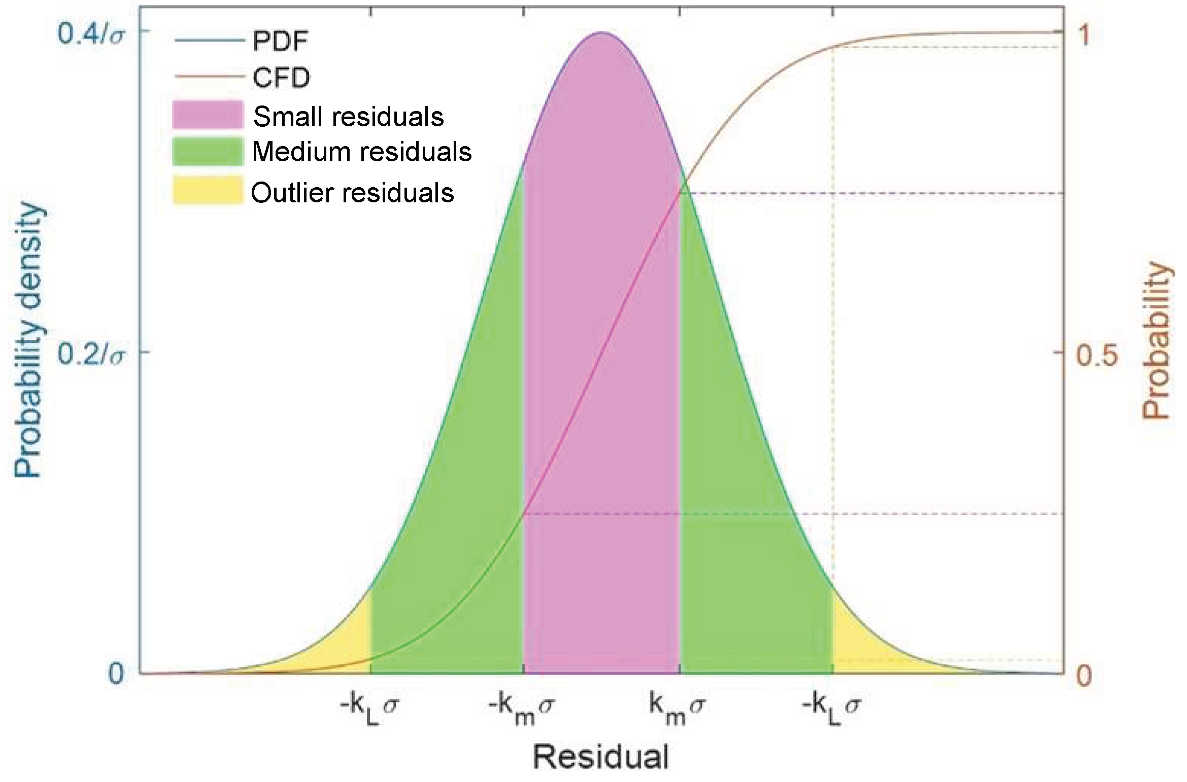
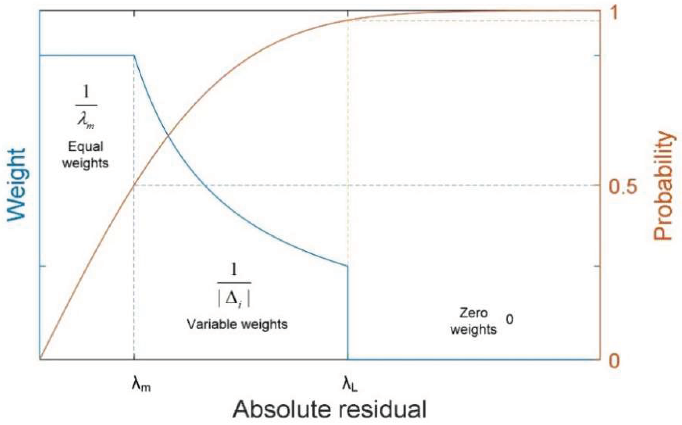
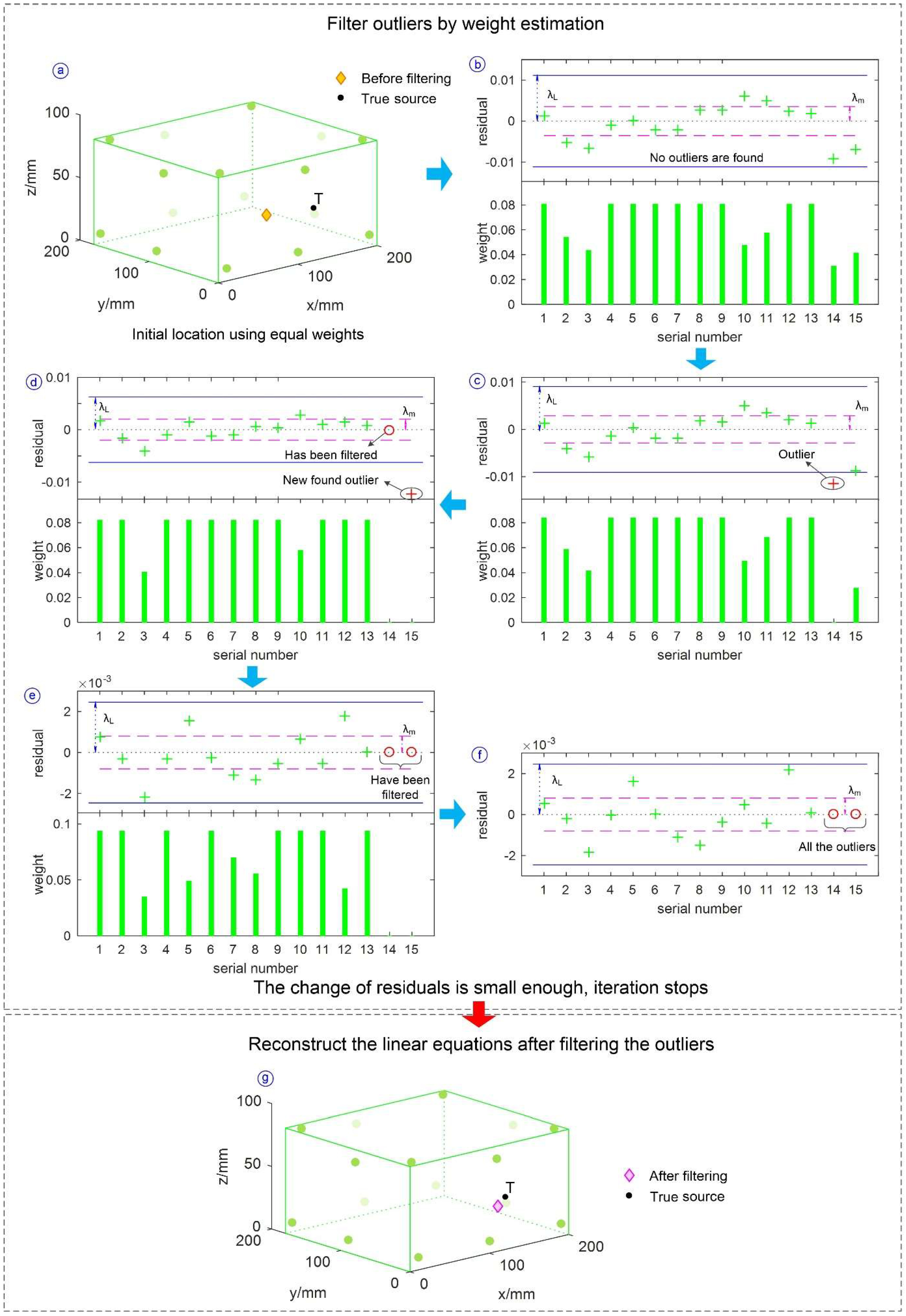
3.1. Filtering Outliers by Weight Estimation

3.1.1. Weight Estimation

The main idea of weight estimation is that a small weight is given to the measurement with a large residual, which in turn will reduce the influence of the outlier. Therefore, it is crucial to establish the relationship between weights and residuals.
However, the residuals of the real model cannot be obtained directly, so the weights are also difficult to be determined. In this work, the AE source is located by the LLS method, and each measurement is treated with equal weights firstly. Then, the residuals of the fitting model can be obtained and used to replace the residuals of the true model:
Δ i = b i A i θ , i = 1 , 2 , , n
where, Δ i is the ith element of a residual vector of the fitting model.
After obtaining the residuals, the weight estimation is developed by establishing the relationship between weights and residuals. The simplest method is to exploit the reciprocal value of the residuals as the weights directly. However, when a residual tends to be zero, the corresponding measurement is assigned with an unreasonably high weight, resulting in overfitting. Therefore, the weight should have a maximum upper limit to avoid overfitting, which can be realized by setting a lower limit of λm. Second, residuals exceeding the threshold λL are considered outliers, and the relative measurements are also regarded as outliers and filtered by setting the weight to zero. Therefore, the weight estimation can be expressed as follows [52]:
w i = { 1 / λ m , i f | Δ i | λ m 1 / Δ i , i f λ m < | Δ i | < λ L 0 ,    e l s e
To determine the specific parameters of the weight estimation, it is assumed that residuals obey the normal distribution. Therefore, the threshold λ m and λ L in (7) can be defined by:
λ m = k m σ
λ L = k L σ
where k m and k L are the correlation factors, and σ is the estimated value of the standard deviation of residuals, with expression as follows:
σ = 1 n m i = 1 n w i ( b i A i θ ) 2 1 n i = 1 n w i
where m is the number of the unknown parameters. The denominator 1 n i = 1 n w i is used to standardize the weights.
Figure 1 shows the regional division of residuals according to the normal distribution. The parameters k m and k L divide the complete residuals into three regions, including minor residuals, medium residuals, and outlier residuals. Besides, the corresponding weights transformed from these residuals are divided into three parts, including an equal weight part, a variable weight part, and a zero weight part, as shown in Figure 2. The first part has the equal and highest weights out of the consideration that at least half of the measurement data are accurate. Therefore, km = 0.765 is selected, so that 50% of the normal residuals fall in the equal weight area. To avoid the unbalance of weighting, λ m should have a lowest limitation equal to 0.05 max ( | Δ i | ) when there are many minor residuals. The weights of the second part varies with the relative residuals according to Equation (7). The third part is the zero weight region. Any observations from the n residuals that lie inside the probability band (|△| > kLσ) can be considered outliers. Besides, the corresponding measurements are regarded as outlier measurements, which are filtered on the following calculation by setting the weights to zeros.
To determinate the parameter kL, half of the residuals are considered to be situated in the third region (i.e., outside of the probability band |△| ≤ kLσ). Therefore, the probability band (|△| ≤ kLσ) should only account for n 1 2 residuals [53]. The probability Pin equal to n 1 2 out of n residuals is looked for, which can be expressed as:
P i n = 1 1 2 n
where Pin is the probability band, and n is the number of residuals.
The possibility P i n for the residual △ falling in the interval of −kLσ to kLσ can be obtained by the integral of the probability density function:
P i n = k L σ k L σ 1 2 π σ e ( Δ μ ) 2 2 σ 2 d Δ = 2 0 k L σ 1 2 π σ e ( Δ μ ) 2 2 σ 2 d Δ = 2 [ 1 2 π σ π 2 σ e r f ( Δ μ 2 σ ) ] 0 k L σ = erf ( k 2 )
where erf is the error function with expression erf ( t ) = 2 π 0 k L σ e t 2 d t .
Therefore, the threshold parameter kL determined by n can be obtained from Equations (11) and (12).
k L = 2 erfinv ( 1 1 2 n )
where erfinv is the inverse error function corresponding to the erf function.

3.1.2. Iteration between Weight Estimation and Source Location

Preliminary weights can be obtained after the initial location with equal weights, while they may not be the optimal. First, the location with equal weights is likely to be inaccurate or even incorrect, and the standard deviation σ of the residuals is always large, especially when outliers exists. In this case, it is difficult to distinguish the outliers and minor residuals from all of the observations, because both the thresholds λm and λL are high. Second, the residual △i does not reflect the deviation of the real model; it only describes the deviation of the fitting model. The residuals and the estimated weights will be both incorrect, if the location result of the fitting model deviates from the true source greatly. Therefore, further iterations between weight estimations and source locations are required [54].
In the process of iterations, the source location at each step needs to solve a weighted least square solution:
θ = arg min i = 1 n w i ( b i A i θ ) 2 = arg min i = 1 n w i Δ i 2 = ( A T W A ) 1 A T W b
where W is the diagonal matrix of weights, and all of the elements of wi are updated according to Equation (7).
After several iterations, the optimal weight estimation is obtained, and all of the outliers are identified and filtered.

3.2. Reconstruct Linear Equations

After filtering outliers, the linear equations in Equation (3) are reconstructed by using the remaining m measurements as:
A ˙ ( m ) θ o = b ˙ ( m )
However, the linear equations are always close to ill-conditioned, because the elements in the coefficient matrix differ by orders of magnitude. Besides, the unreasonable sensor layout can also result in the linearly dependence of certain equations, in turn to the ill condition of linear equations. The ill condition of linear equations indicates a large difference in the final location results, with a minor change in the coefficient matrix. Moreover, an ill-conditioned linear equation system always has a large condition number of the coefficient matrix A ˙ :
c o n d ( A ) = | | A ˙ | | | | A ˙ 1 | |
Besides, location results deviate largely with a minor disturbance in the coefficient. Therefore, a preconditioning method is applied to linear equations to reduce the condition number and give a more accurate closed-form solution, which is named the preconditioned closed-form solution.
The non-singular and diagonal matrix P is found, then the solution of Equation (15) is transformed into that of Equation (17) as:
P A ˙ θ o = P b ˙
where P = d i a g ( 1 s 1 , 1 s 2 , , 1 s n ) and, s i = max 1 j m | ( A ) i j | , i = 1 , 2 , , n .
Finally, a more accurate location result θ o can be obtained by:
θ o = [ ( P A ˙ ) T P A ˙ ] 1 ( P A ˙ ) T P b ˙
due to the improved condition number c o n d ( P A ˙ ) c o n d ( A ˙ ) .

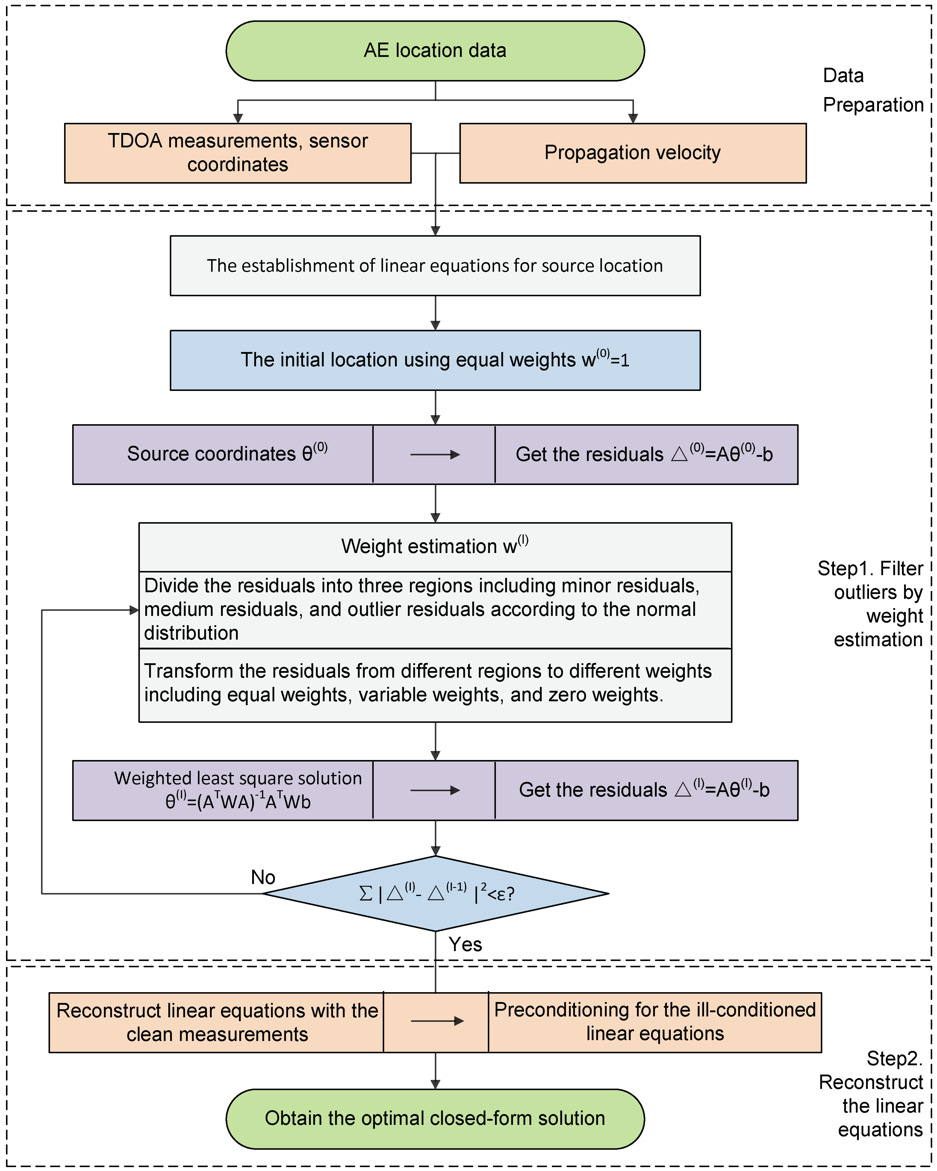
3.3. Location Process of Proposed Method

The whole procedures of PCFWE are shown in Figure 3 as below:
  • Establish linear equations for the source location.
  • Set index I = 0 and w i ( 0 ) = 1 for the primary iteration and obtain the initial location result θ ( 0 ) .
  • Calculate the residuals Δ ( 0 ) = A θ ( 0 ) b , which are used to generate the preliminary weights w i ( 1 ) according to Equation (7).
  • Conduct the next iteration, I = 1, and solve the weighted least squares solution θ ( 1 ) from Equation (14).
  • Update the weights w i ( 2 ) according to the residuals Δ ( 1 ) .
  • Use the new weights in the next location, where I = 2 and θ ( 2 ) is calculated.
  • Repeat the above calculations (steps 4–6) to optimize the weights and filter the outliers, until | Δ ( I ) Δ ( I 1 ) | 2 ε .
  • Reconstruct linear equations with the remaining measurements.
  • Precondition linear equations to lower the condition number and eliminate the ill condition.
  • Obtain the optimal closed-form solution by solving the preconditioned linear equations with Equation (18).

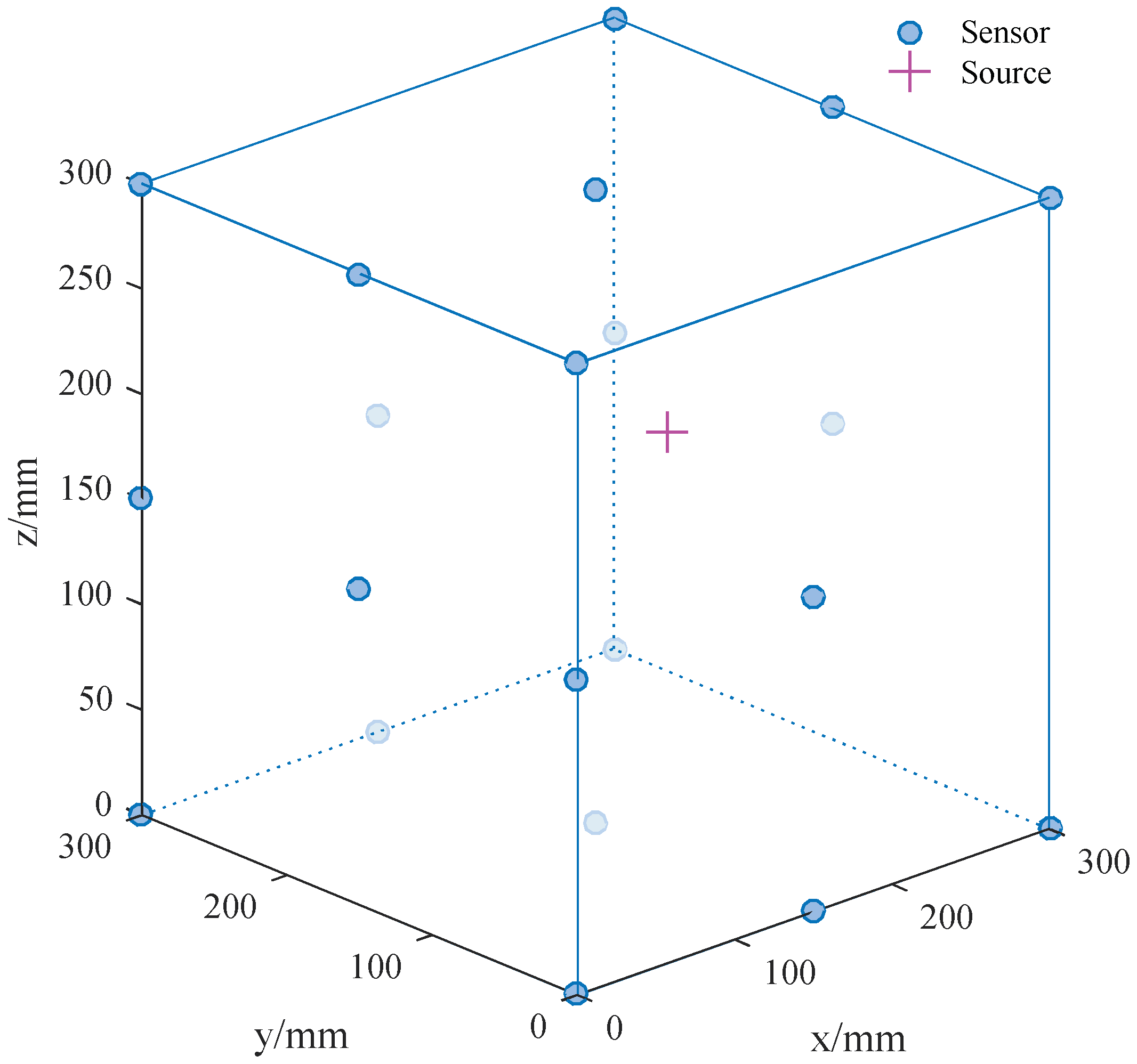
4. Experimental Verification

To verify the feasibility of this method, the AE source location experiment is carried out in this paper. The acoustic wave is collected by a DS5-16C Holographic Acoustic Emission Signal Analyzer (made by Beijing SoftLand Scientific and Technology Co., Ltd., Beijing, China). AE sources are generated by pencil-lead breaks. The HB pencil lead is 0.5 mm in diameter, and the pencil lead is broken at 30° on the surface of the specimen, according to the requirements of Metal Pressure Vessel Acoustic Emission Testing and Result Evaluation (GB/T181822000). The granite specimen that is 200 mm × 179 mm × 84 mm in size and an average velocity of 4600 m/s is used as a monitoring system. Sixteen RS-2A piezoelectric ceramic resonant sensors with the coordinates of (10, 10, 84), (190, 10, 84), (190, 170, 84), (12, 170, 84), (0, 80, 74), (110, 0, 74), (200, 80, 74), (90, 180, 74), (0, 170, 10), (0, 90, 10), (10, 0, 10), (100, 0, 10), (190, 0, 10), (200, 90, 10), (190, 180, 10), and (100, 180, 10) (in mm) respectively are mounted on the surface of the monitoring system. Sensors are numbered as Si (i = 0, 1, ···, 15) according to the arrival orders of the AE signals, and the nearest sensor S0 from the AE source is regarded as the reference sensor. Later, 15 TDOA measurements △ti (i = 1, 2, ···, 15) between the sensor pairs of S0 and Si are obtained. In addition, there are four AE sources generated by pencil-lead breaks, and their coordinates are P (80, 120, 84), Q (160, 60, 84), R (0, 120, 42), and T (120, 0, 42) respectively. Before signal acquisition, the voltage threshold of each channel is set as 10 mv, and the preamplifier gain is 40 dB.
Figure 4 shows the received AE waveforms by two sensors, in which t 0 and t 2 are the arrival times at sensor S0 and sensor S2, respectively. Then, TDOA measurement is formed by using the arrival times at the sensor pair S0 and S2, i.e., Δ t 2 = t 2 t 0 . The arrival times of the acoustic waves are picked manually according to the waveform diagram to ensure a high picking quality.

4.1. The Filtering of Outliers

TDOA measurements, the coordinates of triggered sensors, and average velocity are used to locate the four AE events by the method proposed in this paper. The outlier TDOA measurements are generated factitiously by adding ±30% large errors to the largest two measurements, which are used to simulate the picking deviation caused by automated programs in complex engineering practice. Location results with the additive outliers in measurements are determined by using the LLS method without the outliers filtering process, and the detailed data are listed in upper half of Table 1. It is clear to see that the location errors between the authentic coordinates and the location results are great, where the maximum absolute distance error reaches to 57.61 mm. Obviously, the location results are unreasonable and unreliable, because corrupted measurements dramatically affect the location accuracy. Therefore, it is significant to identify and filter the outliers for the AE source location.
Figure 5 illustrates the process of eliminating the outliers at the location of source T. The initial location using the LLS method with equal weights has a large location error due to the existence of the outliers shown in Step a. The corresponding residuals are obtained and shown in Step b; it can be seen that the absolute residuals of 1, 4, 5, 6, 7, 8, 9, 12, and 13 are less than the threshold λ m , so the corresponding weights of the measurements △t1, △t4, △t5, △t6, △t7, △t8, △t9, △t12, and △t13 are set as equal according to Equation (7), while the weights of the other measurements are set as 1 / Δ i . Moreover, it should be noted that no outliers can be found after the first location, because the residuals obtained by the initial location result can not reflect the deviations of the true model effectively, especially when outliers exist. Therefore, further iterations between the source location and weight estimation are necessary in order to filter the outliers, which are shown from step c to Step f. The 14th and 15th residuals exceed the maximum allowable deviation λ L at step c and d, respectively. Therefore, they are regarded as outliers, and △t14 and △t15 are considered outlier measurements that are filtered by setting the weights to zeros. The change of residuals between steps e and f is small enough, so the iteration stops. After that, linear equations are reconstructed by using the remaining measurements. Finally, the location results can be obtained by solving the new linear equations using the LLS method. It can be seen in Step g that the calculated result and theoretical locations respectively denoted by the diamond and spot are close to each other. Therefore, the location accuracy is improved effectively after outlier filtering.
The lower half of Table 1 lists the location results and absolute distance errors of the four AE sources after filtering the outliers. Through the comparison between location results before and after filtering the outliers in Figure 6, it is obvious that the location accuracy is improved significantly. For example, the absolute distance error of the source R is reduced to 9.28 mm from 57.61 mm, and the absolute distance error of source T is reduced to 10.55 mm from 46.82 mm. Therefore, it can be concluded that the location accuracy is improved effectively through the filtering of outliers. However, it should be noticed that linear equations are always in or near ill condition, which still cause a large deviation with a minor disturbance in the coefficient. Location accuracy is improved using a preconditioning method by reducing the ill condition of linear equations. Location results in the following section, Section 4.2, prove the ability of solving source coordinates with higher accuracy by preconditioning for linear equations.

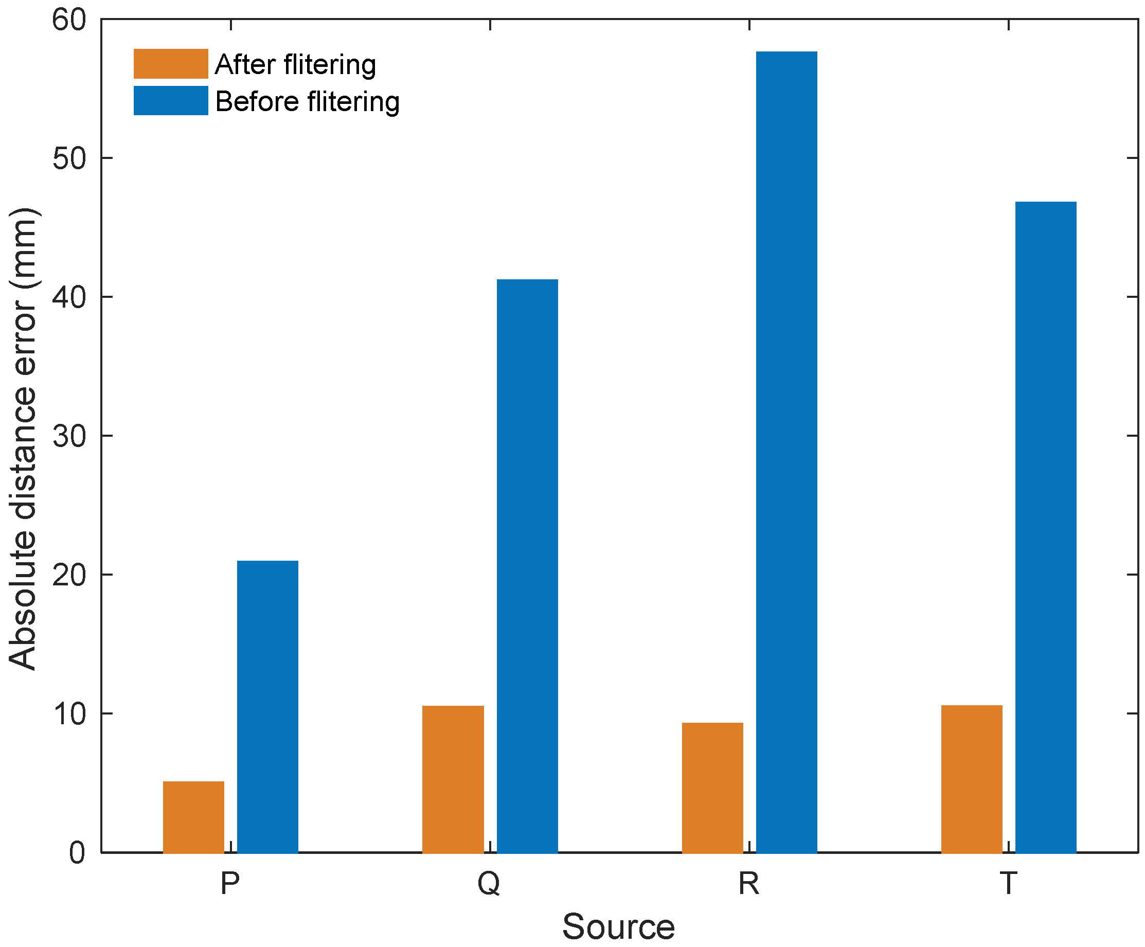
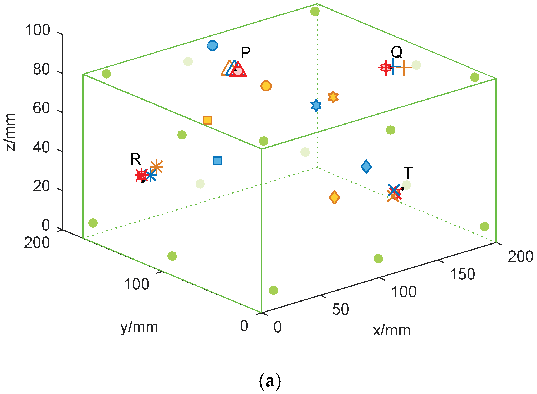
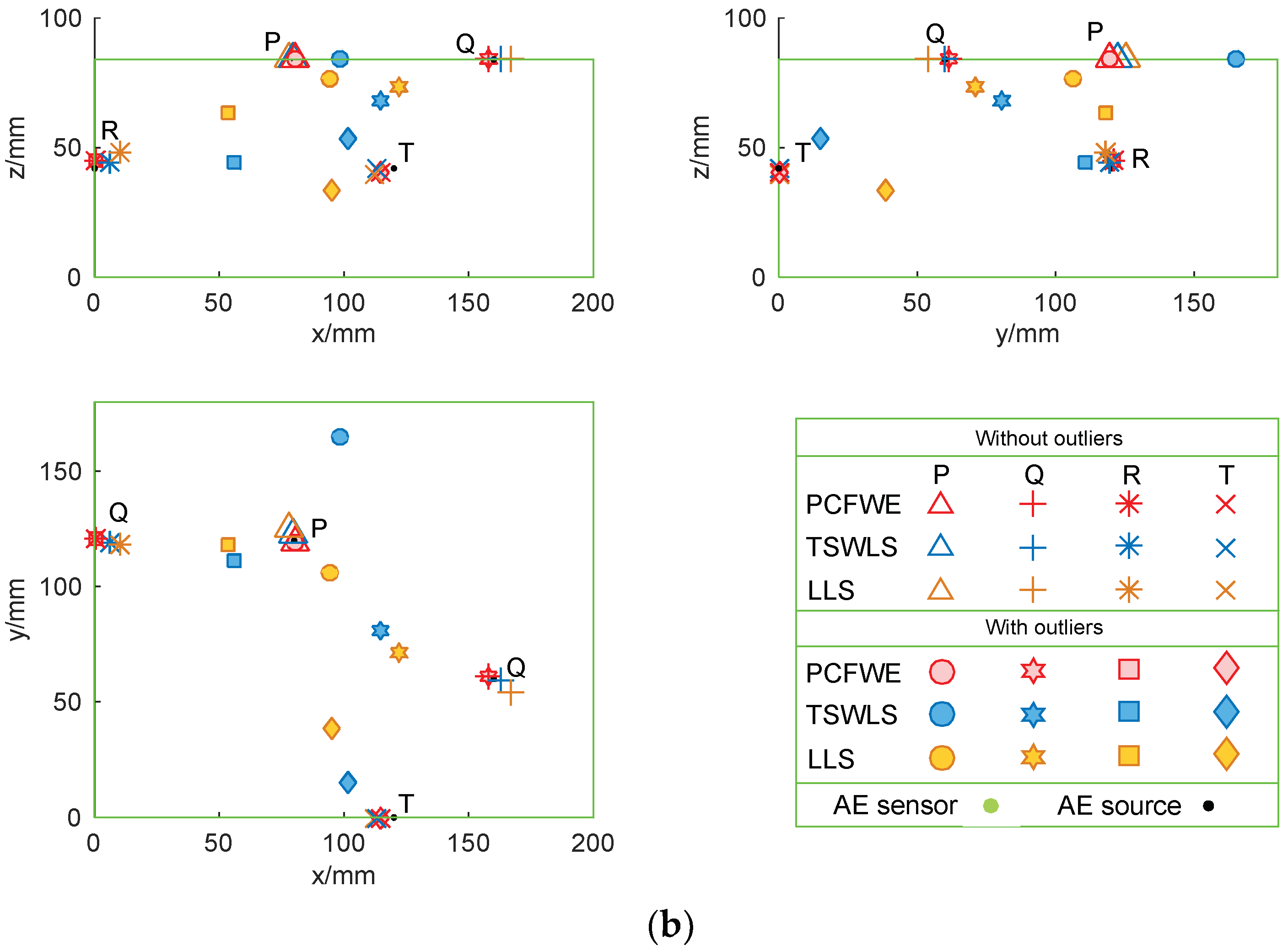
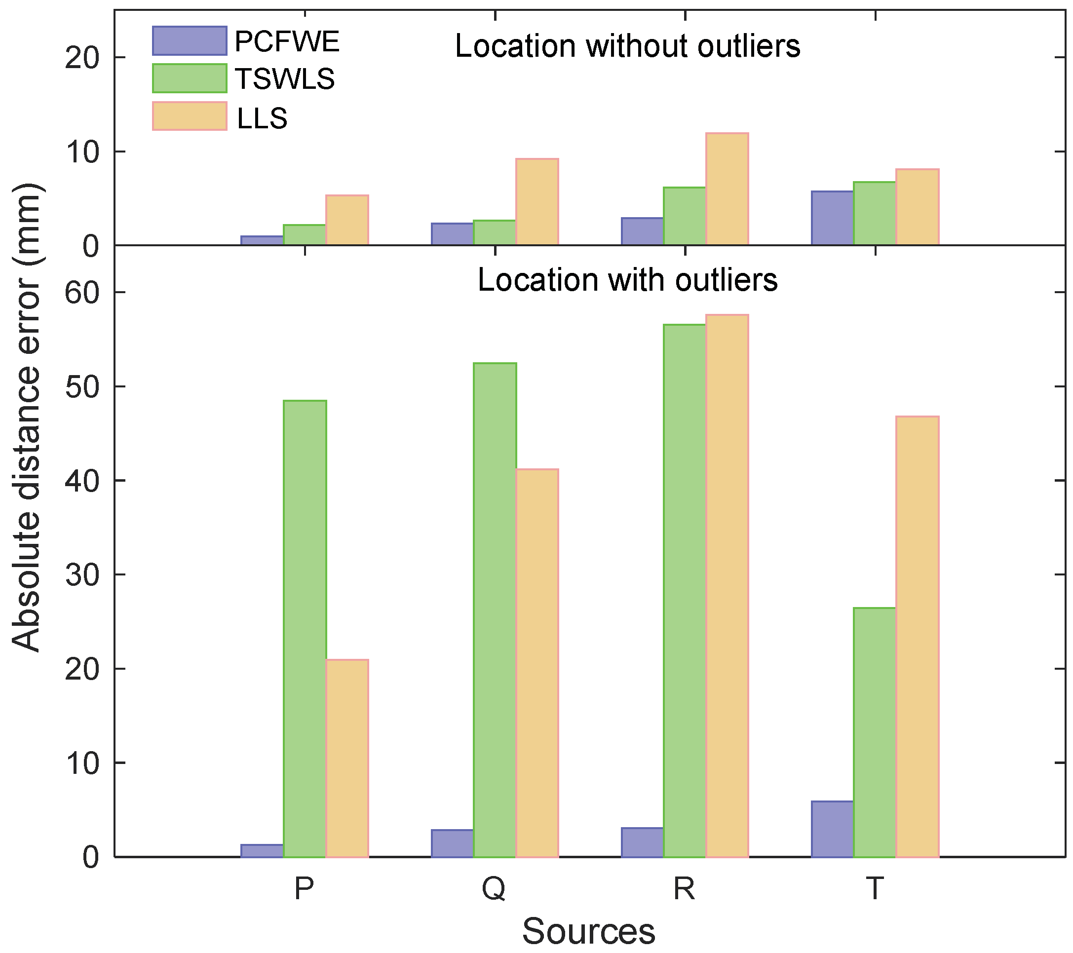
4.2. Comparing Location Results with and without Outliers

For each event, the mentioned TSWLS and LLS methods in Section 1 and Section 2 are applied for comparison with the PCFWE with additive outliers and without additive outliers.
Figure 7 shows the location results in a three-dimensional space. It can be seen that the location results of the PCFWE method are approximate to the true sources, regardless of whether the additive outliers are contained in the TDOA measurements or not. Location results, which are determined by the TSWLS and LLS methods, also achieve desirable location results with minor deviations from true sources, but it deviates dramatically if outliers exist. Figure 8 shows the absolute distance errors of location results for three methods with and without outliers. When there are no outliers in the measurements, the absolute distance errors of the three methods are all small, while the PCFWE is the smallest, because of the applied preconditioning method. When the outliers are contained in measurements, the location errors of the traditional methods are dramatically large, while the location performance of the proposed method always remains stable with a higher location accuracy.
From Table 2, it is obvious that the biggest absolute distance errors of traditional methods can occasionally exceed 50 mm. There are two main reasons for the poor location results of traditional methods. Firstly, due to the influence of an outlier in the measurement, residuals are significantly intensified by the least squares principle, which results in a large deviation to the final location result for traditional methods. Secondly, traditional methods take no account of the problem of ill-conditioned linear equations, which also affect the location accuracy to some extent. It is worth mentioning that the proposed method in this paper can achieve an accurate location, where the best absolute distance error can reach about 1 mm. The good performance of the new method is attributed to the fact that, it not only reduces the ill condition of linear equations, it also eliminates outliers. Therefore, location accuracy is improved effectively.

5. Conclusions and Discussion

Considering that the outliers in the complex engineering environment have a serious effect on the location performance, the PCFWE method is proposed to improve the location accuracy in this paper. Firstly, the weight estimation is developed by transforming residuals to weights according to normal distribution. Updated weights are incorporated into the source location to provide a weighted least squares solution. Then, outliers are filtered by iterating between the weight estimation and source location. Linear equations, which are reconstructed with remaining measurements after filtering outliers, are ill-conditioned and need to be preconditioned to lower the condition number. Finally, the optimal source coordinates can be obtained by solving preconditioned linear equations. The proposed location method is verified by the experiment of pencil-lead breaks; the results show that the proposed PCFWE method achieves a stable and accurate location both with outliers and without outliers in measurements. However, how many outliers the proposed method can tolerate, and the sensitivity of the wave velocity, still need further investigation.

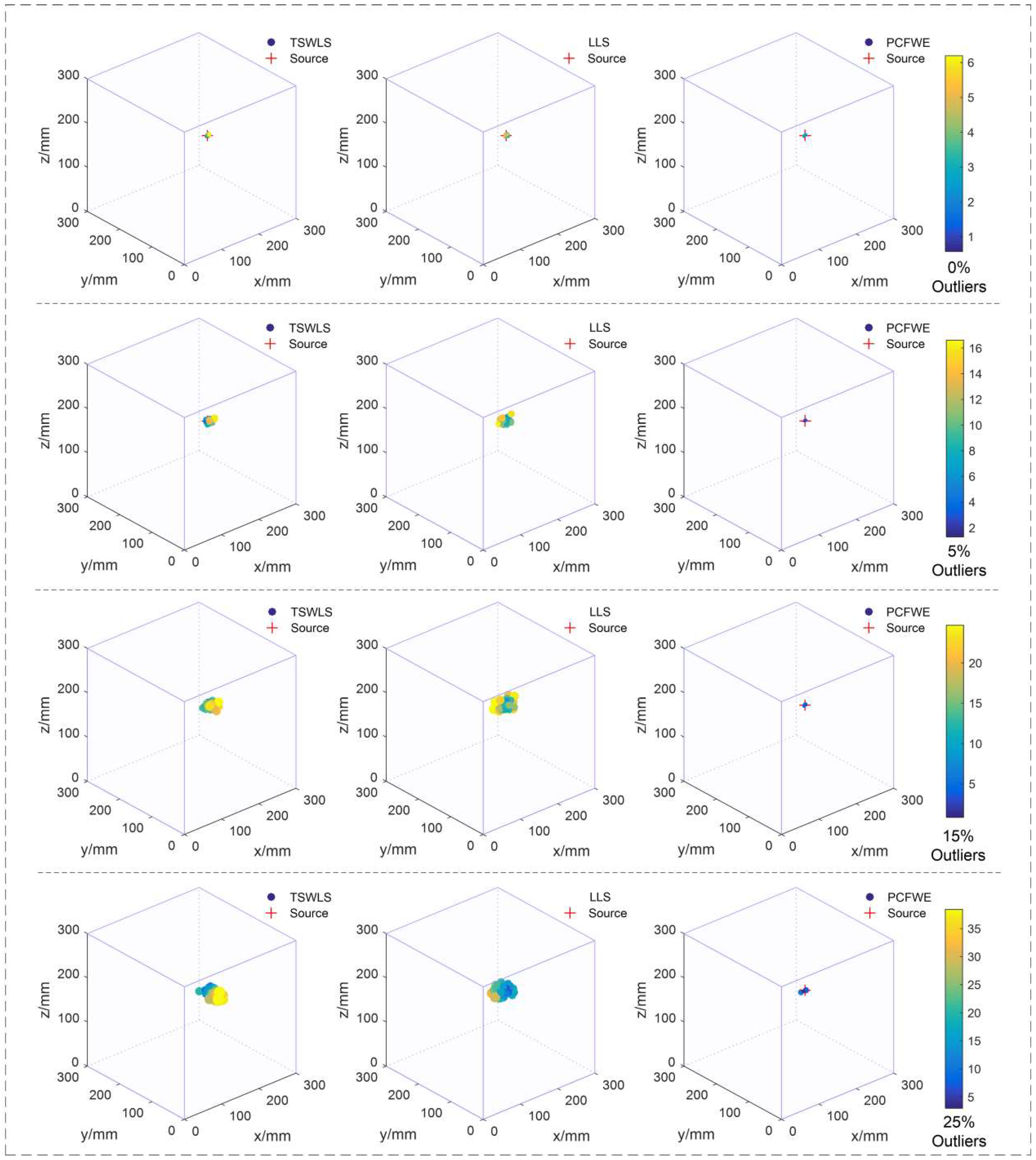
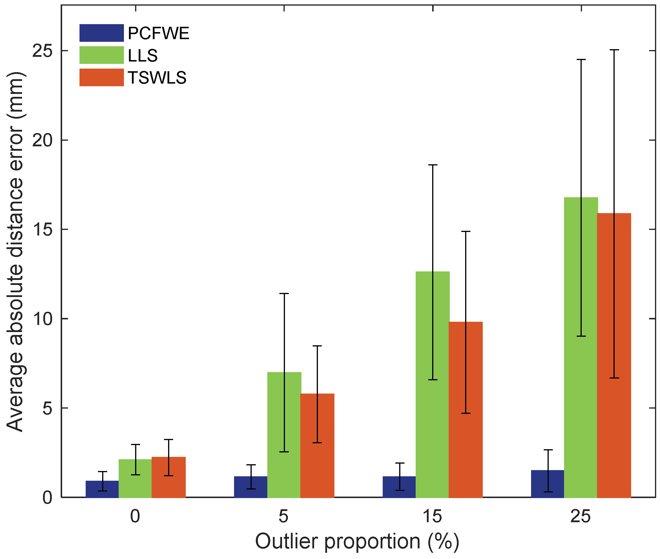
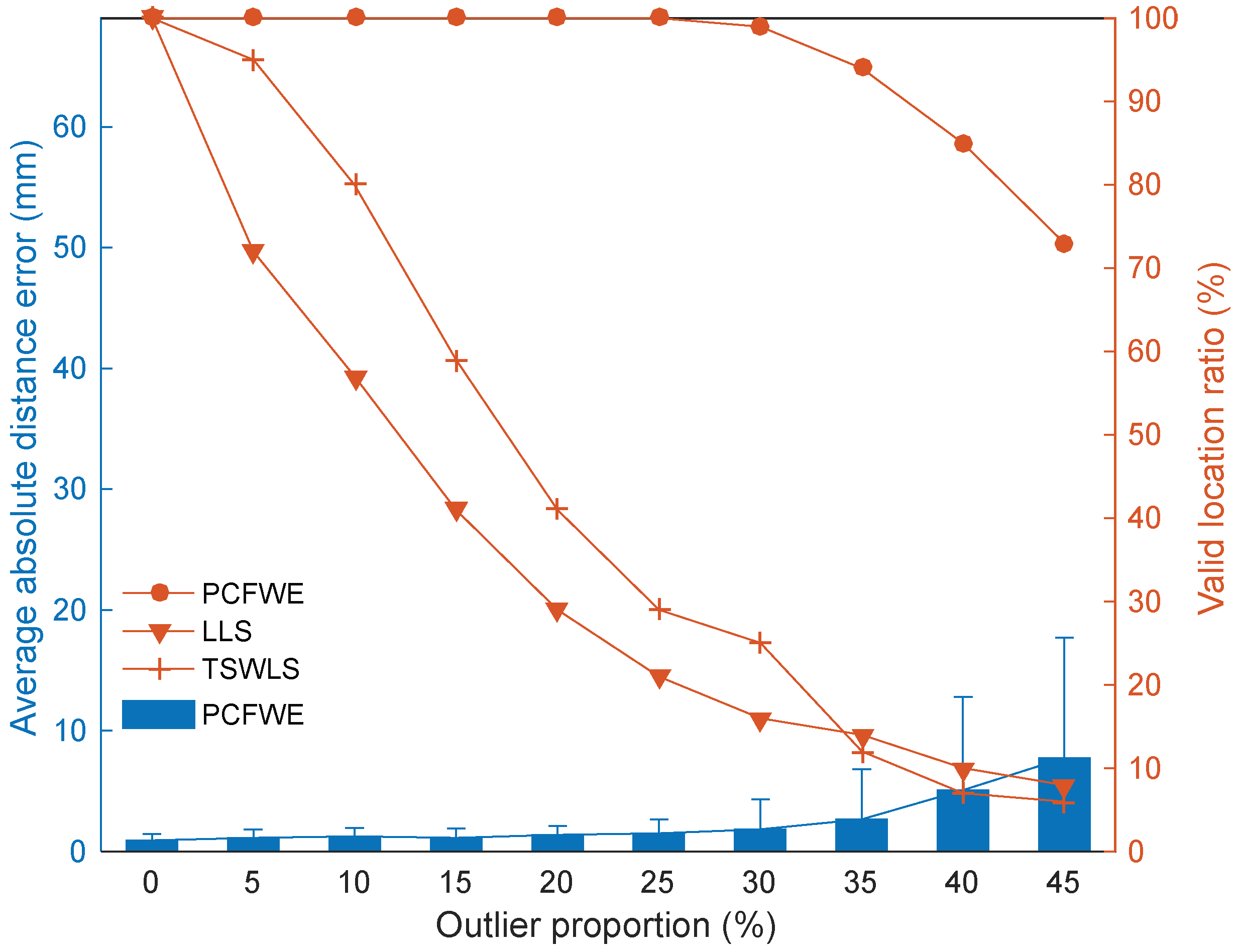
5.1. Outlier Tolerance

To investigate the outlier-tolerant ability of PCFWE under different outlier proportions, simulating tests are used because of the admirable repeatability and flexibility. Simulating tests with controllable errors in the input data such as TDOA measurements and the velocity system are described in this section. Figure 9 shows an assumed cubic locating system with a side length of 300 mm, where an AE source O (150, 100, 200) surrounded by 21 sensors is set to generate AE signals. It is assumed that the trigger time is 0 μs, and the average wave velocity of the media is 5000 m/s. In addition, to simulate minor systemic errors in TDOA measurements, the extra random errors from the normal distribution with a mean of zero and a standard deviation of 2% of measurements are added. To simulate the uncertainty of the velocity along different paths, a minor error of 5% of velocity for each path is generated. For measurements with abnormal errors (outliers), dramatic errors of ±30% of TDOA measurements, which are much larger than the systemic error, are added with different proportions. Thus, the simulated location consists of velocity uncertainty, systemic minor errors, and different outlier proportions.
To obtain a reliable statistical result, the AE source location is repeated 100 times by random changes of TDOA measurements and the velocity errors, and then their location coordinates are calculated. The location results of the 100 simulating tests with different outlier proportions are shown in Figure 10. It can be seen that all of the sizes of solid circles are small and close to true sources, when there is no outlier in the input data. However, they have obvious differences as shown in Figure 11, where the average absolute distance error of the PCFWE is smaller than that of traditional methods, due to the use of preconditioning for the linear equations. In other words, the PCFWE performs better than traditional location methods without outliers. The location performance of the PCFWE differs more substantially from traditional methods in the presence of outliers. Solid circles of traditional methods always appear more discrete and have a larger diameter with the increase of outlier proportions, which indicates that the location errors increase with outlier proportions. While the solid circles of the PCFWE always appear more compact and darker under different outlier proportions, which illustrate the PCFWE location method has a higher accuracy and stability than traditional methods.
Figure 11 shows the average absolute distance errors of 100 location results under different outlier proportions determined by three methods. The average absolute distance errors for traditional methods increase dramatically with the increasing of outlier proportions. Whereas, the average absolute distance errors of PCFWE method always keep low and stable under different outlier proportions, due to the filtering of outliers in calculation, which further illustrates the good performance of the PCFWE method.
Moreover, the relationship between valid location ratios and outlier proportions is displayed in Figure 12. The valid location ratio is the location proportion whose location errors are smaller than 2% of the distance between the two farthest sensors in the sensor array. Clearly, the two curves of traditional methods decline dramatically with the increase of outliers, the valid locations of which are less than 30% when there are 25% outliers. Compared with traditional methods, the curve of the PCFWE always keeps stable and achieves valid locations of nearly 100% when the outliers are less than or equal to 25%. Then, the curve falls to 73% at the outlier proportion of 45%, which is still far above the other two curves that have valid locations of less than 10%.
Therefore, the outlier-tolerant ability of the proposed method is far higher than those of traditional methods, which can realize valid locations of more than 90%, even when the outlier proportion reaches 35%. Therefore, the proposed method is suitable for engineering practice where the outliers commonly exist. In addition, when there are too many outliers (more than 35%), the PCFWE method gives a warning to check the environment noise or equipment malfunctions.

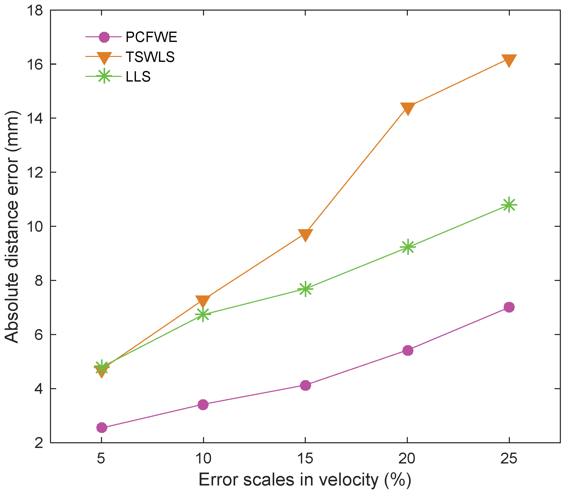
5.2. Velocity Sensibility

The premeasured velocity is necessary for most location methods, and measurement errors in velocity are unavoidable due to the complex construction environment and manual operation. Moreover, the wave velocity of the propagation medium always changes with material testing or engineering construction. An effective location method should have a lower velocity sensitivity, i.e., a higher tolerance of velocity error. Therefore, the analysis of the velocity sensitivity of different methods is conducted in this section. This simulating test is still based on the above location system. To obtain a reliable statistical result, 100 AE sources are selected randomly inside the sensor array to generate AE signals. Besides, the 2% minor systemic errors in measurements are applied to simulate minor systemic errors, and 5% to 25% errors are added to velocity, in turn to investigate the velocity sensitivity. Hence, the simulated location consists of systemic minor errors in TDOA measurements and different error scales in velocity.
The average absolute distance errors under different error scales in velocity are calculated, which are shown in Figure 13. All three curves show a rising trend with the increase of error scales in velocity, but the curve of the PCFWE is significantly lower than the other two methods. Therefore, the PCFWE has the lowest velocity sensitivity, which indicates that the PCFWE can bear larger errors in velocity than traditional methods.
During material testing, the wave velocity changes with the loading stress. Through the analysis of the velocity sensitivity of different methods, conclusions are gained, as the proposed method has a stronger tolerance to velocity errors, which is suitable for a material test where the wave velocity changes along with the test. However, in the later stage of a test, the wave velocity changes dramatically due to the propagation of cracks and voids. The proposed method also fails to achieve an ideal location result. A possible solution is the dynamic inversion for real-time wave velocity by taking the velocity as an unknown parameter or modifying the velocity data according to the real-time velocity test, which still needs to be investigated in future research [46].
In practical engineering applications, the proposed method still has the following two limitations. This method is established based on a uniform medium, while most of the materials in engineering practice are anisotropic and heterogeneous, such as rock and concrete. In addition, although the sensitivity of the wave velocity is low, the proposed method is still affected by the velocity error. Besides, it is troublesome to measure the wave velocity in advance or real-time. Therefore, further studies should extend the method to address these issues.

Author Contributions

Z.Z. and Y.R. proposed the location method and performed the experiments; Z.Z., Y.R., J.Z. and R.C. analysed the data and wrote the paper; and L.D., L.C. and X.C. supervised the research and revised the manuscript.

Acknowledgments

The authors would like to acknowledge financial support from the National Basic Research Program of China (973 Program) (No. 2015CB060200), the National Natural Science Foundation of China (Nos. 41772313 and 51478479), and the Fundamental Research Funds for the Central Universities of Central South University (No. 2018zzts716).

Conflicts of Interest

The authors declare no conflict of interest.

Abbreviations

The following abbreviations are used in this manuscript:
AEAcoustic Emission
PCFWEPreconditioned closed-form solution based on weight estimation
TDOATime difference of arrival
TSWLSTwo-step weighted least squares
LLSLinear least squares

References

  1. Dworakowski, Z.; Kohut, P.; Gallina, A.; Holak, K.; Uhl, T. Vision-based algorithms for damage detection and localization in structural health monitoring. Struct. Control Health 2016, 23, 35–50. [Google Scholar] [CrossRef]
  2. Topolář, L.; Pazdera, L.; Kucharczyková, B.; Smutný, J.; Mikulášek, K. Using acoustic emission methods to monitor cement composites during setting and hardening. Appl. Sci. 2017, 7, 451. [Google Scholar] [CrossRef]
  3. Muñoz, C.G.; Márquez, F.G. A new fault location approach for acoustic emission techniques in wind turbines. Energies 2016, 9, 40. [Google Scholar] [CrossRef]
  4. Martini, A.; Troncossi, M.; Rivola, A. Leak detection in water-filled small-diameter polyethylene pipes by means of acoustic emission measurements. Appl. Sci. 2016, 7, 2. [Google Scholar] [CrossRef]
  5. Zhou, Z.L.; Cai, X.; Ma, D.; Cao, W.Z.; Chen, L.; Zhou, J. Effects of water content on fracture and mechanical behavior of sandstone with a low clay mineral content. Eng. Fract. Mech. 2018, 193, 47–65. [Google Scholar] [CrossRef]
  6. Dong, L.J.; Sun, D.Y.; Li, X.B.; Du, K. Theoretical and Experimental Studies of Localization Methodology for AE and Microseismic Sources without Pre-Measured Wave Velocity in Mines. IEEE Access 2017, 5, 16818–16828. [Google Scholar] [CrossRef]
  7. Lacidogna, G.; Piana, G.; Carpinteri, A. Acoustic Emission and Modal Frequency Variation in Concrete Specimens under Four-Point Bending. Appl. Sci. 2017, 7, 339. [Google Scholar] [CrossRef]
  8. Li, X.; Deng, Z.D.; Rauchenstein, L.T.; Carlson, T.J. Contributed review: Source-localization algorithms and applications using time of arrival and time difference of arrival measurements. Rev. Sci. Instrum. 2016, 87, 921–960. [Google Scholar] [CrossRef] [PubMed]
  9. Huang, Y.; Benesty, J.; Elko, G.W.; Mersereati, R.M. Real-time passive source localization: A practical linear-correction least-squares approach. IEEE Trans. Speech Audio Process. 2001, 9, 943–956. [Google Scholar] [CrossRef]
  10. Roberts, R.G.; Christoffersson, A.; Cassidy, F. Real-time event detection, phase identification and source location estimation using single station three-component seismic data. Geophys. J. Int. 2010, 97, 471–480. [Google Scholar] [CrossRef]
  11. Al-Jumaili, S.K.; Pearson, M.R.; Holford, K.M.; Eaton, M.J.; Pullin, R. Acoustic emission source location in complex structures using full automatic delta t mapping technique. Mech. Syst. Signal Process. 2016, 72–73, 513–524. [Google Scholar] [CrossRef]
  12. Dong, L.J.; Shu, W.W.; Han, G.J.; Li, X.L.; Wang, J. A Multi-Step Source Localization Method With Narrowing Velocity Interval of Cyber-Physical Systems in Buildings. IEEE Access 2017, 5, 20207–20219. [Google Scholar] [CrossRef]
  13. Mostafapour, A.; Davoodi, S. Acoustic emission source locating in two-layer plate using wavelet packet decomposition and wavelet-based optimized residual complexity. Struct. Control. Health 2017. [Google Scholar] [CrossRef]
  14. Kundu, T. Acoustic source localization. Ultrasonics 2014, 54, 25–38. [Google Scholar] [CrossRef] [PubMed]
  15. Schau, H.; Robinson, A. Passive source location employing spherical surfaces from time-of-arrival differences. IEEE Trans. Aerosp. Electron. Syst. 1987, 35, 1223–1225. [Google Scholar]
  16. Smith, J.O.; Abel, J.S. Closed-form least-squares source location estimation from range-difference measurements. IEEE Trans. Acoust. Speech Signal Process. 1987, 35, 1661–1669. [Google Scholar] [CrossRef]
  17. Zhou, Z.L.; Rui, Y.C.; Zhou, J.; Dong, L.J.; Cai, X. Locating an acoustic emission source in multilayered media based on the refraction path method. IEEE Access 2018. [Google Scholar] [CrossRef]
  18. Zhou, Z.L.; Zhou, J.; Dong, L.J.; Cai, X.; Rui, Y.C.; Ke, C.T. Experimental study on the location of an acoustic emission source considering refraction in different media. Sci. Rep. 2017, 7, 7472. [Google Scholar] [CrossRef] [PubMed]
  19. Drew, J.; White, R.S.; Tilmann, F.; Tarasewicz, J. Coalescence microseismic mapping. Geophys. J. Int. 2013, 195, 1773–1785. [Google Scholar] [CrossRef] [Green Version]
  20. Enosh, I.; Weiss, A.J. Outlier identification for toa-based source localization in the presence of noise. Signal Process. 2014, 102, 85–95. [Google Scholar] [CrossRef]
  21. Allen, R.V. Automatic earthquake recognition and timing from single traces. Bull. Seismol. Soc. Am. 1978, 68, 1521–1532. [Google Scholar]
  22. Kuperkoch, L.; Meier, T.; Lee, J.; Friederich, W.; Grp, E.W. Automated determination of P-phase arrival times at regional and local distances using higher order statistics. Geophys. J. Int. 2010, 181, 1159–1170. [Google Scholar] [CrossRef]
  23. Niccolini, G.; Xu, J.; Manuello, A.; Lacidogna, G.; Carpinteri, A. Onset time determination of acoustic and electromagnetic emission during rock fracture. Prog. Electromagn. Res. Lett. 2012, 35, 51–62. [Google Scholar] [CrossRef]
  24. Akaike, H. A new look at the statistical model identification. Trans. Autom. Control 1974, 19, 716–723. [Google Scholar] [CrossRef]
  25. Ge, M.C. Efficient mine microseismic monitoring. Int. J. Coal Geol. 2005, 64, 44–56. [Google Scholar] [CrossRef]
  26. Dong, L.J.; Li, X.B.; Ma, J.; Tang, L.Z. Three-dimensional analytical comprehensive solutions for acoustic emission/microseismic sources of unknown velocity system. Chin. J. Rock Mech. Eng. 2017, 36, 186–197. [Google Scholar]
  27. Taghizadeh, M.J.; Haghighatshoar, S.; Asaei, A.; Garner, P.N.; Bourlard, H. Robust microphone placement for source localization from noisy distance measurements. In Proceedings of the IEEE International Conference on Acoustics, Speech and Signal Processing (ICASSP), Brisbane, QLD, Australia, 19–24 April 2015; pp. 2579–2583. [Google Scholar]
  28. Picard, J.S.; Weiss, A.J. Time difference localization in the presence of outliers. Signal Process. 2012, 92, 2432–2443. [Google Scholar] [CrossRef]
  29. Li, P.; Ma, X. Robust acoustic source localization with TDOA based RANSAC algorithm. In Proceedings of the 5th International Conference on Intelligent Computing (ICIC), Ulsan, Korea, 16–19 September 2009; pp. 222–227. [Google Scholar]
  30. Weng, Y.; Xiao, W.D.; Xie, L.H. Total least squares method for robust source localization in sensor networks using tdoa measurements. Int. J. Distrib. Sens. Netw. 2011, 7, 172902. [Google Scholar] [CrossRef]
  31. Lin, L.; So, H.C.; Chan, F.K.W.; Chan, Y.T.; Ho, K.C. A new constrained weighted least squares algorithm for tdoa-based localization. Signal Process. 2013, 93, 2872–2878. [Google Scholar] [CrossRef]
  32. Mensing, C.; Plass, S. Positioning algorithms for cellular networks using TDOA. In Proceedings of the IEEE International Conference on Acoustics, Speech and Signal Processing (ICASSP), Toulouse, France, 14–19 May 2006; pp. 513–516. [Google Scholar]
  33. Chan, Y.T.; Hang, H.Y.C.; Ching, P.C. Exact and approximate maximum likelihood localization algorithms. IEEE Trans. Veh. Technol. 2006, 55, 10–16. [Google Scholar] [CrossRef]
  34. Chen, J.C.; Hudson, R.E.; Yao, K. Maximum-likelihood source localization and unknown sensor location estimation for wideband signals in the near-field. IEEE Trans. Signal Proces. 2002, 50, 1843–1854. [Google Scholar] [CrossRef]
  35. Jiang, Y.; Azimi-Sadjadi, M.R. A Robust Source Localization Algorithm Applied to Acoustic Sensor Network. In Proceedings of the IEEE International Conference on Acoustics, Speech and Signal Processing (ICASSP), Honolulu, HI, USA, 15–20 April 2007; pp. 1233–1236. [Google Scholar]
  36. Li, X.B.; Wang, Z.W.; Dong, L.J. Locating single-point sources from arrival times containing large picking errors (lpes): The virtual field optimization method (vfom). Sci. Rep. 2016, 6, 19205. [Google Scholar] [CrossRef] [PubMed]
  37. Li, N.; Wang, E.Y.; Sun, Z.Y.; Li, B.L. Simplex microseismic source location method based on l1 norm statistical standard. J. China Coal Soc. 2014, 39, 2431–2438. [Google Scholar]
  38. Prugger, A.F.; Gendzwill, D.J. Microearthquake location: A nonlinear approach that makes use of a simplex stepping procedure. Bull. Seismol. Soc. Am. 1988, 78, 799–815. [Google Scholar]
  39. Ciampa, F.; Meo, M. Acoustic emission source localization and velocity determination of the fundamental mode A0 using wavelet analysis and a Newton-based optimization technique. Smart Mater. Struct. 2010, 19, 045027. [Google Scholar] [CrossRef]
  40. Foy, W.H. Position-location solutions by taylor-series estimation. IEEE Trans. Aerosp. Electron. Syst. 2007, AES-12, 187–194. [Google Scholar] [CrossRef]
  41. Chan, Y.T.; Ho, K.C. A simple and efficient estimator for hyperbolic location. IEEE Trans. Signal Process. 1994, 42, 1905–1915. [Google Scholar] [CrossRef]
  42. Ho, K.C.; Xu, W. An accurate algebraic solution for moving source location using TDOA and FDOA measurements. IEEE Trans. Signal Process. 2004, 52, 2453–2463. [Google Scholar] [CrossRef]
  43. Ho, K.C. Bias reduction for an explicit solution of source localization using TDOA. IEEE Trans. Signal Process. 2012, 60, 2101–2114. [Google Scholar] [CrossRef]
  44. Ho, K.C.; Lu, X.; Kovavisaruch, L.O. Source localization using TDOA and FDOA measurements in the presence of receiver location errors: Analysis and solution. IEEE Trans. Signal Process. 2007, 55, 684–696. [Google Scholar] [CrossRef]
  45. Xu, B.; Qi, W.D.; Wei, L.; Liu, P. Turbo-TSWLS: Enhanced two-step weighted least squares estimator for TDOA-based localisation. Electron. Lett. 2012, 48, 1597–1598. [Google Scholar] [CrossRef]
  46. Dong, L.J.; Shu, W.W.; Li, X.B.; Han, G.J.; Zou, W. Three dimensional comprehensive analytical solutions for locating sources of sensor networks in unknown velocity mining system. IEEE Access 2017, 5, 11337–11351. [Google Scholar] [CrossRef]
  47. Dong, L.J.; Zou, W.; Li, X.B.; Shu, W.W.; Wang, Z.W. Collaborative localization method using analytical and iterative solutions for microseismic/acoustic emission sources in the rockmass structure for underground mining. Eng. Fract. Mech. 2018. [Google Scholar] [CrossRef]
  48. Leighton, F.; Duvall, W.I. Least Squares Method for Improving Rock Noise Source Location Techniques; USBM RI 7626; Bureau of Mines: Washington, DC, USA, 1972; pp. 26–69.
  49. Fang, W.H.; Liu, L.C.; Yang, J.P.; Shui, A.S. A non-iterative ae source localization algorithm with unknown velocity. J. Log. Eng. Univ. 2016, 32, 1–7. [Google Scholar]
  50. Li, X.B.; Dong, L.J. An efficient closed-form solution for acoustic emission source location in three-dimensional structures. AIP Adv. 2014, 4, 152–160. [Google Scholar] [CrossRef]
  51. Dong, L.J.; Li, X.B.; Xie, G.N. An analytical solution for acoustic emission source location for known P wave velocity system. Math. Probl. Eng. 2014, 2014, 290686. [Google Scholar] [CrossRef]
  52. Strutz, T. Data Fitting and Uncertainty: A Practical Introduction to Weighted Least Squares and Beyond; Vieweg and Teubner Verlag: Wiesbaden, Germany, 2010. [Google Scholar]
  53. Chauvenet, W. A Manual of Spherical and Practical Astronomy, 4th ed.; J.B. Lippincott Co.: Philadelphia, PA, USA, 1871; pp. 558–568. [Google Scholar]
  54. Holland, P.W.; Welsch, R.E. Robust regression using iteratively reweighted least-squares. Commun. Stat. Theory Mothods 1977, 6, 813–827. [Google Scholar] [CrossRef]
Figure 1. Residual division according to the normal distribution. In this figure, PDF is the normal probability density function and CDF means the cumulative distribution function.
Applsci 08 00949 g001
Figure 2. Change of weights with the increasing absolute residuals and the probability of the absolute residuals less than kσ (|△| < kσ).
Applsci 08 00949 g002
Figure 3. Flow charts of preconditioned closed-form solution based on weight estimation (PCFWE) method location process.
Applsci 08 00949 g003
Figure 4. Acoustic emission (AE) signals and arrival times at different sensors.
Applsci 08 00949 g004
Figure 5. The process of locating the AE source T using the PCFWE method. The weights in this figure have been standardized by wi/sum(wi).
Applsci 08 00949 g005
Figure 6. Comparison of location errors before and after filtering using the LLS method.
Applsci 08 00949 g006
Figure 7. Location results from three methods: (a) three-dimensional (3D) schematic diagram of location results and sensor layout; (b) projections of AE events on the x-z, y-z, and x-y planes.
Applsci 08 00949 g007aApplsci 08 00949 g007b
Figure 8. The absolute distance error of the location results for three methods.
Applsci 08 00949 g008
Figure 9. Layout of sensors and location of the AE source.
Applsci 08 00949 g009
Figure 10. Three-dimensional location maps determined by three methods with outlier proportions of 0%, 5%, 15%, and 25% respectively. Diameters of solid circles indicate the location error, and smaller diameters indicate a higher location accuracy. To further distinguish the location accuracy of different sources, colors in the solid circles also indicate the location accuracy in millimeters.
Applsci 08 00949 g010
Figure 11. The average absolute errors of the AE sources determined by three methods under different outlier proportions.
Applsci 08 00949 g011
Figure 12. Valid location ratios of three methods and the average location error of the PCFWE under different outlier proportions.
Applsci 08 00949 g012
Figure 13. The average absolute distance error determined using three methods under different error scales in velocity.
Applsci 08 00949 g013
Table 1. Closed-form solutions before and after filtering using the linear least squares (LLS) method.
SourcesTrue Source CoordinatesLocation ResultsAbsolute Distance Error (mm)
x (mm)y (mm)z (mm)x (mm)y (mm)z (mm)
Without filteringP80.00120.0084.0093.94106.2076.6020.96
Q160.0060.0084.00121.7171.0273.4541.21
R0.00120.0042.0053.29117.8863.7857.61
T120.000.0042.0095.2538.8733.7346.82
filteringP80.00120.0084.0078.14124.7184.005.07
Q160.0060.0084.00168.6654.0484.0010.51
R0.00120.0042.007.82119.3346.969.28
T120.000.0042.00111.220.0036.1510.55
Table 2. Coordinates of AE sources solved by three methods.
AE SourceOutliersPCFWETSWLSLLS
x (mm)y (mm)z (mm)Absolute Distance Error (mm)x (mm)y (mm)z (mm)Absolute Distance Error (mm)x (mm)y (mm)z (mm)Absolute Distance Error (mm)
PNo80.46119.1284.000.9979.96122.1884.002.1877.98124.9784.005.37
Yes80.60118.8684.001.2998.24164.9484.0048.5093.94106.2076.6020.96
QNo158.0861.4084.002.38162.6559.5784.002.69167.0654.1184.009.20
Yes157.8061.8884.002.89114.4580.8068.2352.50121.7171.0273.4541.21
RNo0.00121.0844.752.965.78119.3644.056.1710.11117.7947.9311.93
Yes0.00121.2444.813.0755.81110.8244.0856.6053.29117.8863.7857.61
TNo114.430.0040.535.76113.240.0042.306.76112.170.0039.888.12
Yes114.280.0040.555.90101.3814.8253.5626.4695.2538.8733.7346.82

