Article

Online Dynamic Balance Technology for High Speed Spindle Based on Gain Parameter Adaption and Scheduling Control

College of Mechanical Engineering, Tianjin University of Technology and Education, Tianjin 300222, China
*
Author to whom correspondence should be addressed.
Appl. Sci. 2018, 8(6), 917; https://doi.org/10.3390/app8060917
Submission received: 13 April 2018 / Revised: 5 May 2018 / Accepted: 21 May 2018 / Published: 3 June 2018
(This article belongs to the Section Mechanical Engineering)

Abstract

:
Unbalance vibration is one of the main vibration forms of a high speed machine tool spindle. The overlarge unbalance vibration will have some adverse effects on the working life of the spindle system and the surface quality of the work-piece. In order to reduce the unbalance of a high speed spindle system, a pneumatic online dynamic balance device and its control system are presented in the paper. To improve the balance accuracy and adaptation of the balance system, the gain parameter adaption and scheduling control method are proposed first, and then the different balance effects of the influence coefficient method and the gain scheduling control method are compared through many dynamic balance experiments of the high speed spindle. The experimental results indicate that the gain parameters can be changed timely according to the transformation of the speed and kinetic parameters of the spindle system. The balance accuracy can be improved for a high speed spindle with time-varying characteristics, based on the adaptive gain scheduling control method.

1. Introduction

Online balance technology is the ideal vibration suppression method for the spindle system of a high speed and high precision machine tool. Usually, the online balance system consists of a balance device, signal testing, and a control system. For the online control method, many new online dynamic methods have been proposed in recent years. For example, D.Y. Jung et al. developed a new hybrid imbalance vibration control approach for an auto-balancer device (ABD) rotor system supported by a normal passive bearing augmented with an active magnetic bearings (AMB) to enhance the balancing and vibration isolation capabilities [1]. M. Xiang et al. proposed an auto balancing control scheme using adaptive feed-forward compensation based on a least mean square (LMS) algorithm. In this LMS algorithm, the two input signals were synchronous displacement and their orthogonal signals [2]. S.Q. Zheng explored a novel auto balancing method for a magnetically suspended rotor in a motor driveline system based on synchronous rotating frame (SRF) transformation [3].
In general, the typical methods of online balance control for the rotor are the influence coefficient method and the gain scheduling control method or their composition. In 1996, based on the influence coefficient method and graphic vector composition, W.H. Choi et al. presented a calculating method of optimum correction mass within permissible vibration limits for rotating machinery in two-plane field balancing. A genetic algorithm was used for vector composition, and the sequential unconstrained minimization technique (SUMT) method was used for objective function which sought the optimum correction mass for balancing the rotor [4]. In 2006, B. Hu et al. studied the dynamic balance problem of the varying speed quasi-stable state rotor. A gain scheduling table was built according to the system influence coefficient, and the gain parameters could be indexed according to different speeds [5]. In 2012, the spindle-bearing system was investigated by J.H. Koo et al. using combined methodologies of finite elements and transfer matrices. The balancing control was performed by the influence coefficient method and the comparison was made by whirl responses before balancing and after balancing [6]. In 2018, a whole-machine dynamic balance method was proposed by G. Bin et al. based on the multi-plane influence coefficients balance method without applying trial masses. The multi-plane influence coefficients under different speeds were calculated based on the steady state response predictions from the finite element method (FEM) instead of using measured responses as used in other traditional balance approaches [7].
The researches indicated that the balance accuracy would decrease when the kinetic parameters of the spindle-bearing system changed based on the fixed influence coefficient or gain. In 2013, an active control scheme was proposed by F.B. Carbajal et al. based on compensation of the perturbation force signals to balance the rotating machinery with unknown system parameters and variable operation speed. Algebraic parameter identification methodology was applied to estimate the mass, stiffness, damping, rotor eccentricity, and online reconstruction of the unknown centrifugal forces induced by rotor unbalance [8]. In 2003, a stable condition for active balancing control was derived by J.S. Kim et al. to estimate the errors of the influencing coefficients. A gain scheduling control was proposed using influence coefficients of the standard model when the dynamic characteristics of a rotor system changed [9]. In 2006, a gain scheduling control method using influence coefficients of the reference model was proved effective by J.D. Moon et al. in balancing the spindle system although its characteristics were changed. The stability of reference influence coefficients was verified by experiments with frequency response functions [10]. Considering the phenomenon of magnetic saturation and its dependence on the rotor position and the current, a PI controller with variable gains was proposed by H. Hannoun et al. in 2011. This controller compensated the inductance variation and maintained the dynamics of the closed-loop system constant. Simulations and experimental results showed the advantages of gain adaptation compared to fixed gains [11]. In 2012, S. Wang et al. applied a method for continuous gain scheduling proportional integral (GSPI) control to perform on-line control of a large sudden unbalanced vibration response of a rotor with an active elastic support/dry friction damper, with the parameters of the rotor being unknown or inaccurate [12]. In 2013, a gain phase modifier (GPM) was proposed by J. Fang et al. to achieve a precise synchronous control current and to compensate the gain and phase errors caused by the power amplifier. The GPM was incorporated into the feed-forward controller to formulate two closed loops, which could adaptively tune the gain and phase of the synchronous control current, respectively [13]. In 2017, based on the single neuron proportion integration differentiation (PID) control method, fuzzy control theory was introduced by J. Xu et al. to adjust the output gain K of single neuron PID control to realize single neuron PID control with variable step size. Experiments and simulation results showed that the fuzzy self-tuning single neuron PID control method had the advantages of faster response time, less overshoot amount, fewer oscillation times, extreme robustness, and good stability [14]. Based on the dynamic model of a rotor system with time-delay, a strictly positive real system was built to satisfy the stability conditions of the adaptive control system. A feed-forward gain adaptive controller was designed to improve the balance control of a rotor system under both variable speed and constant speed [15].
Based on the above analysis, the following points can be summarized.
(1)
The influence coefficient method is the common method to calculate the correcting vectors of the correcting faces in online dynamic balance control. In practical application, affected by the precision of signal measurement and analysis, the actual vectors of the influence coefficients are very difficult to measure and calculate. So the dynamic balance accuracy is low and difficult to improve based on the traditional influence coefficient method.
(2)
On the other hand, with the transformation of speed, service time, environment condition, temperature field, abrasion, and lubrication condition of supporting components etc., the kinetic parameters of the rotor system may be changed, but the original influence coefficients cannot meet the requirement of high accuracy dynamic balance control.
(3)
The gain scheduling control is perfect for the rotor system in which the kinetic parameters transform with the working conditions. Comparing with the influence coefficient method, the actual vectors of the influence coefficients of the dynamic balance system are not necessary to know based on the gain scheduling method, and ideal balancing accuracy can be gained based on the estimated value of influence coefficients and gain parameters.
(4)
The traditional gain scheduling control method is based on the fact that the influence coefficient has been estimated and the gain calculated under the offline state. Also, it belongs to open loop control and there is no feedback and compensation mechanism for the inaccurate gain, which could interfere with the online dynamic balance precision.
Based on the above analysis, the gain scheduling control method and the adaptive method of influence coefficient are combined in the paper, and an adaptive method of gain parameters is proposed based on the online estimation and update of influence coefficients.

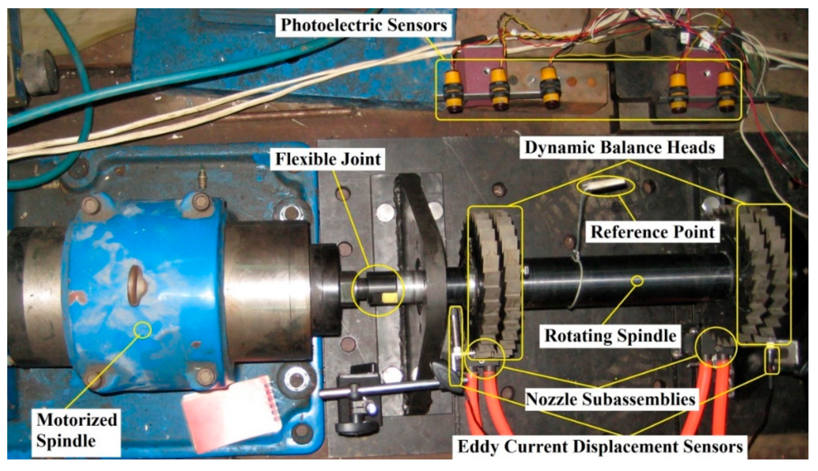
2. The Online Dynamic Balance System Design for Double-Face Correction

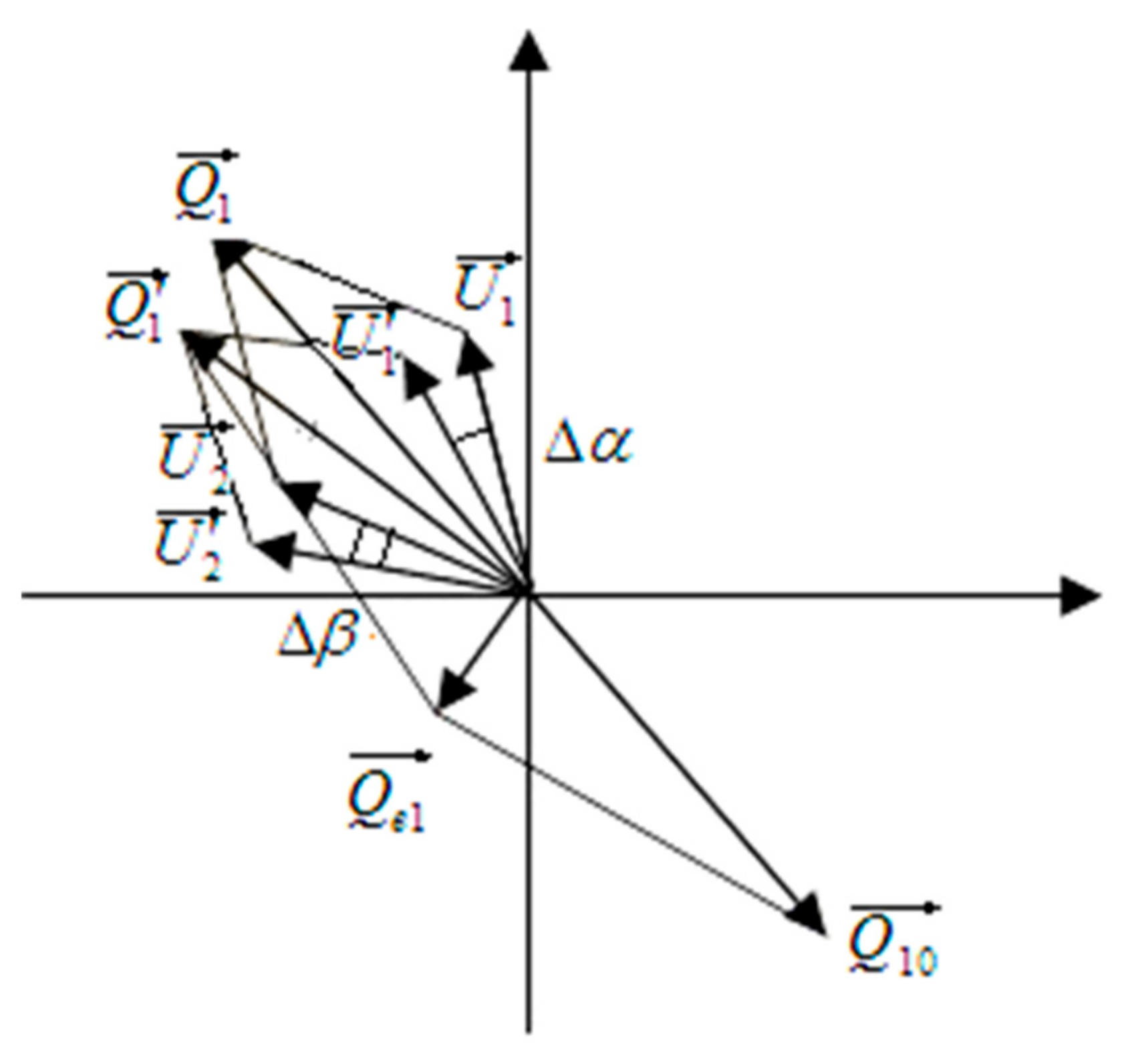
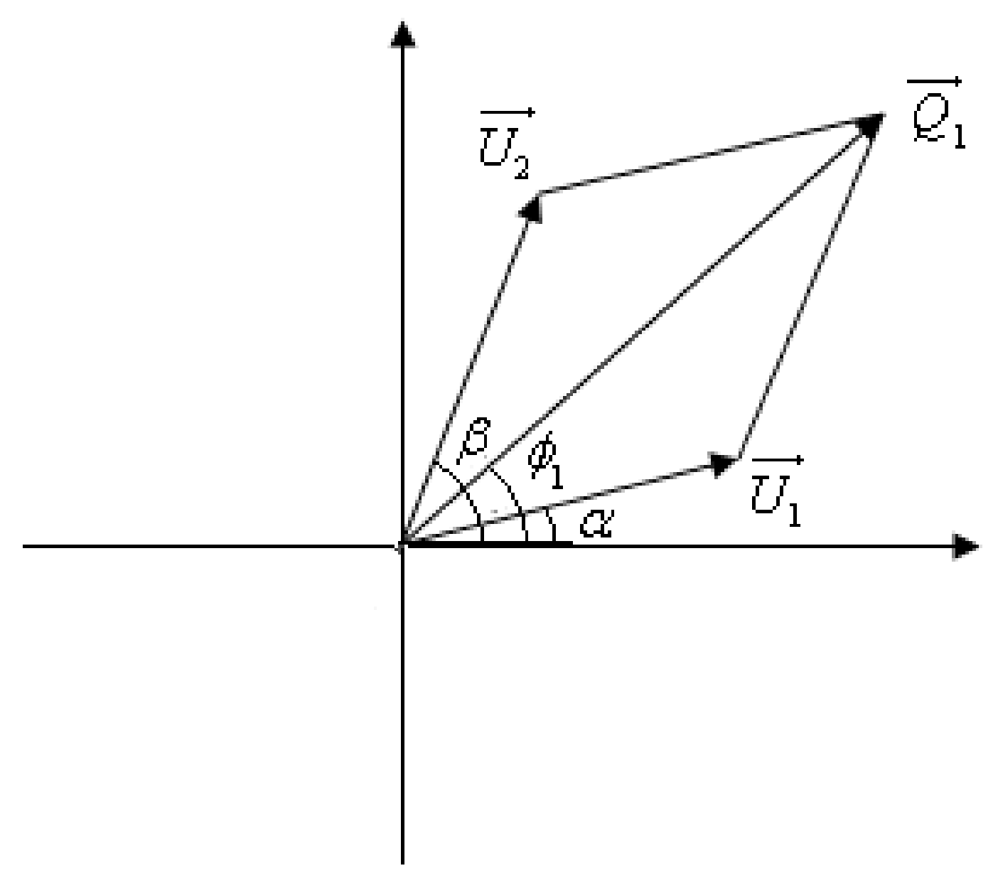
2.1. The Principle of Vector Synthesis

There are many methods to exert a suitable correcting vector in a correcting face. According to the vector synthesis principle, the correcting vector in one face can be synthesized by the two nearest balance disks with suitable fixed unbalance. As an example, the synthetic principle of a correcting vector is explained as follows.
Considering the structure characteristics of a balance disk, the fixed unbalance vector can be taken as a mass ball with a certain radius, and the centrifugal force comes into being when the mass ball rotates synchronously with the spindle. Because the axial positions of balance disks 1 and 2 are very close, their centrifugal force can be taken as in a face. The display of the vectors is shown in Figure 1.
In Figure 1, U 1 = U 1 α is assumed to be the fixed unbalance vector of balance disk 1, U1 and α represent the amplitude and phase of the vector separately. U 2 = U 2 β is assumed as the fixed unbalance vector of balance disk 2, U2 and β represent the amplitude and phase of the vector separately. In practical application, U 1 and U 2 can be taken as the correcting vector of balance disks 1 and 2 in theory. Q 1 = Q 1 ϕ 1 is assumed to be the correcting vector in face 1, Q1 and ϕ1 represent the amplitude and phase of the vector separately.
Based on the vector geometrical relationship in Figure 1, Equation (1) can be obtained.
{ U 2 sin ( φ 1 α ) = U 1 sin ( β φ 1 ) Q 1 2 = U 1 2 + U 2 2 2 U 1 U 2 cos ( 180 ° + α β )
In Equation (1), the parameters U1, U2, Q1, and ϕ1 are known, and the amplitudes of the unbalance vectors are designed to be equal (U1 = U2 = U) in practice, so the radial positions of the balance disks 1 (α) and 2 (β) can be calculated and expressed as follows.
{ β = ϕ 1 + 1 2 arccos Q 1 2 U α = ϕ 1 1 2 arccos Q 1 2 U
According to the above analysis, the synthetic correction in one face can be synthesized and obtained easily by adjusting the radial positions of the two balance disks. Proper corrections of the two correcting faces can be synthesized by four balance disks.

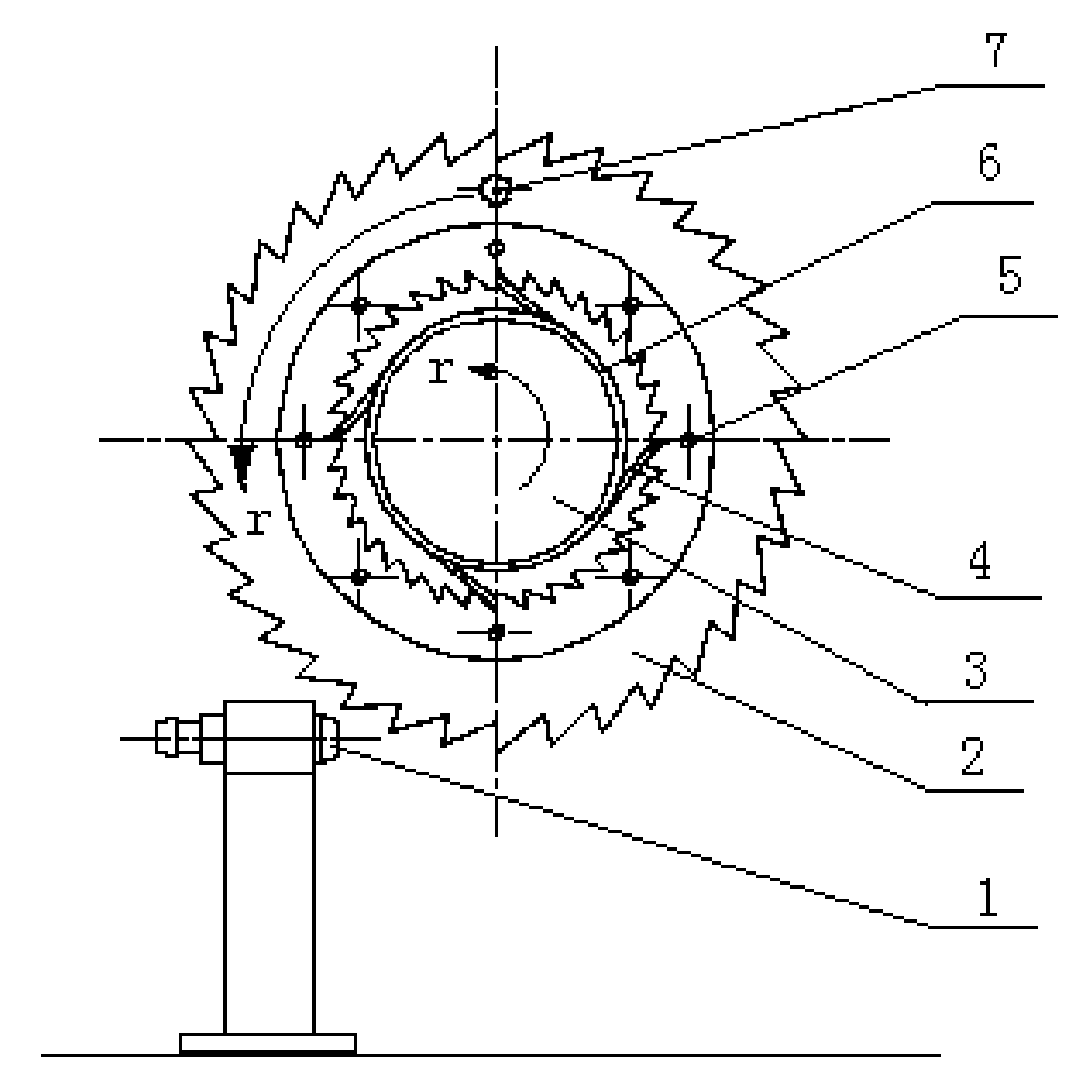
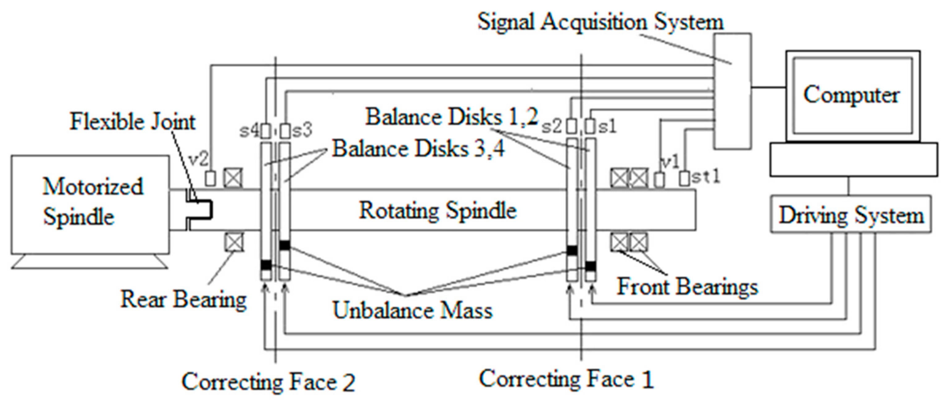
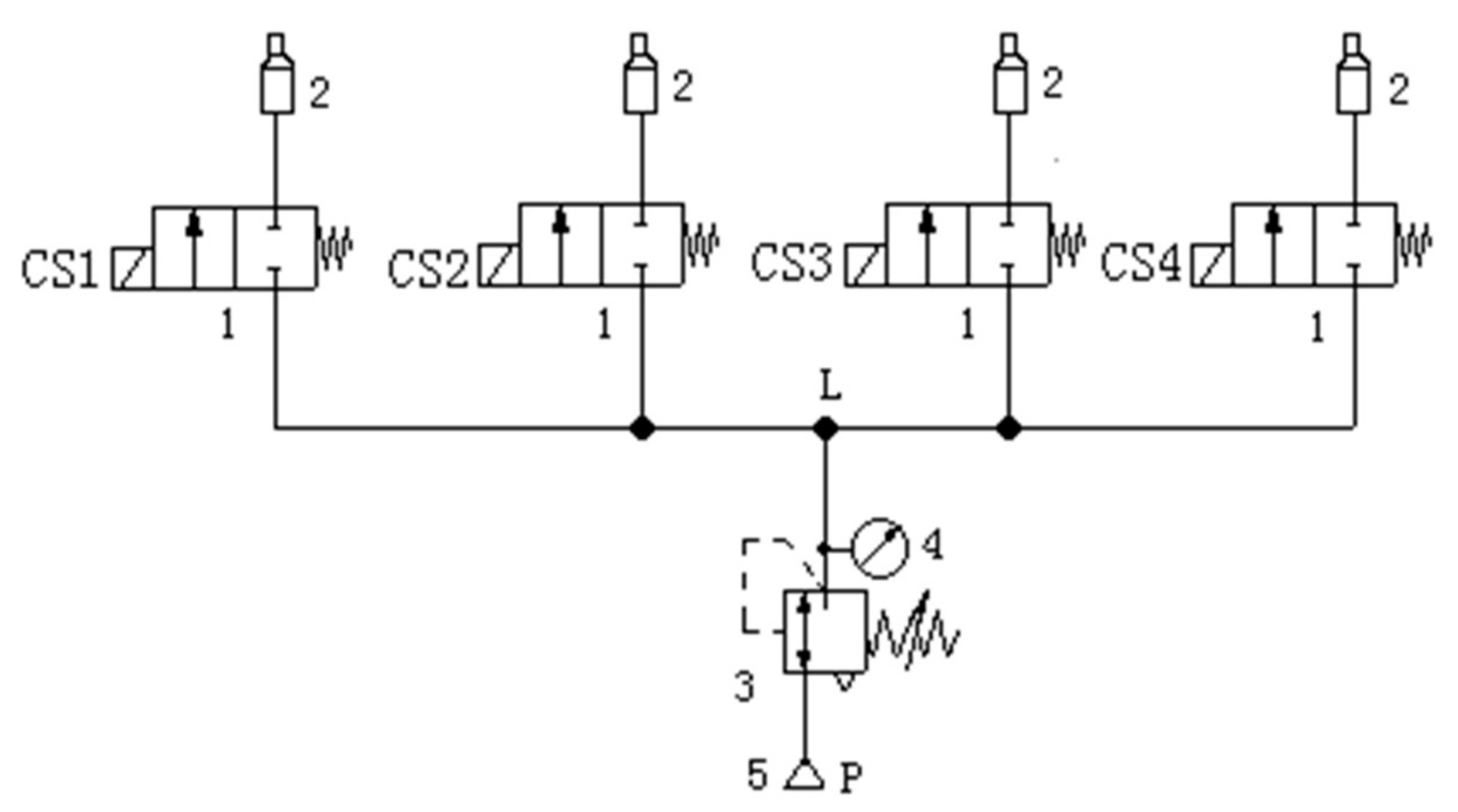
2.2. The Design of the Dynamic Balance Device and Driving System

Based on the principle of vector synthesis, four balance disks with equivalent fixed unbalance vector were applied to design the double-face correcting system for spindle dynamic balance and the experimental equipment was built. The measurement and control system is shown in Figure 2.
In Figure 2, the correcting vector ( Q 1 ) of face 1 can be synthesized by the balance disks 1 and 2, and the correcting vector ( Q 2 ) of face 2 can be synthesized by the balance disks 3 and 4. There is a flexible joint between the experimental device and motorized spindle. During the experiment, the vibration signals of the rotating spindle ends can be acquired by eddy current sensors v1 and v2, the radial positions signal of balance disks 1 to 4 can be acquired separately by the photoelectric sensors s1 to s4, and the radial positions signal on the spindle can be acquired by the photoelectric sensor st1. All the sensors’ signals can be collected by a signal acquisition system and analyzed online in the computer. The signal analysis process can be expressed as following.
First, the unbalance vibration signals are separated from the vibration signals of the spindle.
Second, when the amplitudes of the unbalance vibration signals exceed the allowable value, the correcting vectors in faces 1 and 2 are calculated according to the control law.
Third, the expected radial positions of balance disks 1 to 4 are calculated according to the required correcting vectors.
Fourth, the control signals are outputted from the computer and then the radial positions of balance disks 1 to 4 are adjusted to reach their expected position.
In order to meet the requirement of online control, a new type of balance disk structure and its driving system were developed as Figure 3 shows.
In Figure 3, the inside and outside circles are designed to be a dentate structure of the balance disk body. The installing ring with four elastic claws is installed between the spindle and balance disk body, and it is interference fit between the spindle and installing ring. Four nozzle mechanisms are installed separately under the corresponding balance disks. The working principle of the mechanism is illustrated as follows.
When the spindle system works in the balance condition, the installing ring is driven by the spindle to rotate synchronously, meanwhile the balance disk body is driven to rotate synchronously by a ratchet–pawl mechanism. On the contrary, a series of pulse air flows with high pressure are jetted from the nozzles to adjust the radial positions of the balance disk body. In theory, the phase corresponding to one tooth can be adjusted by one pulse air flow if the pressure and width of the pulse air flow are controlled properly.
To meet the requirement of online control, the pneumatic driving system is shown in Figure 4.
As Figure 4 shows, the driving pressure of pulse air flows can be controlled by adjusting the openness of the pressure regulating valve (3). The air pulse signal can be gained by controlling the magnetic valve to be on or off.

2.3. Discussion on the Balance Accuracy Problem of the Balance Disk Mechanism

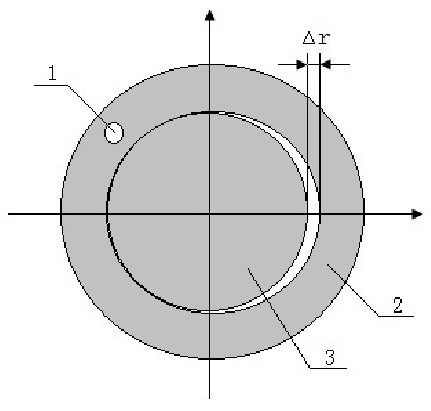
2.3.1. The Position Error Problem

According to the working principle in Figure 3, the tooth number of the balance disk is designed to be 72, the reachable positions of the balance disk include 0°, 5°, …, 355°. The nearest and reachable position will be considered as the expected position of the balance disk when the online calculated value is not equal to any reachable positions, so the maximum value of the position error is 2.5°. Because of the position error of the balance disk, the equivalent unbalance in a correcting face will not be offset by the composed correction. The residual unbalance is unavoidable and its derived principle is shown in Figure 5.
In Figure 5, Q 10 is the equivalent unbalance vector in face 1 from spindle system, U 1 and U 2 are the correcting vectors of balance disks 1 and 2 in theory, Q 1 is the synthetic correcting vector in theory. U 1 and U 2 are the correcting vectors of balance disks 1 and 2 in practice, Q 1 is the correcting vector in practice, Δα is the position error of balance disk 1, Δβ is the position error of balance disk 2, Q ε 1 is the residual unbalance. Based on the geometrical relationship in Figure 5, the residual unbalance can be expressed as Equation (3).
Q ε 1 = 2 Q 1 cos ( 90 ° Δ β Δ α 4 ) β α 2 3 ( Δ β Δ α ) 4 90 °
It can be seen from Equation (3), the amplitude of residual unbalance will be maximum when the sign of Δα and Δβ are opposite. For example, if Δα = Δβ = 2.5°,the maximum amplitude of residual unbalance is 0.0219 Q1, and this error is acceptable in most cases.

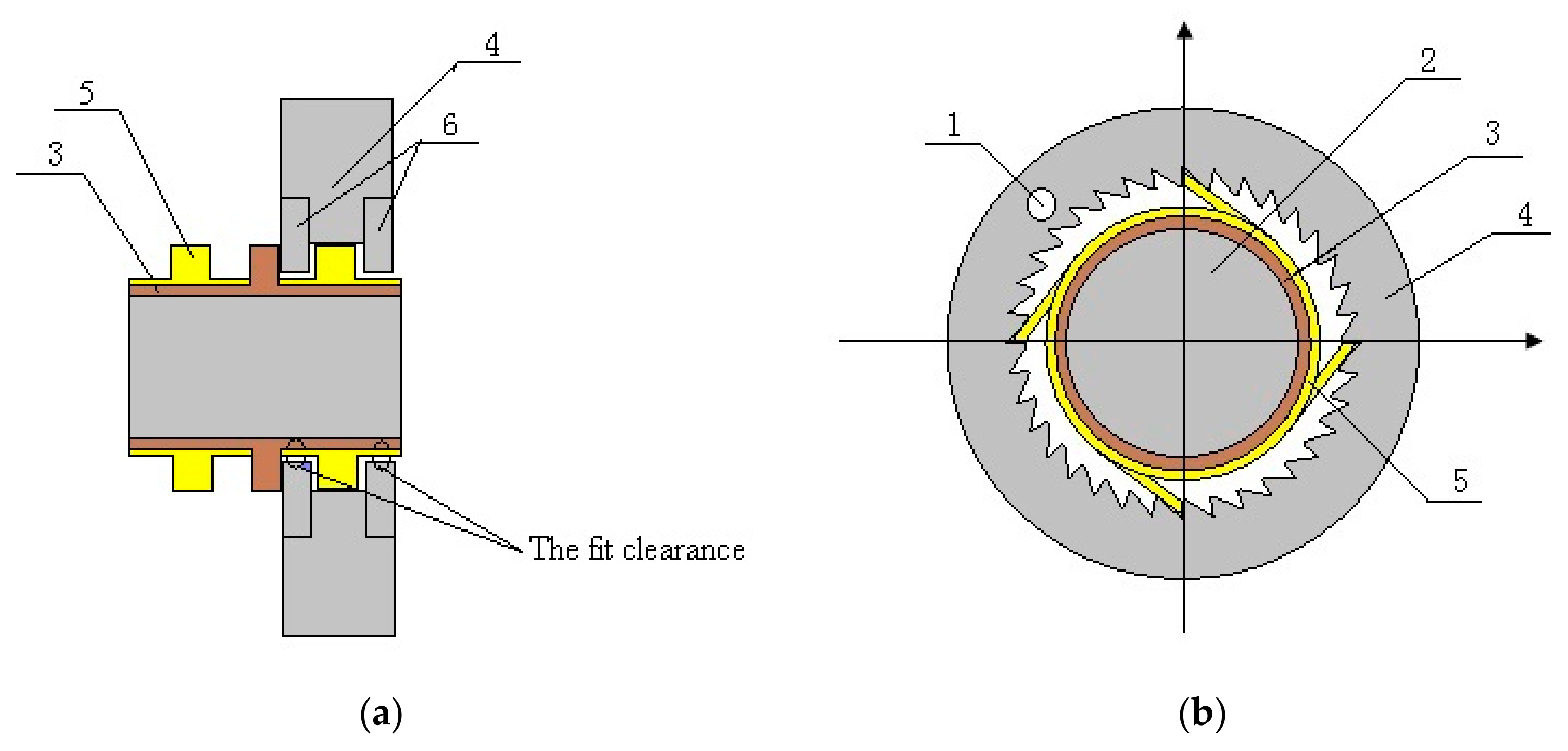
2.3.2. The Fit Clearance Problem

In order to ensure that the balance disk can be adjusted freely with respect to the spindle, a suitable clearance between the balance disk and spindle must be left. When the balance disk is driven to rotate synchronously with the spindle, the rotating center line of the balance disk will deviate from the center line of the spindle caused by centrifugal force, and the additional unbalance shown in Figure 6 will be formed as spindle rotary.
As Figure 6 shows, if the mass of balance disk is supposed as m, the additional unbalance can be expressed as Equation (4).
U a = m Δ r
In Equation (4), U a is the additional unbalance. Because the mass of the balance disk is large, the additional unbalance may be large even though the offset distance is small. In order to reduce the offset distance, the structure of the balance disk is improved to be a combined mechanism shown in Figure 7.
In Figure 7, the double-shoulder sleeve and installing ring are fixed on the spindle, the side covers are fixed in the balance disk, suitable fit clearance can be ensured by the double-shoulder sleeve and side covers. Figure 7b shows that the non-uniformity of the fit clearance is reduced by the outward elastic power of four elastic claws. So, the offset distance can be reduced between the balance disk and spindle.
Based on the above analysis, the main characteristics of the balance device proposed in the paper are summarized as follows compared with the related mechanisms.
(1)
The axial size of the balance device is small, and the synthetic vector of the two closer balance disks can be taken as in a face. In practical application, the structure of the machine tool spindle is very compact, and the balance device is difficult to apply in the actual machine tool if its axial size is larger.
(2)
According to the analysis in Section 2.3, the proposed balance device in the paper has symmetrical radial clearance between the balance disk and spindle whether it is in a stopping or running state, and the additional unbalance caused by the balance device is small.
(3)
The proposed balance device is a pure mechanical structure, and there is no electromagnetic interference in the motorized spindle system.
(4)
Location error may exist in the process of the radical position of the balance disk adjusted, but the maximum error can be accepted in application.

3. The Gain Parameter Adaption and Scheduling Control Method

The gain scheduling control method can be used to control the nonlinear system only if there are some control parameters under steady-state and a linear model that can reflect the system performance. Based on the online estimation method of the influence coefficient, we propose the gain parameter adaption and scheduling control method for spindle online dynamic balance. There are three main components of the method application, the gain table should be built first by many trial weight experiments. Then the gain parameters are indexed during the online dynamic balance period and the gain parameters are renewed when the system dynamic characteristics change.

3.1. The Double-Face Influence Coefficient Principle

In order to build the gain table, the double-face influence coefficient should be estimated by the trial weight method at a constant speed. The operating steps are stated as follows:
Step 1, the test speed, assumed as ω, must be selected, and then the initial unbalance vibration signal of testing points 1 and 2 is obtained by vibration signal measurment and analysis. The unbalance vibration vectors of points 1 and 2 are represented by V 01 and V 02 .
Step 2, the influence coefficients of correcting face 1 to points 1 and 2 can be calculated through trial weight experiments in correcting face 1. If the unbalance vibration vectors of points 1 and 2 are respectively assumed as V 11 and V 12 after trial weight in face 1, and the corresponding trial weight vector is P 1 , the influence coefficients can be represented as:
R 11 = V 11 V 01 P 1 ,   R 12 = V 12 V 02 P 1
In Equation (5), R 11 is the influence coefficient of correcting face 1 to point 1, R 12 is the influence coefficient of correcting face 1 to point 2.
Step 3, the influence coefficients of correcting face 2 to points 1 and 2 can be calculated through trial weight experiments in correcting face 2. If the unbalance vibration vectors of points 1 and 2 are respectively assumed as V 21 and V 22 after trial weight in face 2, and the corresponding trial weight vector is P 2 , the influence coefficients can be represented as:
R 21 = V 21 V 01 P 2 ,   R 22 = V 22 V 02 P 2
In Equation (5), R 21 is the influence coefficient of correcting face 2 to point 1, R 22 is the influence coefficient of correcting face 2 to point 2.
Combining Formulas (5) and (6), the double-face influence coefficient vector matrix (R) in the balance speed can be expressed as:
R = | R 11 R 21 R 12 R 22 |
Based on the above trial weight method, the work speed range of the spindle can be discretized to many balance speeds, the influence coefficient vector matrix of each balance speed can be tested and calculated. In order to improve the accuracy of the influence coefficient offline estimation, the method of averaging many times experimental values can be applied at each balance speed.

3.2. The Gain Scheduling Control Principle

When the influence coefficients of the balance speed have been estimated, a series of iteration controls are used to minimize the unbalance vibration amplitude, and the kth time iteration equation can be expressed as
V k = R P k + V 0
In Equation (8), Vk is the residual unbalance vibration matrix after the kth time iteration control. R is the influence coefficient matrix at the balance speed. Pk is the correcting matrix of the kth time correcting operation. V0 is the initial unbalance vibration matrix. The vector matrixes of Vk, R, Pk and V0 are expressed as follows
V k = [ V k 1 V k 2 ] T ,   R = | R 11 R 21 R 12 R 22 | ,   P k = [ P k 1 P k 2 ] T ,   V 0 = [ V 01 V 02 ] T
Based on Equation (8), the (k + 1)th time iteration equation can be expressed as:
V k + 1 = R P k + 1 + V 0
Vk+1 can be expressed by subtracting Equation (8) from Equation (9) as the following
V k + 1 = R [ P k + 1 P k ] + V k
According to the least square method, the generalized linear quadratic objective function can be built and shown as Equation (11).
J k + 1 = 1 2 V k + 1 T ¯ Q V k + 1 + 1 2 P k + 1 T ¯ H P k + 1
In Equation (11), H is a 2 × 2 positive definite real diagonal weighted matrix and is applied to improve the robustness and stability of the control system. Q is a 2 × 2 positive definite real diagonal weighted matrix and is applied to make the residual unbalance vibration of the testing points tend to equilibrium, so the diagonal values of Q should be set properly corresponding to the measuring points.
Equation (12) can be derived by substituting Equation (10) into Equation (11) and then simplifying the equation.
J k + 1 = 1 2 { R [ P k + 1 P k ] } T ¯ Q { R [ P k + 1 P k ] + V k ] } + 1 2 P k + 1 T ¯ H P k + 1
The function (13) can be derived by minimizing the objective function (12).
J k + 1 P k + 1 = R T ¯ Q { R [ P k + 1 P k ] + V k ] } + H P k + 1 = 0
Based on Equation (13), the following control law can be extracted.
{ P k + 1 = [ R T ¯ Q R + H ] 1 R T ¯ Q R P k [ R T ¯ Q R + H ] 1 R T ¯ Q V k = K 2 P k K 1 V k K 1 = [ R T ¯ Q R + H ] 1 R T ¯ Q , K 2 = K 1 R
In Equation (14), K1 and K2 are named as gain matrixes, which can be calculated when the influence coefficient matrix has been obtained. The gain scheduling table can be built and applied in the balance control when all the gain values have been calculated corresponding to each balance speed. In practical application, the work speed of the spindle may be not be equal to any balance speed with gain prameters, but the corresponding gain matrixes can be calculated by the linear interpolation method. If the work speed is assumed as ω, the two nearist balance speeds are assumed as ωj and ωj−1. The gain matrixes corresponding to ω can be calculated as follows.
{ K 1 ( ω ) = ω j ω ω j ω j 1 K 1 ( ω j 1 ) + ω ω j 1 ω j ω j 1 K 1 ( ω j ) K 2 ( ω ) = ω j ω ω j ω j 1 K 2 ( ω j 1 ) + ω ω j 1 ω j ω j 1 K 2 ( ω j )
Equation (14) indicates that the accuracy of the influence coefficient has a significant influence on the performance and stability of the dynamic balance control system. However, the influence coefficient error between the estimation value and the real value is inevitable on account of the balance system errors and working condition transformation. Here we discuss the effect of the influence coefficient error on the stability of the control system.
Assuming that the acceleration of the spindle is very small, the damping factor is very large and the discrete speed point is very dense in a certain range, we can take the dynamic characteristics of the system as close to steady state at various discrete speeds. If the system is stable at all discrete speeds, it can be assumed that the system is stable during the entire transmission period. When the speed is constant, Equation (10) is substituted to Equation (14) to obtain the following formula:
P k + 1 = K 2 P k K 1 R P k K 1 V k = [ K 2 K 1 R ] P k K 1 V k
P k + 1 = [ R ^ ¯ Q R ^ + H ] 1 R ^ ¯ Q [ R ^ R ] P k [ R ^ ¯ Q R ^ + H ] 1 R ^ ¯ Q V k
In Equation (17), R ^ is the estimated value of R, and R ^ - R is the error matrix of the influence coefficient. For stability control, the input of Pk+1 must converge to a constant vector. At the balance speed, the original unbalance vibration Vk of the rotor system is a constant vector. Because the estimated influence coefficient matrix is a constant matrix, the second item on the right of Equation (17) is the constant vector. Therefore the first item on the right of Equation (17) is related to stability. That is to say the condition for system stability is:
γ = δ max [ R ^ ¯ Q R ^ + H ] 1 R ^ ¯ Q [ R ^ R ] < 1
In Equation (18), γ represents the stability of the control system, δmax represents the maximum singular value of the matrix. Equation (18) can be translated as follows.
γ = δ max [ R ^ ¯ Q R ^ + H ] 1 R ^ ¯ Q [ R ^ R ] δ max R ^ ¯ Q δ max [ R ^ R ] δ min [ R ^ ¯ Q R ^ + H ] δ max R ^ ¯ Q δ max [ R ^ R ] δ min [ R ^ ¯ Q R ^ ] = ς
In Equation (19), δmin represents the minimum singular value of the matrix. ζ represents the stability of the traditional weighted least square method (WLSM) when H = 0, where the robustness of WLSM had been proved in paper reference [16]. It is obvious that the stability of the system can be increased by the unbalance correction penalty factor H.

3.3. The Adaptive Principle of the Influence Coefficient and Gain

The above algorithm shows that the gain scheduling control method is suitable for the kinetic parameters transformation with the working conditions, and the real influence coefficients do not need to be known when the gain scheduling control method is applied in rotor online dynamic balance. On the other hand, the gain schelduling control method belongs to the open loop control and no feedback and compensation mechanism for inaccurate gain. The dynamic balance practice shows that the influence coefficient of the high speed spindle system will transform even at the same speed with its working environment, working time, signal testing, and analysis accuracy. The gain, calculated in the offline state, cannot absolutely meet the requirement of online dynamic balance control. To improve the precision of online dynamic balance, the method of gain self-adaption is put forward in this paper based on the influence coefficient online estimation.

3.3.1. The Self-Adaption Methods of the Influence Coefficient

Based on the preceding text analysis, the kth time testing and calculating value (Rk) of the influence coefficient at the same balance speed can be expressed as.
R k = [ V k V k 1 ] [ P k P k 1 ] 1
The kth time estimated value ( R ^ k ) of influence coefficient can be obtained by the weighting average between the kth time testing and calculating value and the (k − 1)th time estimated value ( R ^ k 1 ).
R ^ k = A R k B + C R ^ k 1 D
In Equation (21), A, B, C, and D are a 2 × 2 diagonal matrix and named as forgetting factors. The diagonal values of A, B, C, and D belong to (0,1). The parameters in Equation (21) are assumed as follows.
A = | a 11 0 0 a 22 | , B = | b 11 0 0 b 22 | ,   C = | c 11 0 0 c 22 | , D = | d 11 0 0 d 22 | ,   R k = | R k 11 R k 12 R k 21 R k 22 |
Based on the above hypotheses, the influence coefficient of correcting face i relative to testing point j after kth time estimated can be expressed as follows.
R ^ k i j = a i i b j j R k i j + c i i d j j R ^ ( k 1 ) i j
The real influence coefficients at the same balance speeds are assumed as constant, the kth time testing and calculating value of influence coefficient can be expressed as Equation (23) in consideration of the random error.
R k i j = R i j + e
In Equation (23), Rij is the real influence coefficient, e is the uniform white noise signal. The transfer function of Equation (22) can be expressed as Equation (24) if Rkij is taken as the input signal and R ^ k i j is taken as the output signal.
G ( Z ) = a i i b j j 1 c i i d j j z 1
To ensure the signal is undistorted, G(1) = 1 when ω = 0. So, the relation among the forgetting factors can be obtained from Equation (24).
a i i b j j = 1 c i i d j j μ i j = a i i b j j
The variance ratio before and after the signal filtered can be obtained from Equations (24) and (25).
δ 1 2 δ 2 2 = 2 μ i j μ i j
Equation (26) indicates that the filtering effect will be better when μij tends to zero. A small value is suitable for μij if the kinetic parameters of the spindle system change slowly, and a large value is suitable for μij on the contrary. Based on the expected variance ratio, the value of μij can be calculated, and then the coefficient of A, B, C, and D can be calculated. The adaptive relation equation of the influence coefficient as Equation (22) can be set up between the current testing and caculating value and the original estimated value.

3.3.2. The Self-Adaption Methods of the Gain Parameters

Based on the above analysis, the gain parameters self-adaption and its application steps can be expressed as follows.
Step 1, the gain scheduling table should be built through a series of offline experiments at a few discrete speeds. The influence coefficients and gain parameters should be included corressponding to each discrete speed in the table.
Step 2, the unbalancing vibration signals of the spindle system should be measured and separated online in the monitoring period. The correcting vectors of the correcting faces should be calculated according to Equation (14) if the amplitude of the unbalancing vibration signals exceeds the limited value.
Step 3, the radial positions of the balance disks are adjusted online according to the correcting vectors based on the principle of vector synthesis. The unbalancing vibration signals of the spindle system are measured and separated online again, and then the amplitudes of the unbalancing vibration signals are reassessed. The new influence coefficients and gain paremeters are estimated online, and then the old parameters corresponding to the current balance speed are replaced by the new parameters. The estimated methods of the new parameters are expressed as follows.
The current influence coefficients corresponding to the balance speed in the scheduling table are taken as the original estimated value of R ^ ( k 1 ) , the current testing and caculating values of Rk are obtained according to Equation (20). The new estimated values of R ^ k can be calculated according to Equation (22), and then the gain parameters can be calculated and renewed by replacing the parameter of R by R ^ k in Equation (14).
Step 4, the step 2 and step 3 are carried out repeatedly until the amplitude of the unbalancing vibration signals is reduced to the allowed range.

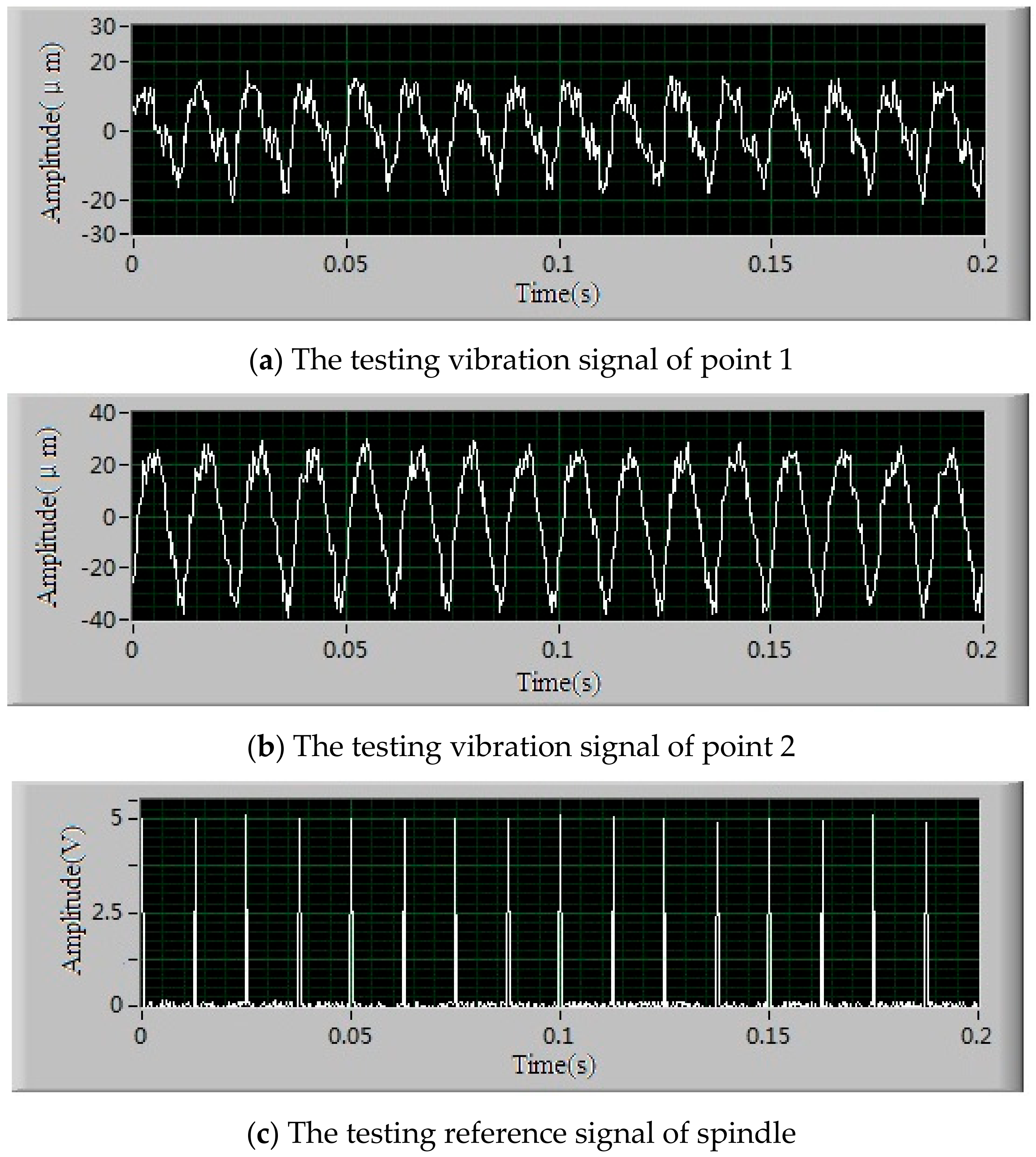
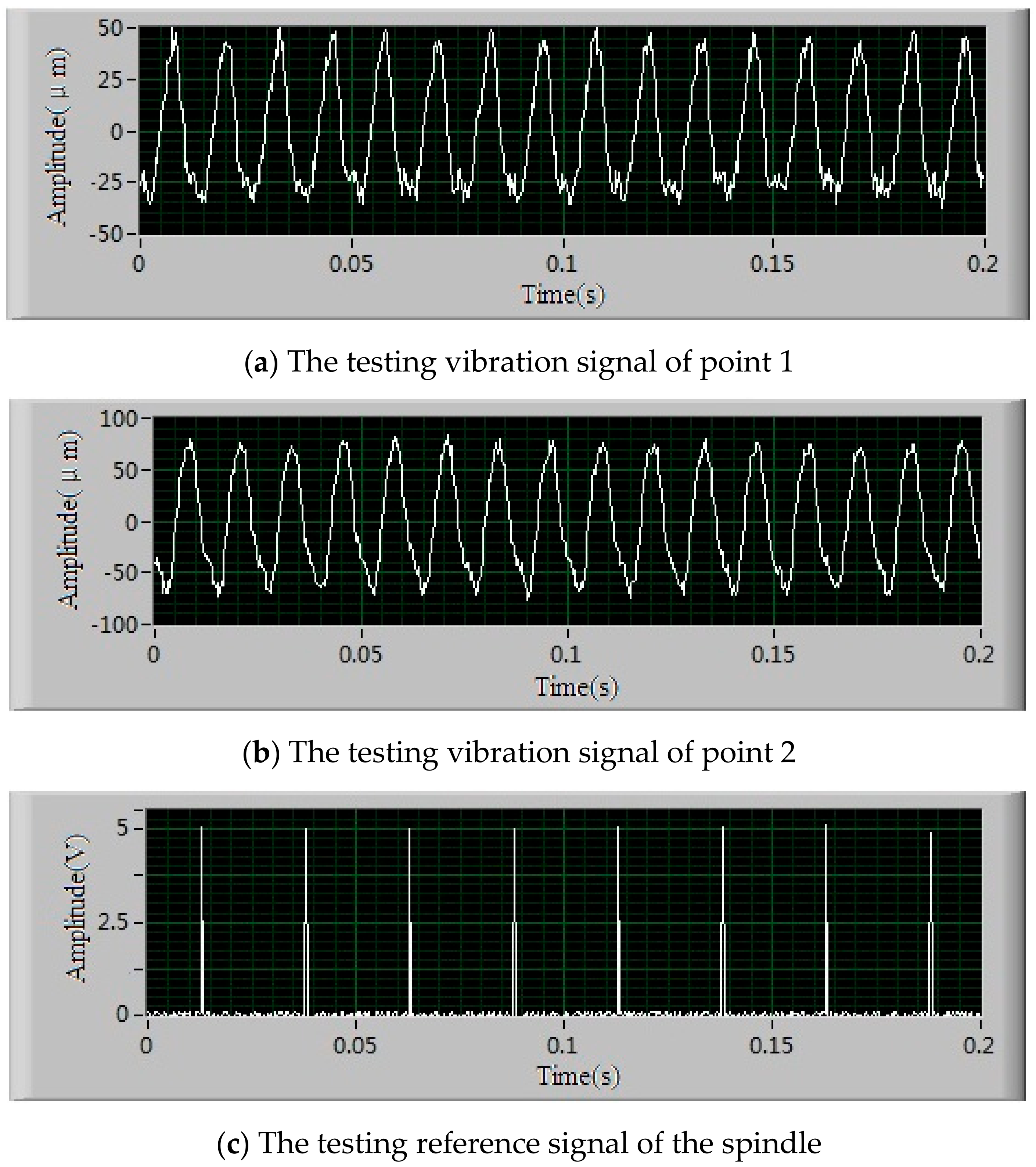
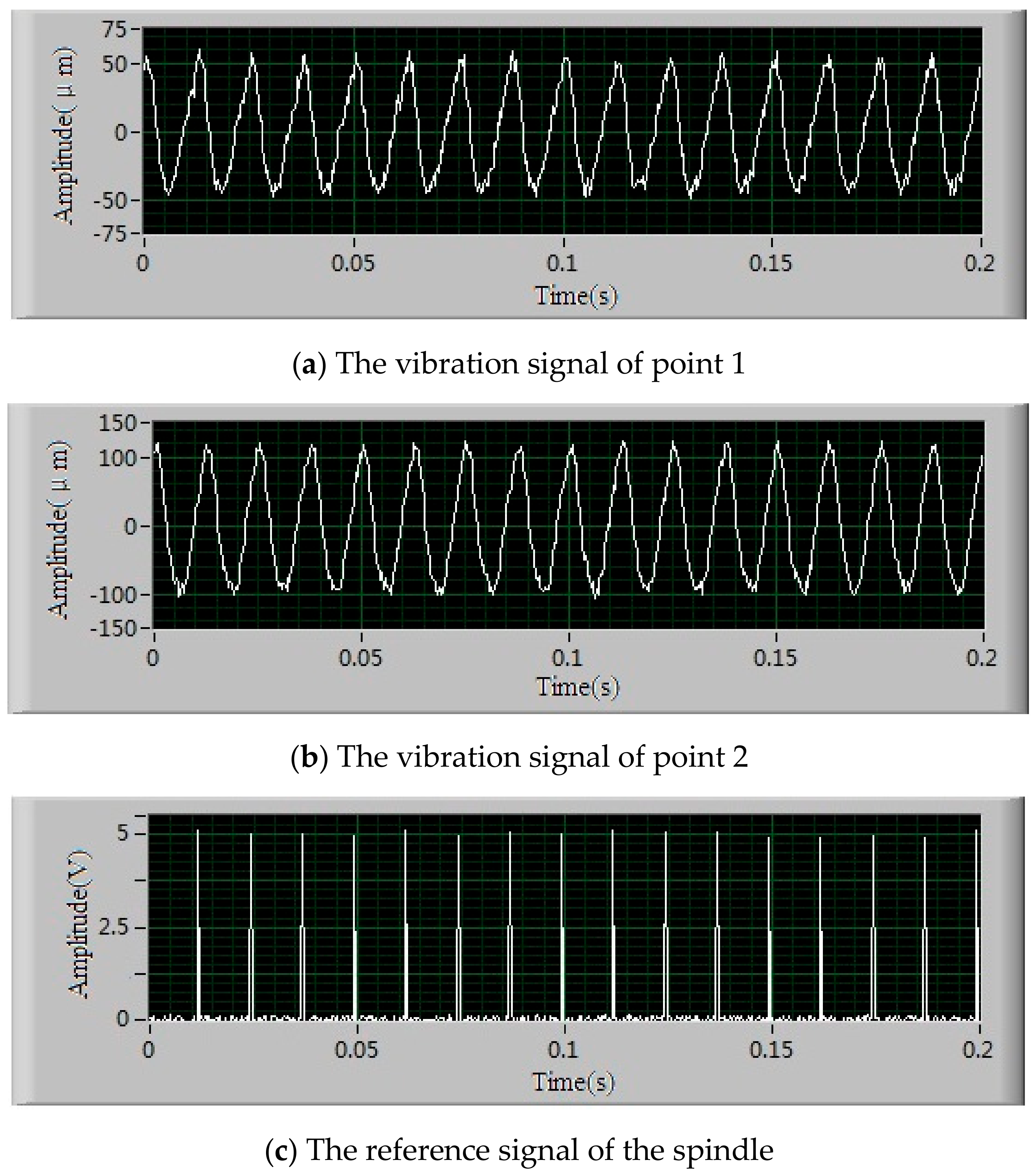
4. The Dynamic Balance Experiment and Its Result Analysis

The picture of the experimental system is shown as Figure 8. The motorized spindle is used to drive the rotating spindle with the dynamic balance mechanism to rotate synchronously. The sensors and signal acquisition system are used to collect the vibration signals, reference signal, and position signals. The pneumatic control system is used to drive the balance disks to reach the expected position. The software system is programmed by Labview language for signal acquisition, signal analysis, and output control.
According to the principle and steps of influence coefficient method, the influence coefficient change condition is examined by a series of trial weight experiments.
Step 1, Taken the balance speed of 4800 rpm as an example, the original vibration signals and reference signal are shown in Figure 9.
Comparing with the reference signal, the unbalance vibration vectors of points 1 and 2 are separated from the testing vibration signals by the least square method [17]. The separating results of unbalance vibration vectors are listed as follows.
V 01 = 11.35 μ m 3.3 ° ,   V 02 = 26.74 μ m 47.4 °
Step 2, The unbalance vector P 1 = 400 g cm 0 ° is exerted in correcting face 1, the spindle is run to the balance speed again, the testing signals of spindle are shown in Figure 10.
The unbalance vibration signals separated from the signals in Figure 10 are listed as follows.
V 11 = 36.32 μ m 117.2 ° ,   V 12 = 69.66 μ m 135.1 °
The influence coefficient of correcting face 1 relative to points 1 and 2 can be calculated as follows.
R 11 = 0.106 μ m / ( g cm ) 131.4 ° ,   R 12 = 0.185 μ m / ( g cm ) 156.3 °
Step 3, The unbalance vector P 2 = 560 g cm 90 ° is exerted in correcting face 2, the spindle is run to the balance speed again, and the testing signals of the spindle are shown in Figure 11.
The unbalance vibration signals separated from Figure 11 are listed as follows.
V 21 = 45.4 μ m 61.6 ° , V 22 = 103.5 μ m 52.1 °
The influence coefficient of correcting face 2 relative to points 1 and 2 can be calculated as follows.
R 21 = 0.075 μ m / ( g cm ) 40.8 ° ,   R 22 = 0.197 μ m / ( g cm ) 50.6 °
According to the above steps, the trial weight experiments are carried out once a month and the five times repeated experiment results are listed in Table 1.
In Table 1, the correcting vectors are calculated according to the current influence coefficient, the residual unbalance vibration vectors are tested after correcting vectors are exerted. It can be seen from Table 1, affected by the factors of kinetic parameter variation of the spindle system, adjustment error, measurement, and signal analysis error etc, that the differences of these influence coefficients are obvious even at the same speed. The correcting vectors and residual unbalance vibration vectors are affected directly by the influence coefficient.
Based on the data in Table 1, the adaptive process of influence coefficient and the gain parameters are shown in Table 2. For ease of calculation, the influence coefficient and gain parameters are expressed as the plural.
In Table 2, the forgetting factors are set to be 0.5I2×2, the weighting matrix H is set to be 8I2×2, and weighting matrix Q set to be 80I2×2. Based on the data in Table 2, the correcting vectors are calculated and the residual unbalance vibration are listed in Table 3.
In Table 3, the correcting vectors C R are calculated according to the adaptive influence coefficient, the correcting vectors C G are calculated according to the gain parameters. It can be seen from Table 3, the influence coefficient accuracy and the balance accuracy have been improved through the adaptive method. Compared with the balance effect of the influence coefficient method, the correcting vectors tend to be stable and close to the ideal value based on the adaptive gain scheduling control. Meanwhile, the residual unbalance vibrations of the testing points tend to be average and small. The more that the balance time is at the same speed, the more accurate the gain value and the much better the balance effect are.
In order to demonstrate the effectiveness of the proposed method in this paper, the other experimental results are shown as Table 4 based on the same method above.
It can be seen from Table 4, that a good balance effect has been obtained at other balance speeds, and the gain parameters adaption and scheduling control method proposed in this paper is effective.

5. Conclusions

(1)
The influence coefficient method is the common method for rotor online dynamic balance. The experiments proved that the precision of influence coefficient can be affected by transformation of speed, service time, environment condition, temperature field, abrasion, and lubrication condition of the supporting components, signal measurement and calculation accuracy etc. The accuracy of the influence coefficient has a big effect on the accuracy of online dynamic balance.
(2)
The accuracy of the influence coefficient can be improved by the self-adaptive method proposed in this paper. The experiments have proved that the balance accuracy can be improved and the trial weight times can be reduced.
(3)
In theory, we do not need to know the real influence coefficient when the gain scheduling method is applied in online dynamic balance, but the gain schelduling control method belongs to the open loop control and no feedback and compensation mechanism for the inaccurate gain. Based on the self-adaptive method of the influence coefficient, a self-adaptive method for gain parameters is proposed in the paper. The experiments prove that the balance accuracy can be improved based on the gain parameters self-adaptive method, and the residual unbalance vibration differences between the testing points can be reduced by adjusting the parameters of the weighting matrix.

Author Contributions

Conceptualization, S.Z. and Y. W.; Methodology, S.Z. and Z.Z.; Software, S.Z.; Validation, S.Z., Y.W. and Z.Z.; Formal Analysis, Y.W. and Z.Z.; Investigation, S.Z. and Z.Z.; Resources, S.Z., Y.W. and Z.Z.; Data Curation, S.Z. and Z.Z.; Writing-Original Draft Preparation, S.Z.; Writing-Review & Editing, S.Z., Y.W. and Z.Z.; Visualization, S.Z; Supervision, S.Z.; Project Administration, S.Z., Y.W. and Z.Z.; Funding Acquisition, S.Z. and Z.Z.

Acknowledgments

This work was supported by the National Natural Science Foundation of China (No. 51605332), the science and technology funds from Tianjin Municipal Education Commission (No. 2017KJ110).

Conflicts of Interest

The authors declare no conflict of interest.

References

  1. Jung, D.Y.; DeSmidt, H. A new hybrid observer based rotor imbalance vibration control via passive auto-balancer and active bearing actuation. J. Sound Vib. 2018, 415, 1–24. [Google Scholar] [CrossRef]
  2. Xiang, M.; Wei, T. Auto-balancing of high-speed rotors suspended by magnetic bearings using LMS adaptive feed-forward compensation. J. Vib. Control 2014, 20, 1428–1436. [Google Scholar] [CrossRef]
  3. Zheng, S.Q.; Han, B.C.; Feng, R.; Jiang, Y.X. Vibration Suppression Control for AMB-Supported Motor Driveline System Using Synchronous Rotating Frame Transformation. IEEE Trans. Ind. Electron. 2015, 62, 5700–5708. [Google Scholar] [CrossRef]
  4. Choi, W.H.; Yang, B.S.; Joo, H.J. Optimum field balancing of ratating machinery using genetic algorithm. Trans. Korean Soc. Mech. 1996, 20, 1819–1826. [Google Scholar]
  5. Hu, B.; Fang, Z.C. Gain-scheduling control of steady-state active balancing system of speed-varying rotor. Chin. J. Appl. Mech. 2006, 23, 137–141. [Google Scholar]
  6. Koo, J.H.; Kim, I.H.; Hur, N.S. A study on balancing of high speed spindle using influence coefficient method. J. Korean Soc. Manuf. Process Eng. 2012, 11, 104–110. [Google Scholar]
  7. Bin, G.F.; Li, X.J.; Shen, Y.P.; Wang, W.M. Development of whole-machine high speed balance approach for turbomachinery shaft system with N+1 supports. Measurement 2018, 122, 368–379. [Google Scholar] [CrossRef]
  8. Carbajal, F.B.; Navarro, G.S.; Montiel, M.A. Active unbalance control of rotor systems using on-line algebraic identification methods. Asian J. Control 2013, 15, 1627–1637. [Google Scholar] [CrossRef]
  9. Kim, J.S.; Lee, S.H. The stability of active balancing control using influence coefficients for a variable rotor system. Int. J. Adv. Manuf. Technol. 2003, 22, 562–567. [Google Scholar] [CrossRef]
  10. Moon, J.D.; Kim, B.S.; Lee, S.H. Development of the active balancing device for high-speed spindle system using influence coefficients. Int. J. Mach. Tools Manuf. 2006, 46, 978–987. [Google Scholar] [CrossRef]
  11. Hannoun, H.; Hilairet, M.; Marchand, C. High performance current control of a switched reluctance machine based on a gain-scheduling PI controller. Control Eng. Pract. 2011, 19, 1377–1386. [Google Scholar] [CrossRef]
  12. Wang, S.J.; Liao, M.F. A method for online control of sudden unbalanced vibration response of rotor. Mech. Sci. Technol. Aerosp. Eng. 2012, 233, 77–80. [Google Scholar]
  13. Fang, J.; Xu, X.; Xie, J. Active vibration control of rotor imbalance in active magnetic bearing systems. J. Vib. Control 2013, 21, 684–700. [Google Scholar] [CrossRef]
  14. Xu, J.; Zhao, Y.; Jia, Z.; Zhang, J. Rotor dynamic balancing control method based on fuzzy auto-tuning single neuron PID. IEICE Electron. Express 2017, 14, 20170130. [Google Scholar] [CrossRef]
  15. Zhang, L.; Luo, L.; Xu, J. An improved adaptive control method for active balancing control of rotor with time-delay. IEICE Electron. Express 2017, 14, 20171069. [Google Scholar] [CrossRef]
  16. Knospe, C.R.; Hope, R.W.; Tamer, W.M. Robustness of adaptive unbalance control of rotors with magnetic bearings. J. Vib. Control 1996, 2, 33–52. [Google Scholar] [CrossRef]
  17. Zhang, S.H.; Cai, Y.J. A new double-face online dynamic balance device and its control system for high speed machine tool spindle. J. Vib. Control 2016, 22, 1037–1048. [Google Scholar]
Figure 1. The synthetic principle of the correcting vector in a face.
Applsci 08 00917 g001
Figure 2. The double-face online dynamic balance system.
Applsci 08 00917 g002
Figure 3. The structure principle of the balance disk. Notes: 1 Nozzle mechanism; 2 balance disk body; 3 spindle; 4 elastic claw; 5 thread hole; 6 installing ring; 7 unbalance hole.
Applsci 08 00917 g003
Figure 4. The pneumatic control system. Notes: 1 two-position two-way valve; 2 nozzle; 3 pressure regulating valve; 4 pressure gage; 5 air source.
Applsci 08 00917 g004
Figure 5. The radial position error of the balance disk.
Applsci 08 00917 g005
Figure 6. The deriving principle of additional unbalance. Notes: 1 unbalance mass; 2 balance disk; 3 spindle; ∆r offset distance.
Applsci 08 00917 g006
Figure 7. The compensation principle of the fit clearance. (a) The fit condition between balance disk and spindle; (b) The four claws structure of balance disk. Notes: 1 unbalance mass; 2 spindle; 3 double-shoulder sleeve; 4 balance disk body; 5 installing ring; 6 side covers.
Applsci 08 00917 g007
Figure 8. Picture of the experimental system.
Applsci 08 00917 g008
Figure 9. The original vibration signals and reference signal of the spindle.
Applsci 08 00917 g009
Figure 10. The original vibration signals and reference signal of the spindle after the first trial weight.
Applsci 08 00917 g010
Figure 11. The original vibration signals and reference signal of the spindle after the second trial weight.
Applsci 08 00917 g011
Table 1. The results of trial weight and dynamic balance experiments of the influence coefficient method.
Testing TimesThe Influence Coefficient (μm/(g·cm)∠°)The Correcting Vector (g·cm∠°)Residual Unbalance Vibration Vector (μm∠°)
1 R 1 = [ 0.1055 131.4 0.1849 156.3 0.0748 40.8 0.1968 50.6 ] C = [ 145.1 14.8 124.1 122.3 ] V = [ 5.57 156.4 9.58 135 ]
2 R 2 = [ 0.1026 132.1 0.2025 165.5 0.0881 40.9 0.2292 51.9 ] C = [ 111.7 42.2 65.6 126.6 ] V = [ 5.84 146.5 8.79 122.1 ]
3 R 3 = [ 0.0922 134.5 0.1806 156.5 0.0788 40.9 0.2047 51.9 ] C = [ 110.5 41.9 66.2 127.6 ] V = [ 6.26 165.3 8.99 141.6 ]
4 R 4 = [ 0.0941 142.1 0.1996 165.6 0.0539 43.2 0.1598 45.1 ] C = [ 188.1 30.9 205 173.2 ] V = [ 7.13 166.3 11.25 124.8 ]
5 R 5 = [ 0.1148 142.1 0.2289 165.5 0.0987 52.1 0.2224 75.5 ] C = [ 145.4 30 127.4 176.1 ] V = [ 8.57 160 10.89 140.4 ]
Table 2. The self-adaptive process of influence coefficient and gain parameter.
TimesThe Self-Adaptive Influence Coefficient (μm/(g·cm))The Self-Adaptive Gain Parameter
K1K2
1 [ 0.0698 0.0791 i 0.1693 0.0743 i 0.0566 0.0489 i 0.1249 0.1521 i ] [ 0.6904 0.6629 i 0.4306 0.4952 i 1.3712 0.7399 i 1.1735 1.1757 i ] [ 0.0041 + 0.0518 i 0.0461 + 0.0362 i 0.0461 + 0.0362 i 0.145 0.0981 i ]
2 [ 0.0693 0.0776 i 0.1827 0.0625 i 0.0616 0.0533 i 0.1332 0.1662 i ] [ 0.6339 0.684 i 0.4918 0.4886 i 1.3674 0.7208 i 1.2831 1.1358 i ] [ 0.0049 + 0.0403 i 0.0573 + 0.0178 i 0.0573 + 0.0178 i 0.1868 0.1474 i ]
3 [ 0.067 0.0717 i 0.1742 0.0673 i 0.0606 0.0524 i 0.1297 0.1637 i ] [ 0.6086 0.645 i 0.5074 0.4711 i 1.3466 0.7664 i 1.2855 1.1777 i ] [ 0.0005 + 0.0317 i 0.0513 + 0.0091 i 0.0513 + 0.0091 i 0.157 0.1391 i ]
4 [ 0.0706 0.0648 i 0.1837 0.0585 i 0.0499 0.0447 i 0.1213 0.1384 i ] [ 0.6172 0.512 i 0.3471 0.4064 i 1.3781 0.5417 i 1.0208 0.9824 i ] [ 0.0096 + 0.0403 i 0.0693 + 0.0328 i 0.0693 + 0.0328 i 0.2093 0.0804 i ]
5 [ 0.0806 0.0676 i 0.2027 0.0579 i 0.0553 0.0613 i 0.0885 0.1769 i ] [ 0.7273 0.5484 i 0.424 0.5548 i 1.7084 0.5724 i 0.8357 1.4708 i ] [ 0.011 + 0.0367 i 0.055 + 0.0292 i 0.055 + 0.0292 i 0.1269 0.063 i ]
Table 3. The balance effect analysis.
Testing TimesThe Balance Effect of Influence Coefficient MethodThe Balance Effect of Gain Scheduling Method
The Correcting Vectors (g·cm∠°)The Residual Unbalance Vibration vector (μm∠° )The Correcting Vectors (g·cm∠°)The Residual Unbalance Vibration Vector (μm∠°)
1 C R = [ 145.1 14.8 124.1 122.3 ] V = [ 5.57 156.4 9.58 135 ] C G = [ 133.5 47.3 168.3 127.9 ] V = [ 5.21 25.7 9.05 54 ]
2 C R = [ 272.18 45 144.13 157 ] V = [ 6.22 29.6 9.51 121.5 ] C G = [ 204.5 43.2 157.9 145.7 ] V = [ 3.49 14 6.11 33 ]
3 C R = [ 209.89 36.9 178.51 147.2 ] V = [ 4.86 127.6 10.3 95.1 ] C G = [ 227.9 47.1 165.8 150.9 ] V = [ 4.79 45 5.91 63.4 ]
4 C R = [ 231.09 65.6 108.2 153.4 ] V = [ 6.93 89.6 9.2 5.7 ] C G = [ 237.33 48.7 168.85 153.1 ] V = [ 5.11 12.3 6.07 49.6 ]
5 C R = [ 240.1 60.3 128.2 162.5 ] V = [ 5.77 73.5 9.81 112.6 ] C G = [ 252.67 51.62 173.56 156.95 ] V = [ 4.17 48.1 5.18 33.7 ]
Table 4. The other experimental results.
Testing TimesThe Balance Speed: 5200 rpm
The Initial Unbalance Vibration:
V 01 = 16.42 μ m 10.3 °
V 02 = 32.32 μ m 37.2 °
The Balance Speed: 5600 rpm
The Initial Unbalance Vibration:
V 01 = 21.65 μ m 14.1 °
V 02 = 36.96 μ m 31.9 °
The Correcting Vectors (g·cm∠°)The Residual Unbalance Vibration Vector (μm∠°)The Correcting Vectors (g·cm∠°)The Residual Unbalance Vibration Vector (μm∠°)
1218.07∠−72.2
136.9∠144.8
6.82∠−69.9
8.41∠89.6
240.02∠−99.2
173.38∠121.1
8.46∠−99.9
9.66∠120.5
2227.74∠−71.2
140.26∠139.7
6.21∠−64.6
7.69∠75.3
236.66∠−76.4
171.91∠115.1
8.6∠−18.1
10.2∠108.1
3227.12∠−59.2
139.16∠135.8
5.9∠−70.7
6.56∠106.5
211.03∠−60.2
122.5∠144.9
8.27∠−31.2
9.62∠121.2
4228.91∠−58.9
139.65∠134.7
5.05∠−63.4
6.75∠175.8
222.48∠−65.3
123.3∠141.5
8.35∠−35
10.01∠126
5231.56∠−58.5
140.28∠132.8
5.87∠−53.2
6.26∠158.1
192.7∠−70.2
166.2∠145.8
8.59∠−39.8
9.88∠130.4

