Numerical Assessment of the Convective Heat Transfer in Rotating Detonation Combustors Using a Reduced-Order Model

Abstract

The pressure gain across a rotating detonation combustor offers an efficiency rise and potential architecture simplification of compact gas turbine engines. However, the combustor walls of the rotating detonation combustor are periodically swept by both detonation and oblique shock waves at several kilohertz, disrupting the boundary layer, resulting in a rather complex convective heat transfer between the fluid and the solid walls. A computationally fast procedure is presented to calculate this extraordinary convective heat flux along the detonation combustor. First, a numerical model combining a two-dimensional method of characteristics approach with a monodimensional reaction model is used to compute the combustor flow field. Then, an integral boundary layer routine is used to predict the main boundary layer parameters. Finally, an empirical correlation is adopted to predict the convective heat-transfer coefficient to obtain the bulk and local heat flux. The procedure has been applied to a combustor operating with premixed hydrogen–air fuel. The results of this approach compare well with high-fidelity unsteady Reynolds-averaged Navier–Stokes three-dimensional simulations, which included wall refinement in an unrolled combustor. The model demonstrates that total pressure has an important influence on heat flux within the combustor and is less dependent on the inlet total temperature. For an inlet total pressure of 0.5 MPa and an inlet total temperature of 300 K, a peak time-averaged heat flux of 6 MW/m² was identified at the location of the triple point, followed by a decrease downstream of the oblique shock, to about 4 MW/m². Maximum discrepancy between the reduced-order model and the high-fidelity solver was 16%, but the present reduced-order model required a computational time of only 200 s, that is, about 7000 times faster than the high-fidelity three-dimensional unsteady solver. Therefore, the present tool can be used to optimize the combustor cooling system.

1. Introduction

Rotating detonation combustors represent a potential efficiency leap for gas turbine power plants [1]. This boost in efficiency is due to the pressure gain obtained through the detonation process, which leads to a more efficient thermal cycle. A rotating detonation combustor is characterized by an annular channel where combustible mixture is injected and ignited by a self-sustained spinning detonation front at supersonic speeds. However, practical implementation is currently constrained by important thermal management issues due to the high-speed flow and high temperature levels reached inside the combustor. The combustor walls are periodically swept by shock waves at several kilohertz, which results in extraordinary heat-flux levels that limit the operability of the combustor. Therefore, it is critical to perform a detailed analysis of the convective heat transfer and develop predictive tools that allow a preliminary design of the cooling system. To address this issue, we present a reduced-order model that predicts the convective heat transfer in a rotating detonation combustor (RDC) with a numerical approach that is three orders of magnitude faster than three-dimensional unsteady Reynolds-averaged solvers.

RDCs have been experimentally tested, for example, in the US [2,3,4], Japan [5], Russia [6] and France [7]. The tests uncovered enormous heat-flux release threatening the integrity of the combustor and limiting its runtime to fractions of a second. The thermal optimization of these combustors is constrained by the availability of precise and time-effective thermal solvers that can evaluate the thermal performance in a timely manner. Currently, RDCs are numerically examined with computationally-expensive Euler [8,9] or unsteady Reynolds-averaged Navier–Stokes solvers [10], where the injection process is either modeled as premixed mixture or as non-premixed flow. The detonation process can be modeled in several ways: using one-step reaction kinetics [11] with a limited number of species; or with two-step chemical reaction models [12]; or with an induction parameter which allows for larger grid size and time steps [13,14,15,16]; or with detailed reaction kinetics [17] which lead to expensive computations. Due to the use of a coarse computational grid, most of the Navier–Stokes (URANS) simulations cannot resolve the boundary layer with sufficient accuracy to predict the actual convective heat-transfer level. Therefore, we need to develop time-efficient models that can provide a fast and accurate calculation of the heat-flux levels to allow a proper design of the necessary cooling strategies. Mizener and Lu [18] presented a low-order analytical performance model to determine the range of design parameters on the performance of rocket-mode RDCs. Fievisohn and Yu [19] presented a reduced-order model based on the two-dimensional method of characteristics (MOC) and the detonation conditions. Similarly, Sousa et al. [20] demonstrated via a reduced-order model based on a two-dimensional MOC that the system naturally evolves to a specific radius to detonation height ratio that minimizes entropy rise across the combustor.

Regarding heat-transfer analysis, Roy et al. [21] estimated the heat load within the RDC walls with unsteady conduction simulations using OpenFoam with periodic convective boundary conditions. Olcucuoglu et al. [22] developed a conjugate heat-transfer model within the same open-source flow solver. Theuerkauf et al. [23] measured the heat flux within the walls of a RDC using high-frequency heat-flux gages and observed an almost constant heat flux along the axial position. In 2018, Meyer et al. [24] measured the instantaneous and bulk heat fluxes for several equivalence ratios with a twelve-sensor heat-flux gage array.

This paper first evaluates the boundary layer in the RDC with URANS simulations. Afterwards, the URANS result is compared with the in-house developed two-dimensional model [20] that uses a semi-empirical correlation to predict the aero–thermal properties of the boundary layer. Furthermore, the paper identifies the locations of the heat-flux peaks, and corresponding streamwise evolution. This new reduced-order model can guide RDC research with estimates of the heat-transfer distribution necessary to design the cooling system, select the material, and determine the life of the model. Additionally, these results can be used to manage future experimental tests and select an adequate range of heat-flux sensors and their time/space resolution.

2. Aero–Thermal Modeling of Rotating Detonation Combustors

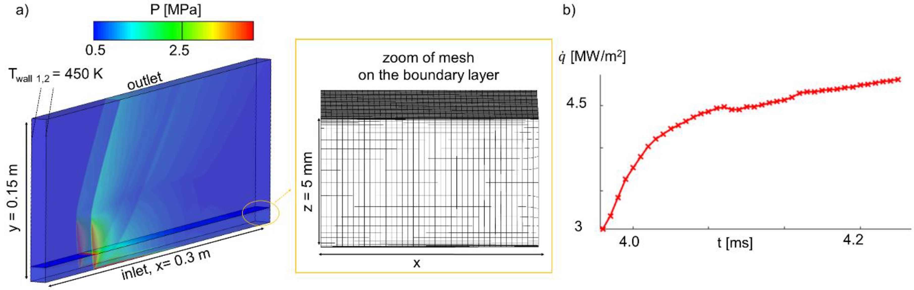
2.1. Unsteady Reynolds-Averaged Navier–Stokes Evaluation

The commercial software CFD++ developed by Metacomp Technologies [25] was used for the numerical simulations and was based on a finite-volume density-based solver. The convective fluxes were calculated with the Harten-Lax-Van Leer-contact approximate Riemann scheme. Interpolation of the spatial variables was performed through a second-order total variation diminishing (TVD) polynomial interpolation with a continuous limiter for stability reasons. We used an implicit time-integration method based on dual-time stepping with fixed global timestep and local Courant–Friedrichs–Lewy (CFL) number variation. Local iteration was accelerated through a multigrid acceleration scheme based on 4 multigrid cycles. The residual convergence criterion for each inner timestep was 0.1.

The governing Navier–Stokes equations are expressed as:

$$\frac{\partial \mathrm{Q}}{\partial \mathrm{t}}+\frac{\partial \left({\mathrm{F}}_1 +G_1\right)}{\partial \mathrm{x}}+\frac{\partial \left({\mathrm{F}}_2+G_2\right)}{\partial \mathrm{y}}+\frac{\partial \left({\mathrm{F}}_3+G_3\right)}{\partial \mathrm{z}}=\dot{S},$$

(1)

where $\mathit{Q}$ is representing the dependent variables, F the inviscid flux vectors, G the viscous flux vectors and $\dot{S}$ the source terms. Below, Equation (2) represents the inviscid, source and viscous flux vectors of Equation (1).

$$\mathit{Q}=\left(\begin{array}{c}e\\ \rho \\ \rho u\\ \rho v\\ \rho w\\ \rho {\sigma }_{H2}\\ \rho {\sigma }_{H2O}\\ \rho {\sigma }_{O2}\end{array}\right); F_1=\left(\begin{array}{c}u\left(e+p\right)\\ \rho u\\ \rho u^2+p\\ \rho vu\\ \rho wu\\ \rho u{\sigma }_{H2}\\ \rho u{\sigma }_{H2O}\\ \rho u{\sigma }_{O2}\end{array}\right); F_2=\left(\begin{array}{c}v\left(e+p\right)\\ \rho v\\ \rho vu\\ \rho v^2+p\\ \rho wv\\ \rho v{\sigma }_{H2}\\ \rho v{\sigma }_{H2O}\\ \rho v{\sigma }_{O2}\end{array}\right); F_3=\left(\begin{array}{c}w\left(e+p\right)\\ \rho w\\ \rho uw\\ \rho vw\\ \rho w^2+p\\ \rho w{\sigma }_{H2}\\ \rho w{\sigma }_{H2O}\\ \rho w{\sigma }_{O2}\end{array}\right); \dot{S}=\left(\begin{array}{c}0\\ 0\\ 0\\ 0\\ 0\\ {\omega }_{H2}\\ {\omega }_{H2O}\\ {\omega }_{O2}\end{array}\right),$$

$$G_1=\left(\begin{array}{c}\dot{q_x}-u{\tau }_{xx}-v{\tau }_{xy}-w{\tau }_{xz}\\ 0\\ -{\tau }_{xx}\\ -{\tau }_{xy}\\ -{\tau }_{xz}\\ \rho D\frac{\partial {\sigma }_{H2}}{\partial x}\\ \rho D\frac{\partial {\sigma }_{H2O}}{\partial x}\\ \rho D\frac{\partial {\sigma }_{O2}}{\partial x}\end{array}\right); G_2=\left(\begin{array}{c}\dot{q_y}-u{\tau }_{yz}-v{\tau }_{yy}-w{\tau }_{yz}\\ 0\\ -{\tau }_{xy}\\ -{\tau }_{yy}\\ -{\tau }_{yz}\\ \rho D\frac{\partial {\sigma }_{H2}}{\partial y}\\ \rho D\frac{\partial {\sigma }_{H2O}}{\partial y}\\ \rho D\frac{\partial {\sigma }_{O2}}{\partial y}\end{array}\right); G_3=\left(\begin{array}{c}\dot{q_z}-u{\tau }_{zx}-v{\tau }_{zy}-w{\tau }_{zz}\\ 0\\ -{\tau }_{xz}\\ -{\tau }_{yz}\\ -{\tau }_{zz}\\ \rho D\frac{\partial {\sigma }_{H2}}{\partial z}\\ \rho D\frac{\partial {\sigma }_{H2O}}{\partial z}\\ \rho D\frac{\partial {\sigma }_{O2}}{\partial z}\end{array}\right)$$

(2)

The first row represents the energy balance, the second row represents the continuity equation, rows 3–5 represent the Navier–Stokes equations, and the final three rows represent the species conservation equations for H₂, O₂ and H₂O. The diffusion coefficient is a scalar and depends on the local temperature, pressure and mixture viscosity and density via the Schmidt number. The diffusion term is written by assuming Fick’s law of binary diffusion, which states that all species diffuse into one another in an equal way. The mixture consists of four species (H₂, O₂, N₂ and H₂O). Since all species diffuse with the same diffusivity, mass is conserved and all mass fractions add up to 1 (σH₂ + σO₂ + σH₂O + σN₂ = 1).

The thermodynamic properties were based on a real gas model with a temperature-dependent coefficient polynomial for each individual species with the coefficients found in Bride et al. [26]. The Sutherland law was used to model the viscosity for each individual species, and the constants are depicted in

Table 1. Sutherland law coefficients for viscosity and thermal conductivity.

	Tref	σviscosity,ref	Cteviscosity	kref	Ctethermal conductivity
H2	273.16	8.45 × 10−6	66.8	0.17290	175.3
O2	273.16	1.92 × 10−5	125.0	0.02449	268.8
N2	273.16	1.656 × 10−5	104.7	0.02407	178.1
H2O	273.16	1.006 × 10−5	523.3	0.0161	1276.0

.

For this study, a one-step Arrhenius reaction with three reactive species (H₂O, O₂ and H₂) [11] was used. To solve the turbulent flow, the k-epsilon model was used for the 2D simulations, while for the three-dimensional simulations, the k-ω SST model was chosen for its better accuracy in the near-wall region and in free-shear layer flows. Before examining the combustor’s flow field, the solver was verified with the Sod shock tube problem [27] to characterize the dynamic capabilities of the solver. The propagation of a detonation front was analyzed in a one-dimensional domain for a stoichiometric mixture of H₂–air at 0.1 MPa and 273 K. The detonation was initiated through a narrow rectangle at high pressure and temperature located at the inlet of the tube (x = 0). The length of the tube was 0.1 m and the numerical cell width was 0.5 mm (Figure 1). The time step was 1 × 10⁻⁸ s, similar to the simulations of Towery et al. [28]. The calculated detonation speed was around 2000 ms⁻¹ and with a relative error below 1% compared to the theoretical Chapman–Jouguet velocity (1986 ms⁻¹ [11]).

Figure 1a depicts the pressure along the channel at two different time intervals (t = 2.0 × 10⁻⁵ s and t = 3.0 × 10⁻⁵ s, respectively). The pressure jump behind the detonation front and following pressure decrease related to the expansion fan are observed at positions x = 0.05 m and x = 0.07 m. Figure 1b represents iso-Mach contours where the detonation front is identified by a narrow and large Mach gradient, behind which the flow accelerates to M = 1.05. The temperature behind the shock attained 3000 K, comparable to the equilibrium value behind the detonation front.

Figure 2a shows the static temperature flow-field of an unfolded two-dimensional RDC with a perimeter of 0.3 m and an axial length of 0.15 m. The numerical grid size was 0.5 mm in both x and y directions and the timestep was 1.0 × 10⁻⁸ s. The outlet boundary condition was set to supersonic flow conditions, and at the inlet, a total pressure of 0.5 MPa and a total temperature of 330 K were applied. Periodicity was imposed at both sides of the RDC.

To evaluate the convergence of the numerical results, the total pressure gain (Equation (3)) was computed at the outlet of the combustor for every time step:

$$P_{0,gain}=\frac{P_{0,out,avg}-P_{0,in}}{P_{0,in}}.$$

(3)

The mass-flow-averaged total pressure was retrieved by integrating along the perimeter:

$${\mathrm{P}}_{\mathrm{total}\mathrm{out},\mathrm{average}}=\raisebox{1ex}{${\int }_{\mathsf{\theta }=0}^{\mathsf{\theta }=2\mathsf{\pi }}{\mathsf{\rho }}_{\mathrm{out}}{\mathrm{V}}_{\mathrm{axial}}{\mathrm{P}}_{\mathrm{total},\mathrm{out}}\mathrm{d}\mathsf{\theta }$}\!\left/ \!\raisebox{-1ex}{${\int }_{\mathsf{\theta }=0}^{\mathsf{\theta }=2\mathsf{\pi }}{\mathsf{\rho }}_{\mathrm{out}}{\mathrm{V}}_{\mathrm{axial}}\mathrm{d}\mathsf{\theta }$}\right..$$

(4)

The converged total pressure gain was 0.72 with fluctuations below 1% after 3.5 ms (Figure 2b). In the unwrapped RDC, the right triangle spanning across the bottom left is the refilling zone, shown in blue because this is the lowest-temperature region in the contour plot. The smallest leg in the right triangle is the detonation wave, which travels from right to left at a speed of 1840 ms⁻¹ (U_detonation, Figure 2a, which was 6% lower than the theoretical Chapman–Jouguet speed predicted by the Zel’dovich-von Neumann Döring (ZND) model). At the upper side of the detonation wave, a triple point occurs, downstream of which an oblique shock and the slip region are formed. The slip region is the zone where new combustion products mix with the old detonation products from the previous detonation cycle.

Pathlines characterize the properties of a physical particle within the RDC and provide insight for the boundary layer growth and heat flux. The pathlines were retrieved via integration of the properties along the streamlines for two consecutive passages of the shock with the following equation:

$$\frac{d}{dt}\overrightarrow{x\left(t\right)}=\overrightarrow{v\left(x\left(t\right)\right),t)}.$$

(5)

The instantaneous streamlines at a certain timestep in the absolute frame of reference are depicted in white, and two pathlines (dashed lines, colored in black and brown) are also depicted in Figure 3a. The pressure trend for those two pathlines along the axial direction is shown in Figure 3b. The detonation front is marked by the steepest pressure jump close to the inlet, while the moving oblique shock crossing can be described by a smaller pressure jump further downstream.

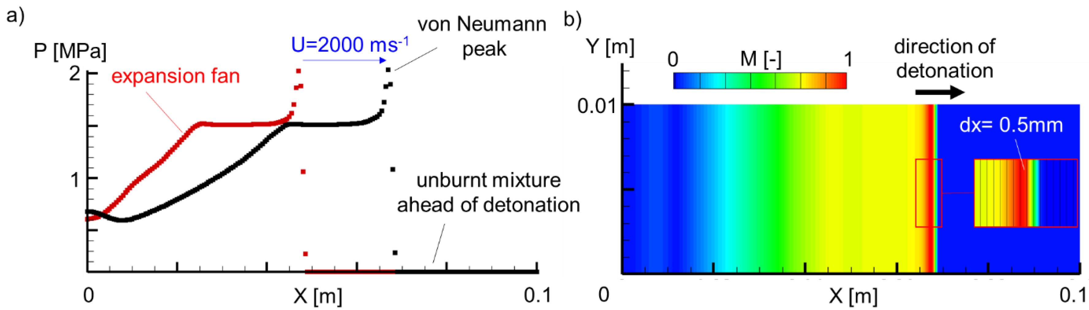
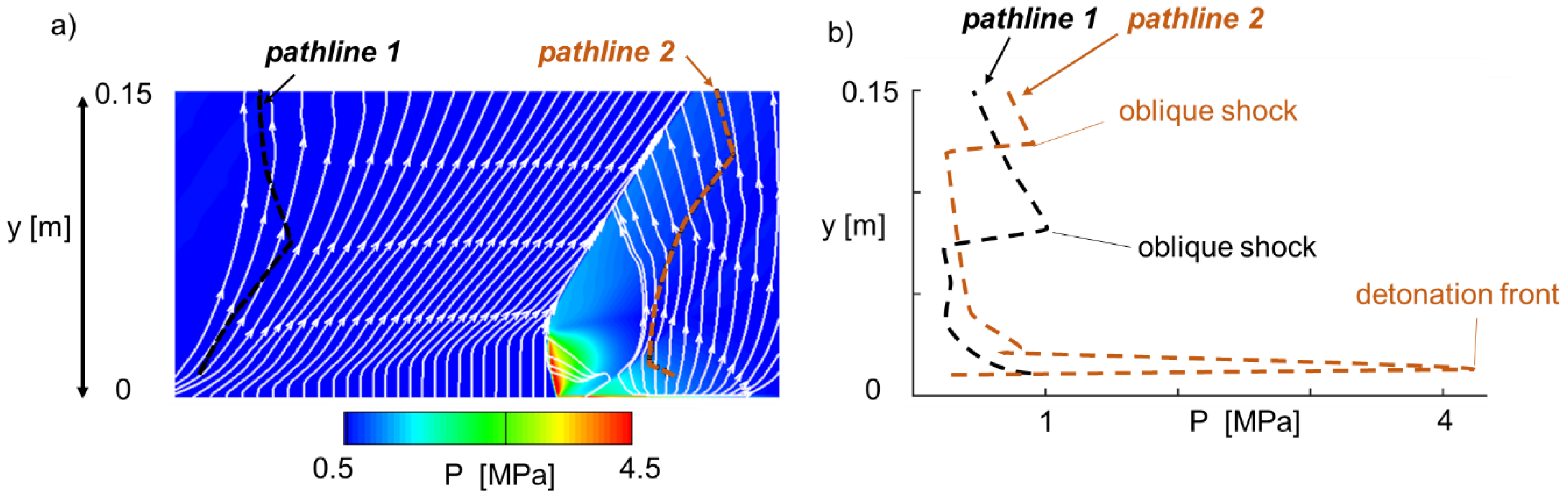
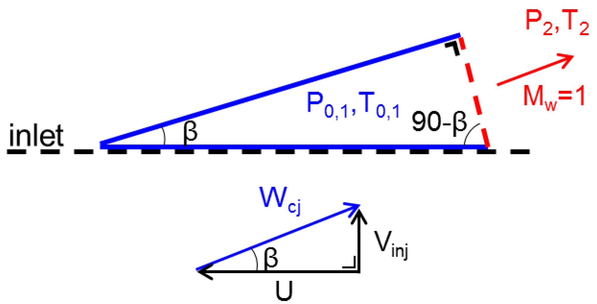
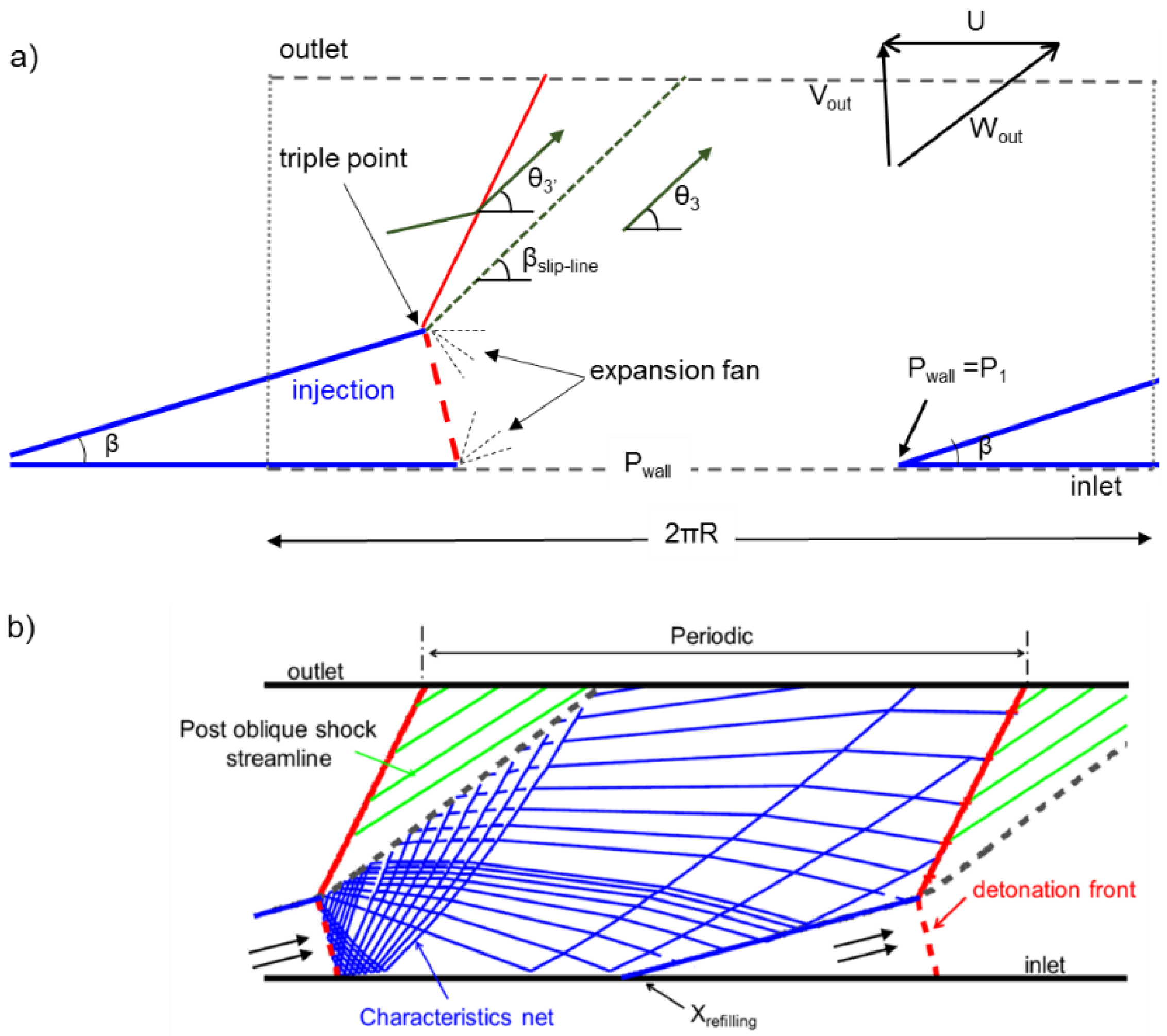
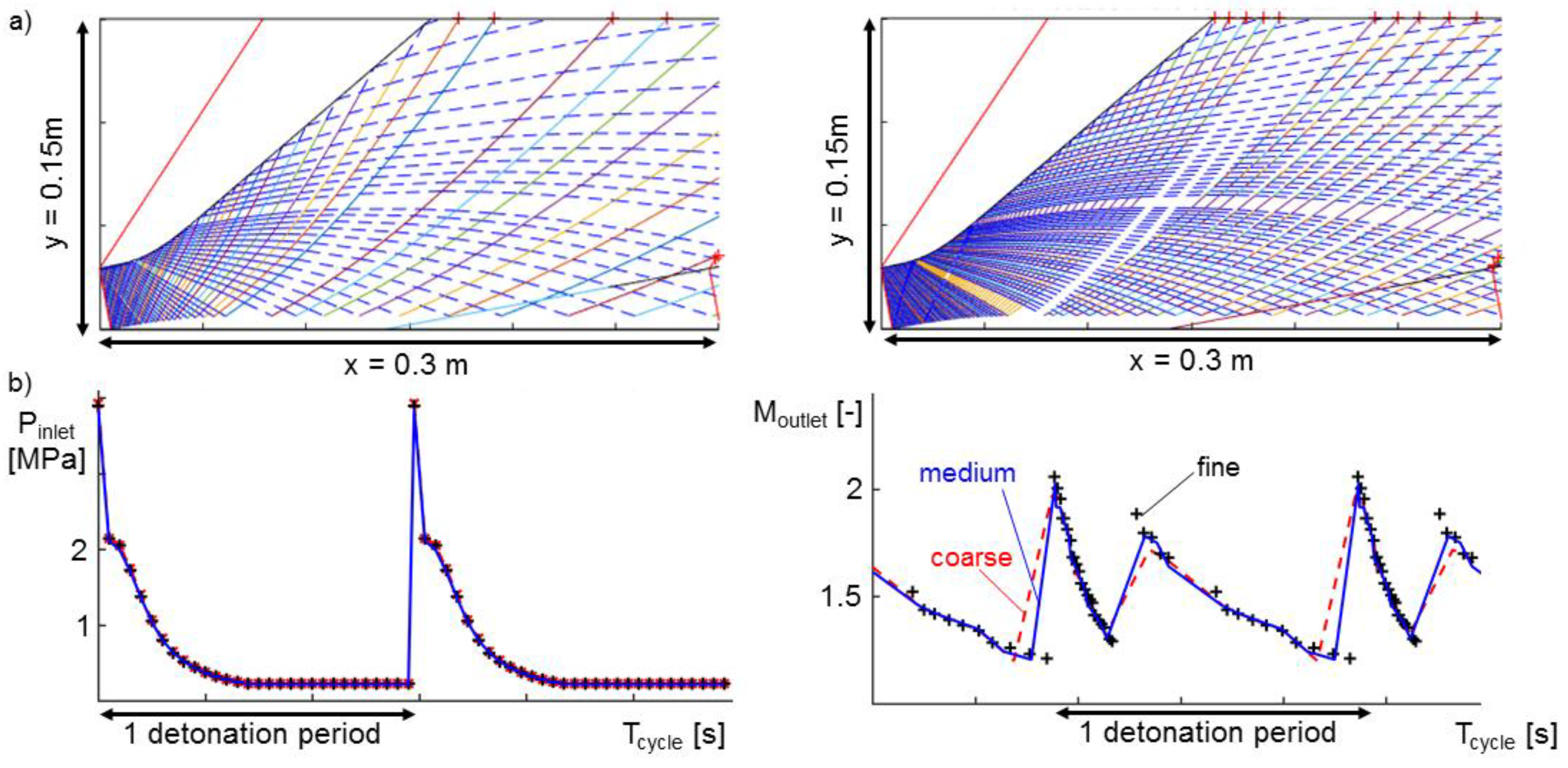
2.2. Reduced-Order Model Based on the Method of Characteristics

This section details the reduced model implementation, followed by a validation with a commercial two-dimensional URANS solver and finally a grid sensitivity of the proposed model.

The reduced-order model that we used to retrieve the flow field consists of an iterative procedure to estimate injection velocity that certifies a stable operation of the RDC [20], in a similar way to the work of Lu and Braun [29]. The flow field is solved in the relative frame of reference of the rotating shock, and the numerical procedure relies on a one-dimensional chemical solver [30] to model the detonation front. In our approach, the complete flow field is computed with a two-dimensional method of characteristics solver [31].

The initial inputs to the solver are inlet total pressure and inlet total temperature. This input (P_0,1 and T_0,1) is represented in Figure 4, which shows the triangular injection zone, where the supersonic shock moves at the velocity U, towards the swirl-free fresh reactants with velocity V_inj, a pressure P₁ and a temperature T₁. According to the velocity triangles, the relative incoming velocity (W_CJ), traveling at the Chapman–Jouguet velocity, defines the inclination of the refilling line (β) and of the detonation front. Immediately behind the detonation wave, the relative Mach number is sonic (M_w = 1) and the detonation jump conditions are computed (P₂/P₁, T₂/T₁) based on the ZND theory with the shock and detonation tool box [32]. In the present reduced-order model, both the edge of the refilling zone and the detonation front are considered to be straight lines. The edge of the refilling zone follows the same direction as the streamlines (Wcj), and the detonation wave is perpendicular to the incoming fresh mixture [20]. Therefore, the triangular zone is characterized by a 90 degree angle between the detonation wave and the edge of the refilling zone.

The model solves an unfolded rotating detonation combustor, illustrated in Figure 5a, in which a single period is represented. To analytically solve the triple point, which intersects the oblique shock wave, slip line and detonation front, continuity of pressure and flow direction (θ^’₃ = θ₃) is guaranteed across the slip line, as introduced by Sichel and Foster [33] for planar detonations. However, in rotating detonation combustors, the flow conditions just in front of the oblique shock wave are not known beforehand and need to be updated each time the solver iterates over the injection velocity. The oblique shock equations are used to retrieve the correct oblique shock-wave angle and the slip line, which ensures pressure equality. This then provides the needed boundary conditions to initiate the method of characteristics [20]. At each iteration, the pressure at the inlet wall (P_wall) is evaluated, and convergence is obtained if the pressure at the start of injection of the fresh mixture matches the injection pressure. At the end of the iterative procedure, absolute flow properties are computed for all the points. Figure 5b shows how the reduced model solves the flow field. The blue lines depict the characteristic lines from the method of characteristics, while the green lines show the oblique shock streamlines downstream of the oblique shock (in red). The reduced model needs a CPU time of 200 s on a laptop, while the 2D URANS required 40 h on 4 cores of an Intel Xeon –E5-2660 v3 processor @ 2.6 Ghz (64 GB RAM) on the RICE purdue cluster (built through a partnership with HP and Intel in April 2015 [34]).

To verify that the characteristics net is sufficiently refined, Figure 6a shows a sensitivity analysis of the characteristics net that was solved via the method of characteristics. Three simulations were selected with three different characteristic net sizes (14, 20 and 29 characteristic lines) emerging from the detonation front. Figure 6b-left shows the inlet Mach number for the three cases, and the relative error between fine and medium mesh is within 2%. Figure 6b-right shows the Mach number at the outlet of the domain, and the medium mesh shows good agreement with the fine mesh.

The accuracy of the reduced-order model was finally assessed through comparisons with the URANS results. Figure 7a depicts the total temperature evaluated with CFD++, while Figure 7b shows the results from the reduced-order model. Figure 7c shows the inlet pressure profile for four successive oblique shock traverses. The reduced-order model is able to accurately predict the onset of the refilling location as well as the speed of injection. In Figure 7d, the outlet total pressure is superimposed for both computations. There is a good agreement in the value of peak pressure, but the profile is distinct due to different expansions behind the slip zone.

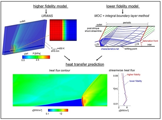
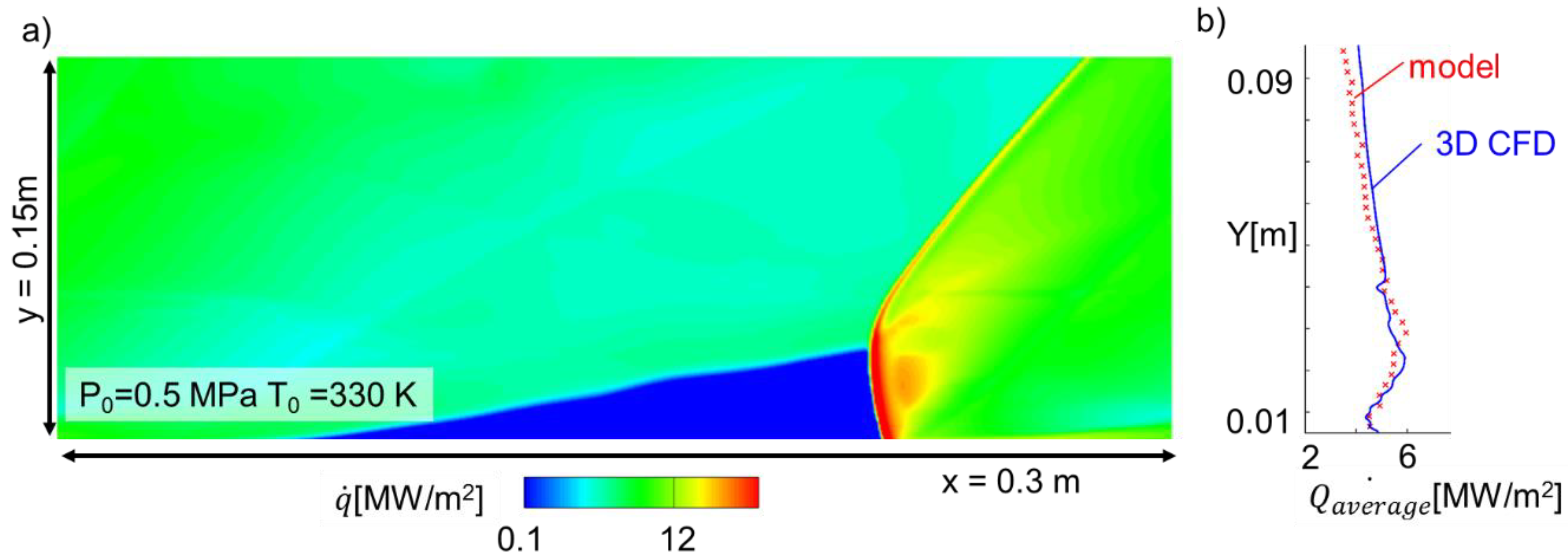
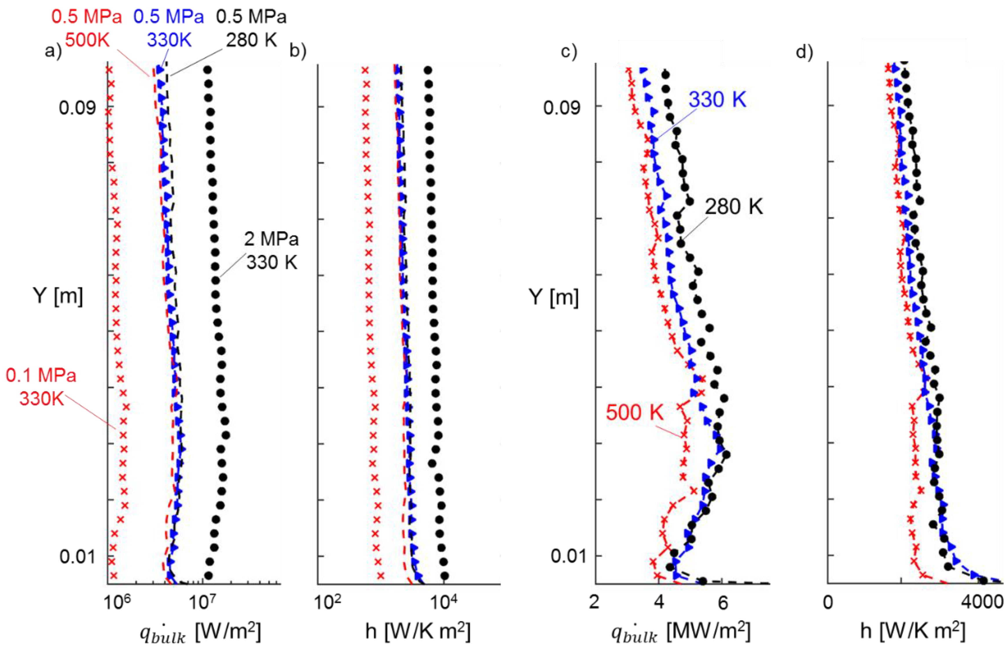
2.3. Heat-Transfer Analysis: URANS vs. Reduced-Order Model with Heat-Flux Correlation

The integral method established by Reshotko and Tucker [35] was used to compute the heat transfer between the flow boundary layer and wall, based on the estimation of the boundary layer pressure gradient from the MOC code [20]. The calculation of the aerodynamic properties of the boundary layer involves the momentum integral Equation (6) that is simplified thanks to Stewartson’s transformation for compressible flow:

$$\frac{d{\theta }_{tr}}{dx}+\frac{{\theta }_{tr}}{M_e}\frac{d{M}_e}{dx}\left(2+H_{tr}\right)=A$$

(6)

$$A=0.123e^{-1.561H_i}{\left(\frac{M_e{a}_0{\theta }_{tr}}{{\nu }_0}\right)}^{-0.268}{\left(\frac{T_e}{T_{ref}}\right)}^{0.732}{\left(\frac{T_e}{T_0}\right)}^{3.268},$$

(7)

where ${\theta }_{tr}$ is the transformed momentum thickness defined as follows:

$${\theta }_{tr}={\int }_0^{∆}\frac{U}{U_e}\left(1-\frac{U}{U_e}\right)dx.$$

(8)

If a fully developed turbulence flow is considered, Equation (8) can be integrated to predict the value of the momentum thickness at a distance x from the leading edge.

$${{\theta }_{tr}}^{1.2155}=\frac{0.01173}{{\left(\frac{a_0}{{\nu }_0}\right)}^{0.2155}{M}_e^{B+0.2155}}{\int }_0^x{M}_e^B\frac{{\left(\frac{T_e}{T_{ref}}\right)}^{0.732}}{{\left(\frac{T_0}{T_e}\right)}^{3.268}}dx,$$

(9)

where

$$B=4.2+1.2155H_{i,fp}\left(\frac{h_w}{h_0}-1\right).$$

(10)

Values with subscript e are defined at the edge of the boundary layer, while a₀ and v₀ are the speed of sound and kinematic viscosity based on the stagnation flow conditions. $H_{i,fp}$ is the incompressible form factor for a flat plate, while T_ref is evaluated at the reference enthalpy:

$$\frac{h_{ref}}{h_e}=\frac{1}{2}\left(\frac{h_w}{h_e}+1\right)+0.22\left(\frac{h_{aw}}{h_e}-1\right).$$

(11)

The adiabatic enthalpy ($h_{aw}$) is calculated as:

$$\frac{h_{aw}}{h_e}=1+\frac{\gamma -1}{2}{M}_e^2{\left(Pr\right)}_{ref}^{2/3}.$$

(12)

Finally, Reshotko and Tucker defined the Stanton number:

$$St=\frac{0.123e^{-1.151H_{i,fp}}{\left(\frac{T_e}{T_{ref}}\right)}^{0.732}}{{\left(\frac{T_0}{T_e}\right)}^{0.268}\left(\frac{M_e{a}_0{\theta }_{tr}}{{\nu }_0}\right)0.268}P{r}^{-2/3}.$$

(13)

The heat flux (q_wall) between the fluid and the wall is computed in the following way:

$$q_{wall}=St{\rho }_e{u}_e\left(h_{aw}-h_w\right).$$

(14)

A simplified numerical test case was selected to verify the accuracy of the present correlation. Figure 8a depicts the test case that comprises a two-dimensional tube with a channel height of 5 mm with a premixed H₂–air at stoichiometric conditions, with a high-pressure and high-temperature zone that ignited the combustible at the start of the simulation. The lower and upper walls were isothermal with a grid that was refined at the wall to guarantee that the viscous sublayer was well resolved. The Mach number and total conditions were measured 0.4 mm from the wall and represent the properties at the edge of the boundary layer. The wall and stagnation properties were then loaded into the model to predict the boundary layer properties to solve Equation (14) and retrieve the heat flux. Figure 8b details the heat flux on the lower wall, predicted by the URANS solver and by the correlation of Reshotko and Tucker [35]. Through this test case, the value of H_i,fp = 1.7 was set as the optimal value to correctly reproduce the heat flux peak in flows that are facing shock and detonation transients.

The dependence of the numerical accuracy with the first cell size (in terms of y+), time discretization and total number of cells was retrieved based on the Richardson extrapolation method [36]. The mesh independence study for the current manuscript was performed on a 2D mesh to determine the discretization requirements for the 3D test case. Figure 9a displays the log–log plot of the extrapolated numerical error of the maximum heat-flux level (at the shock front) as a function of the nondimensional wall distance, y+. For values of y+ smaller than 0.5, which relate to a dimensioned wall distance of 2.0 × 10⁻⁸ m, the relative error is less than 10%. On Figure 9b, the extrapolated numerical error on the maximum heat flux is shown as a function of the timestep per iteration. For values smaller than 1.0 × 10⁻⁸ s, the relative difference with regard to the 0.5 × 10⁻⁹ s case is less than 4%. For these reasons, we opted for a timestep of 1.0 × 10⁻⁸ s and a first wall distance of 2.0 × 10⁻⁸ m.

Furthermore, a grid independence study was performed to determine the grid density based on a grid convergence study [36,37]. Figure 9c plots the extrapolated convergence error for three different grid sizes. The average heat flux on the bottom plate was chosen as the key variable. To obtain a feasible calculation time with an acceptable error, the middle mesh with 60 radial grid points was chosen with an extrapolation error of 10.95%.

Finally, we applied the heat-flux methodology to our reduced-order model. First, the streamlines and the corresponding path lines were computed to track the static and the absolute stagnation conditions (Me, Te, a₀ and T₀) to retrieve the instantaneous heat flux at each spatial location via Equation (14).

2.4. Limitations of the Reduced-Order Model

The reduced-detonation-order model attempts to predict the macroscopic flow features inside the combustor, and consequently, several detailed features cannot be captured. In particular, due to the 2D assumption, local curvature is not taken into account, nor are unsteady shock-wave boundary layer interactions. Additionally, for simplicity, both the oblique shock wave and the slip line are assumed to behave as a straight line, which can slightly alter the local flow expansion after the detonation front. From the thermal analysis perspective, we assumed an isothermal wall, and therefore we neglect nonuniformities of the wall temperature. We selected the isothermal boundary conditions following the assumption that the combustor is operating under constant periodic conditions, and that the bulk wall temperature is maintained at constant temperature by the cooling system.

3. Results

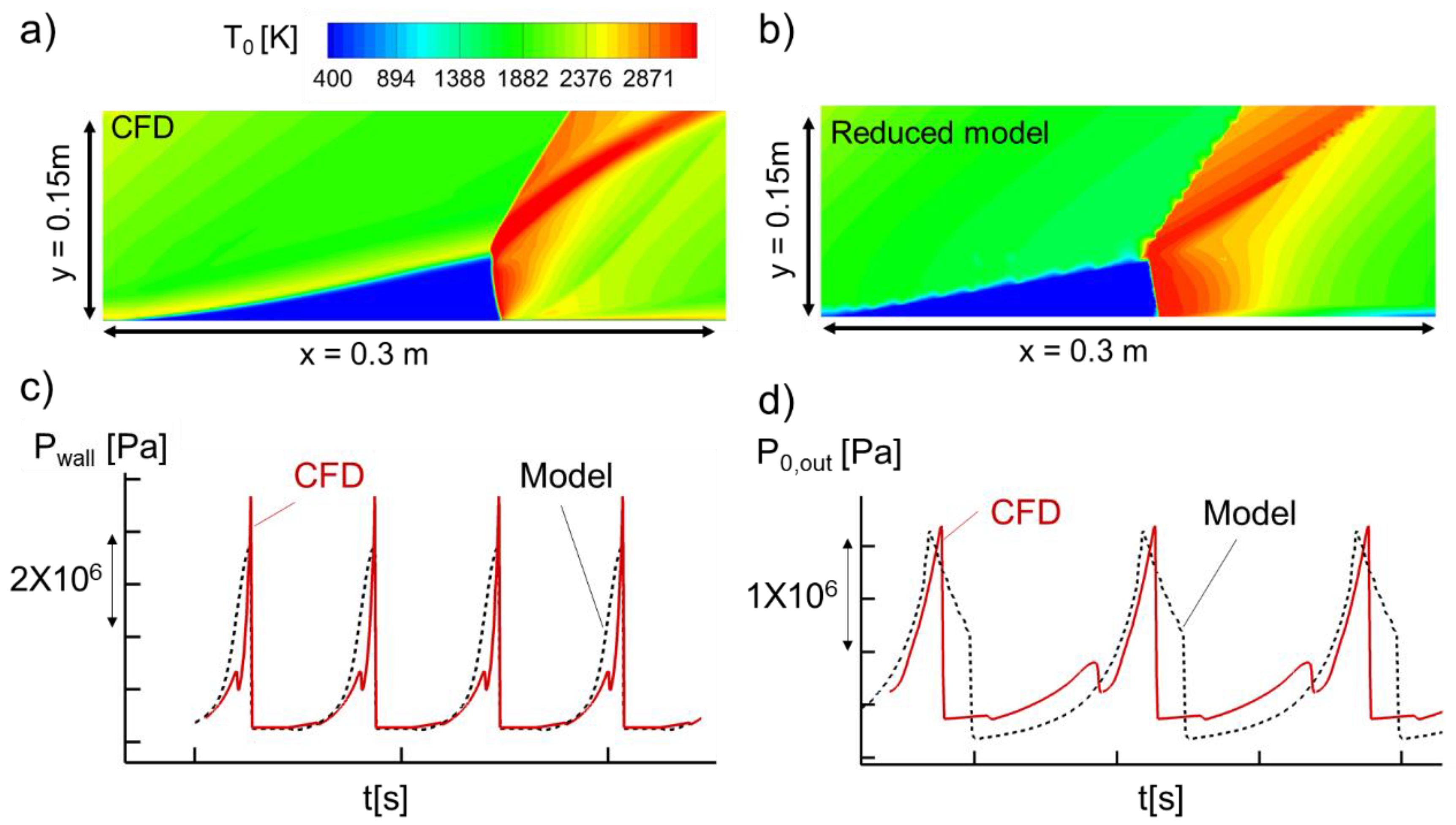
3.1. Navier–Stokes Solution vs. Reduced-Order Model

To resolve the boundary layer within the three-dimensional rotating detonation combustor, we modelled the combustor as an unrolled annulus, as shown in Figure 10a. The annulus has a thickness of 5 mm, and inlet stagnation conditions equal to 330 K and 0.5 MPa with a turbulent intensity of 5%. For this 3D simulation, turbulent equations were solved via the URANS k-omega SST model. The lateral walls were kept at a constant temperature of 450 K. The first grid point is 2.0 × 10⁻⁸ m away from the wall, to ensure a y+ below one and avoid the need for wall functions. This resulted in a three-dimensional mesh of 6.9 million cells. In order to ensure a converged result, we plot the mean heat-flux level at consecutive timesteps in Figure 10b and observe that the heat-flux fluctuation is below 0.4%. Total computational time was around 400 h on 16 cores of an Intel Xeon –E5-2660 v3 processor @ 2.6 Ghz (64 GB RAM). To speed up the computational time, the simulations were initially run on a two-dimensional mesh (described in Section 2.1 until full convergence (3.5 ms, as shown in Figure 2). Afterwards, the solution was interpolated into a 3D mesh and run for another 0.5 ms, which represented three passages of the detonation wave.

Figure 11a illustrates the iso-heat-flux contour (in logarithmic scale) at a certain timestep. At the detonation front, the peak heat flux is around 200 MW/m², followed by a smooth decrease set by the subsequent flow expansion. Since the temperature of the fresh mixture is below the wall temperature, a negative heat flux is measured during refill time of the mixture. The unsteady sweeping of the oblique shock wave augments the total temperature and total pressure, and hence increases the heat in this area. Figure 11b compares the time-averaged heat flux from both models, at different streamwise positions. Our model predicts the same level of averaged heat flux in the region of the detonation front with a maximum value up to 6 MW/m² and a decrease towards the outlet, at 0.1 m, and the model under-predicts the 3D URANS by 16%. The bulk heat flux estimated by the URANS solution is 4.8 MW/m² and 5.1 MW/m² for the reduced-order model. Interestingly, the experimental data reported in [23] shows a similar magnitude of heat flux along the axis of the combustor. The maximum bulk heat-flux variation with the 2D MOC code was about 40% (0.4 MW/m²) between the injection location and the triple point, while our 3D simulations predicted a variation of 33%.

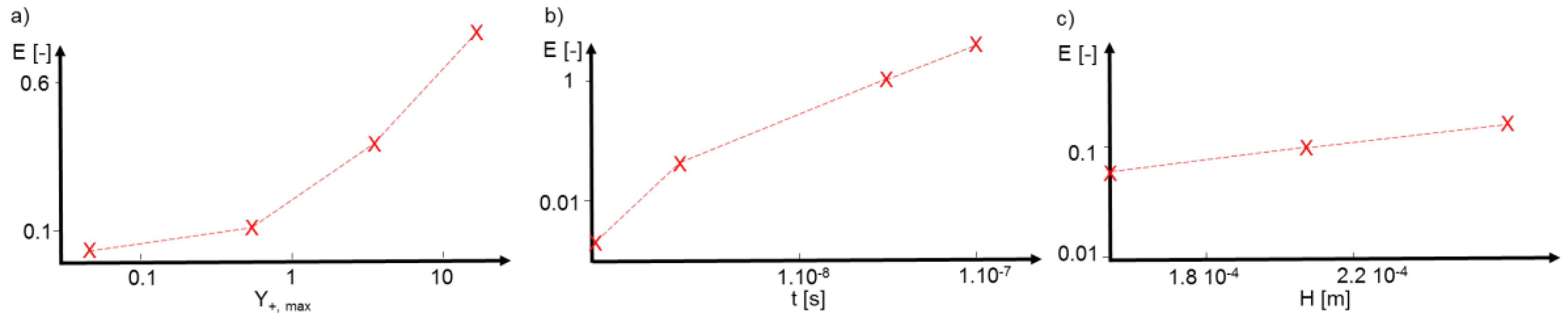
3.2. Parametric Study

The impacts of different operating conditions on heat flux and heat-transfer coefficients were examined with the reduced model. Figure 12a depicts the time-averaged heat flux along the axial direction for several inlet total pressures and inlet temperatures. When only modifying the total pressure, the change in heat flux (Figure 12b) was directly correlated with variations in the convective heat-transfer coefficient. In Figure 12c, we show the impact of changing the inlet total temperature while keeping the inlet total pressure at 0.5 MPa. The temperature variations appear to play a minor role in the overall heat-flux value (unlike the effects of pressure variations). Furthermore, when the total temperature is increased, the pressure jump across the detonation is smaller. Since this resulted in a lower total pressure with a consequent decrease in heat-transfer coefficient (Figure 12d), the heat-flux level is the lowest for the 500 K case.

4. Conclusions

This manuscript presents a fast methodology to quantify the convective heat flux in detonation combustors. The numerical approach considers the method of characteristics to compute the flow field and an integral boundary layer method to evaluate the local gas–wall heat exchange. With this tool we can estimate the average and local heat flux within the combustor at any desired operating condition. The parametric study exposed a high correlation between the convective heat-transfer coefficient and the inlet total pressure, and a lower correlation with the total inlet temperature. The model also identified the highest time-averaged heat fluxes at the location of the triple point, as equally observed in experimental data. Although the highest localized heat flux occurs all along the detonation front, this effect is then balanced by a negative heat flux from the cold fresh mixture. As a consequence, the average heat flux at the detonation-injection region is similar to the region downstream of the detonation zone. Further downstream, a slight decrease from 6 MW/m² to 4 MW/m² was observed, which agreed with existing experimental data. To evaluate the precision of the method, we performed 3D URANS on an unrolled combustor with wall refinement. The overall averaged combustor heat-flux value (5.1 MW/m²) for both methods was within 4%, but the reduced model delivered the results in seconds, several orders of magnitude faster than the three-dimensional unsteady Reynolds-averaged Navier–Stokes solver. Thanks to the limited computational time of our reduced-order model, heat-flux distribution can be estimated in a timely manner. This is essential to optimize the design of cooling schemes that can ensure the integrity of future rotating detonation combustors.

References

1. Sousa, J.; Paniagua, G.; Morata, E.C. Thermodynamic analysis of a gas turbine engine with a rotating detonation combustor. Appl. Energy 2017, 195, 247–256. [Google Scholar] [CrossRef]
2. Roy, A.; Ferguson, D.H.; Sidwell, T.; O’Meara, B.; Strakey, P.; Bedick, C.; Sisler, A. Experimental study of rotating detonation combustor performance under preheat and back pressure operation. In Proceedings of the 55th AIAA Aerospace Sciences Meeting, Grapevine, TX, USA, 9–13 January 2017; p. 1065. [Google Scholar]
3. Andrus, I.Q.; King, P.I.; Polanka, M.D.; Schauer, F.R.; Hoke, J.L. Experimentation of a premixed rotating detonation engine utilizing a variable slot feed plenum. In Proceedings of the 54th AIAA Aerospace Sciences Meeting, San Diego, CA, USA, 4–8 January 2016. [Google Scholar]
4. Anand, V.; St. George, A.; Farbos de Luzan, C.; Gutmark, E. Rotating detonation wave mechanics through ethylene-air mixtures in hollow combustors, and implications to high frequency combustion instabilities. Exp. Therm. Fluid Sci. 2018, 92, 314–325. [Google Scholar] [CrossRef]
5. Nakagami, S.; Matsuoka, K.; Kasahara, J.; Kumazawa, Y.; Fujii, J.; Matsuo, A.; Funaki, I. Experimental Visualization of the Structure of Rotating Detonation Waves in a Disk-Shaped Combustor. J. Propuls. Power 2017, 33, 80–88. [Google Scholar] [CrossRef]
6. Frolov, S.; Aksenov, V.; Ivanov, V.; Shamshin, I. Large-scale hydrogen–air continuous detonation combustor. Int. J. Hydrog. Energy 2015, 40, 1616–1623. [Google Scholar] [CrossRef]
7. Le Naour, B.; Falempin, F.H.; Coulon, K. MBDA R&T Effort Regarding Continuous Detonation Wave Engine for Propulsion—Status in 2016. In Proceedings of the 21st AIAA International Space Planes and Hypersonics Technologies Conference, International Space Planes and Hypersonic Systems and Technologies Conferences, Xiamen, China, 6–9 March 2017. [Google Scholar]
8. Davidenko, D.M.; Gokalp, I.; Kudryavtsev, A.N. Numerical study of the continuous detonation wave rocket engine. In Proceedings of the 15th AIAA International Space Planes and Hypersonic Systems and Technologies Conference, Dayton, OH, USA, 28 April–1 May 2008. [Google Scholar]
9. Zheng, H.; Qi, L.; Zhao, N.; Li, Z.; Liu, X. A Thermodynamic Analysis of the Pressure Gain of Continuously Rotating Detonation Combustor for Gas Turbine. Appl. Sci. 2018, 8, 535. [Google Scholar] [CrossRef]
10. Cocks, P.A.; Holley, A.T.; Rankin, B.A. High fidelity simulations of a non-premixed rotating detonation engine. In Proceedings of the 54th AIAA Aerospace Sciences Meeting, San Diego, CA, USA, 4–8 January 2016. [Google Scholar]
11. Frolov, S.; Dubrovskii, A.; Ivanov, V. Three-dimensional numerical simulation of operation process in rotating detonation engine. Proc. Prog. Propuls. Phys. EDP Sci. 2013, 4, 467–488. [Google Scholar]
12. Zhou, R.; Wang, J.-P. Numerical Investigation of Flow Particle Paths and Thermodynamic Performance of Continuously Rotating Detonation Engines. Combust. Flame 2012, 159, 3632–3645. [Google Scholar] [CrossRef]
13. Schwer, D.; Kailasanath, K. Numerical investigation of the physics of rotating-detonation-engines. Proc. Combust. Inst. 2011, 33, 2195–2202. [Google Scholar] [CrossRef]
14. Braun, J.; Saracoglu, B.H.; Paniagua, G. Unsteady Performance of Rotating Detonation Engines with Different Exhaust Nozzles. J. Propuls. Power 2016, 33, 121–130. [Google Scholar] [CrossRef]
15. Braun, J.; Saracoglu, B.H.; Magin, T.E.; Paniagua, G. One-Dimensional Analysis of the Magnetohydrodynamic Effect in Rotating Detonation Combustors. AIAA J. 2016, 54, 3761–3767. [Google Scholar] [CrossRef]
16. Ornano, F.; Braun, J.; Saracoglu, B.H.; Paniagua, G. Multi-stage nozzle-shape optimization for pulsed hydrogen–air detonation combustor. Adv. Mech. Eng. 2017, 9, 1–9. [Google Scholar] [CrossRef]
17. Eude, Y.; Davidenko, D.M.; Gokalp, I.; Falempin, F. Use of the adaptive mesh refinement for 3D simulations of a CDWRE (continuous detonation wave rocket engine). In Proceedings of the 17th AIAA International Space Planes and Hypersonic Systems and Technologies Conference, San Francisco, CA, USA, 13 April 2011. [Google Scholar]
18. Mizener, A.R.; Lu, F.K. Low-Order Parametric Analysis of a Rotating Detonation Engine in Rocket Mode. J. Propuls. Power 2017, 33, 1543–1554. [Google Scholar] [CrossRef]
19. Fievisohn, R.T.; Yu, K.H. Steady-State Analysis of Rotating Detonation Engine Flow fields with the Method of Characteristics. J. Propuls. Power 2016, 33, 89–99. [Google Scholar] [CrossRef]
20. Sousa, J.; Braun, J.; Paniagua, G. Development of a fast evaluation tool for rotating detonation combustors. Appl. Math. Model. 2017, 52, 42–52. [Google Scholar] [CrossRef]
21. Roy, A.; Bedick, C.; Strakey, P.; Sidwell, T.; Ferguson, D.; Sisler, A.; Nix, A. Development of a Three-dimensional Transient Wall Heat Transfer Model of a Rotating Detonation Combustor. In Proceedings of the 54th AIAA Aerospace Sciences Meeting, San Diego, CA, USA, 4–8 January 2016. [Google Scholar]
22. Olcucuoglu, B.; Temel, O.; Tuncer, O.; Saracoglu, B.H. A Novel Open Source Conjugate Heat Transfer Solver for Detonation Engine Simulations. In Proceedings of the AIAA Aerospace Sciences Meeting, AIAA SciTech Forum, Kissimmee, FL, USA, 12 January 2018. [Google Scholar]
23. Theuerkauf, S.W.; Schauer, F.; Anthony, R.; Hoke, J. Experimental Characterization of High-Frequency Heat Flux in a Rotating Detonation Engine. In Proceedings of the 53rd AIAA Aerospace Sciences Meeting, Kissimmee, FL, USA, 5–9 January 2015. [Google Scholar]
24. Meyer, S.J.; Polanka, M.D.; Schauer, F.R.; Hoke, J.L. Parameter impact on heat flux in a rotating detonation engine. In Proceedings of the 2018 AIAA Aerospace Sciences Meeting, AIAA SciTech Forum, Kissimmee, FL, USA, 12 January 2018. [Google Scholar]
25. Chakravarthy, S.; Peroomian, O.; Goldberg, U.; Palaniswamy, S. The CFD++ Computational Fluid Dynamics Software Suite. In Proceedings of the AIAA and SAE, World Aviation Conference, Anaheim, CA, USA, 28–30 September 1998. [Google Scholar]
26. McBride, B.J.; Gordon, S.; Reno, M. Thermodynamic Data for Fifty Reference Elements; NASA Technical Memorandum 3287/REV1; National Aeronautics and Space Administration: Washington, DC, USA, 2001.
27. Sousa, J.; Paniagua, G.; Saavedra, J. Aerodynamic response of internal passages to pulsating inlet supersonic conditions. Comput. Fluids 2017, 149, 31–40. [Google Scholar] [CrossRef]
28. Towery, C.A.; Smith, K.M.; Shrestha, P.; Hamlington, P.E.; Van Schoor, M. Examination of Turbulent Flow Effects in Rotating Detonation Engines. In Proceedings of the 44th AIAA Fluid Dynamics Conference, San Diego, CA, USA, 16–20 June 2014. [Google Scholar]
29. Lu, F.K.; Braun, E.M. Rotating detonation wave propulsion: Experimental challenges, modeling, and engine concepts. J. Propuls. Power 2014, 30, 1125–1142. [Google Scholar] [CrossRef]
30. Goodwin, D.G.; Moffat, H.K.; Speth, R.L. Cantera: An Object-Oriented Software Toolkit for Chemical Kinetics, Thermodynamics and Transport Processes. Version 2.2.1. 2016. Available online: http://code.google.com/p/cantera (accessed on 22 May 2018).
31. Sousa, J.; Paniagua, G. Entropy Minimization Design Approach of Supersonic Internal Passages. Entropy 2015, 17, 5593–5610. [Google Scholar] [CrossRef]
32. Browne, S.; Ziegler, J.; Shepherd, J.E. Numerical Solution Methods for Shock and Detonation Jump Conditions; GALCIT Report FM2006.006; GALCIT: San Diego, CA, USA, 2004. [Google Scholar]
33. Sichel, M.; Foster, J. The ground impulse generated by a plane fuel-air explosion with side relief. Acta Astronaut. 1979, 6, 243–256. [Google Scholar] [CrossRef]
34. Rice Purdue Community Cluster. Available online: https://www.rcac.purdue.edu/compute/rice (accessed on 22 May 2018).
35. Reshotko, E.; Tucker, M. Approximate Calculation of the Compressible Turbulent Boundary Layer with Heat Transfer and Arbitrary Pressure Gradient; NACA Technical Note 4154; NACA: Boston, MA, USA, 1957. [Google Scholar]
36. Celik, I.B.; Ghia, U.; Roache, P.J. Procedure for estimation and reporting of uncertainty due to discretization in CFD applications. J. Fluids Eng.-Trans. ASME 2008, 130. [Google Scholar] [CrossRef]
37. Bonfiglioli, A.; Paciorri, R. Convergence Analysis of Shock-Capturing and Shock-Fitting Solutions on Unstructured Grids. AIAA J. 2014, 52, 1404–1416. [Google Scholar] [CrossRef]
38. Braun, J.; Sousa, J.; Paniagua, G. Assessment of the Boundary Layer within a Rotating Detonation Combustor. In Proceedings of the AIAA Propulsion and Energy Forum and Exposition, Salt Lake City, UT, USA, 25–27 July 2016. [Google Scholar]
Figure 1. (a) Verification of detonation on 1D detonation tube with pressure distribution. (b) Mach contour.
Applsci 08 00893 g001
Figure 2. (a) Iso-temperature contour of the rotating detonation combustor (RDC). (b) Pressure-gain coefficient as a function of time.
Applsci 08 00893 g002
Figure 3. (a) Instantaneous streamlines (in white) used to compute the two pathlines. (b) Pressure evolution for two selected pathlines.
Applsci 08 00893 g003
Figure 4. Refilling zone (top) with the representation of the velocity triangles and filling angle β (bottom).
Applsci 08 00893 g004
Figure 5. (a) View of the flow features within the unrolled RDC; (b) characteristic net of the model.
Applsci 08 00893 g005
Figure 6. (a) Characteristic net for the coarse and fine simulation. (b) Inlet pressure and outlet Mach number for the coarse, medium and fine mesh.
Applsci 08 00893 g006
Figure 7. Total temperature contour for (a) unsteady Reynolds Averaged Navier Stokes (URANS) simulation and (b) reduced-order model; comparison between both methods for: (c) static inlet pressure and (d) total outlet pressure.
Applsci 08 00893 g007
Figure 8. (a) 2D detonation tube: pressure flow field; (b) wall heat-flux evolution with 2D URANS vs prediction based on the correlation [18].
Applsci 08 00893 g008
Figure 9. (a) The log–log plot of the numerical extrapolated error as a function of the first-layer wall thickness; (b) log–log plot of the numerical error as a function of the timestep; (c) log–log plot of the extrapolated numerical error in terms of the characteristic mesh size H.
Applsci 08 00893 g009
Figure 10. (a) Numerical domain with mesh refinement close to the boundary layer. (b) Mean time-averaged heat-flux evolution as a function of time.
Applsci 08 00893 g010
Figure 11. (a) Wall heat-flux contour (3D URANS solution). (b) Comparison of the averaged heat flux computed with the reduced-order model and 3D URANS simulation.
Applsci 08 00893 g011
Figure 12. Time-averaged heat flux and heat-transfer coefficient in the streamwise direction with the reduced-order model for different inlet total pressures and total temperatures (a,b); and a detailed view showing the impact of different inlet total temperatures (c,d).
Applsci 08 00893 g012