Article

A Simplified Free Vortex Wake Model of Wind Turbines for Axial Steady Conditions

1
College of Energy and Electrical Engineering, Hohai University, Nanjing 211100, China
2
Jiangsu Key Laboratory of Hi-Tech Research for Wind Turbine Design, Nanjing University of Aeronautics and Astronautics, Nanjing 210016, China
*
Author to whom correspondence should be addressed.
Appl. Sci. 2018, 8(6), 866; https://doi.org/10.3390/app8060866
Submission received: 18 April 2018 / Revised: 20 May 2018 / Accepted: 22 May 2018 / Published: 25 May 2018
(This article belongs to the Special Issue Wind Turbine Aerodynamics)

Abstract

:
A simplified free vortex wake (FVW) model called the vortex sheet and ring wake (VSRW) model was developed to rapidly calculate the aerodynamic performance of wind turbines under axial steady conditions. The wake in the simplified FVW model is comprised of the vortex sheets in the near wake and the vortex rings, which are used to replace the helical tip vortex filament in the far wake. The position of the vortex ring is obtained by the motion equation of its control point. Analytical formulas of the velocity induced by the vortex ring were introduced to reduce the computational time of the induced velocity calculation. In order to take into account both accuracy and calculation time of the VSRW model, the length of the near wake was cut off at a 120° wake age angle. The simplified FVW model was used to calculate the aerodynamic load of the blade and the wake flow characteristic. The results were compared with measurement results and the results from the full vortex sheet wake model and the tip vortex wake model. The computational speed of the simplified FVW model is at least an order of magnitude faster than other two conventional models. The error of the low-speed shaft torque obtained from the simplified FVW model is no more than 10% relative to the experiment at most of wind speeds. The normal and tangential force coefficients obtained from the three models agree well with each other and with the measurement results at the low wind speed. The comparison indicates that the simplified FVW model predicts the aerodynamic load accurately and greatly reduces the computational time. The axial induction factor field in the near wake agrees well with the other two FVW models and the radial expansion deformation of the wake can be captured.

1. Introduction

Over the past four decades, free vortex wake (FVW) methods have emerged as robust and versatile tools for modeling the aerodynamic performance of wind turbine rotors. Unlike the blade element momentum (BEM) theory [1,2] where annular average induction is found, the FVW method can determine vortical induction directly at the blade elements from the effect of the modeled wake and the method is more efficient than computational fluid dynamic (CFD) methods. However, the computational cost of the FVW method is much higher than that of the BEM method. Perhaps this is the reason that the FVW method is not commonly used for predicting the aerodynamic loads of wind turbine rotors in the wind energy community.
FVW methods are based on a discrete representation of the rotor vorticity field and a Lagrangian representation of the governing equations for the wake elements. In essence, the wake elements are allowed to convert and deform under the action of the local velocity field to force-free locations. Clearly, the ability to predict the aerodynamic performance of wind turbines is strongly dependent on the ability to predict the highly complex wake geometry. Free wake analyses are fundamentally better suited to the complex flowfields generated by wind turbines and avoid the difficulty of prescribing a wake geometry but, in so doing, introduce more computational costs. Gohard [3] presented the first full vortex sheet wake (FVSW) model for horizontal axis wind turbines, in which the unconstrained wake was permitted to move freely with the local velocities existing in the wake. The initial wake geometry of the FVSW model is shown in Figure 1a. FVSW methods for the analysis of wind turbine aerodynamics were also used by Arsuffi et al. [4], Garrel [5], Sant et al. [6] and Sebastian et al. [7]. These methods are computationally expensive, making them somewhat impractical as a design tool. To remedy this problem, Rosen et al. [8] divided the wake into two regions, i.e., near and far wakes. The calculations associated with the far wake are speeded up by some approximations. The most popular approximation is the tip vortex wake (TVW) model [9,10,11,12] as shown in Figure 1b, in which, the far wake extends beyond the near wake and is comprised of a single helical tip vortex filament, which is appropriate based on the physics of the flow. The strength of the tip vortex is determined by assuming that the sum of the blade bound vorticity outside of the maximum is trailed into the tip vortex. The release point of the tip vortex is usually the tip of the blade. More significant simplifications to the FVW models for wind turbines are attributed to Miller [13], Afjeh et al. [14], and Yu et al. [15]. The vortex wake system was simplified by Miller [13] and Afjeh et al. [14] into three parts: a number of straight semi-infinite vortex lines, a series of vortex rings, and a semi-infinite vortex cylinder. The method has been used for comprehensive rotorcraft and wind turbine analyses. Yu et al. [15] developed a free wake model that combines a vortex ring model with a semi-infinite cylindrical vortex tube, in which the thrust coefficient of the rotor must be known and is used to calculate the strength of the new vortex ring produced in a time step. Except for the approximations of the wake, parallelization techniques have been used to address the computational expense problem of the FVW model. Farrugia et al. [16] modified the FVW code Wake Induced Dynamics Simulator (WInDS) [7] to enable parallel processing. Later, Elgammi et al. [17] used the modified model to investigate the cycle-to-cycle variations in the aerodynamic blade loads experienced by yawed wind turbine rotors operating at a constant speed with a fixed yaw angle. Turkal et al. [18] used a Graphics Processing Unit (GPU), to exploit the computational parallelism involved in the free-wake methodology.
In FVW methods, the number of discrete elements per vortex filament can be very large, making the tracking process memory-intensive and computationally demanding, although still considerably less demanding than when using CFD methods. The FVSW model has a computation time of about tens of minutes at one steady condition, and the TVW model has a computation time of about several minutes. Although the TVW model requires much less computational time than the FVSW model because it has fewer wake nodes in the far wake, the computational cost makes it somewhat impractical as an iterative optimization design tool. The main objective of this study is to reduce the number of wake nodes that need to be computed and achieve lower computation time in the axial steady condition. The velocity in the plane of rotation of the blade induced by the near wake is remarkable, so the near wake is still modeled by the vortex sheets in order to reflect the actual flow in this study. The effect of the far wake on the plane of rotation is relatively smaller due to the increase in distance, so the far wake is simplified into a series of vortex rings through learning from the studies of Miller [13] and Yu et al. [15]. Therefore, the new simplified FVW model is referred to as the vortex sheet and ring wake (VSRW) model.
In Section 2, the development of the VSRW model is described. Section 3 describes the analysis of the effect of the length of the near wake. The results are presented in Section 4 and include the rate of convergence of the wake iteration, the wake geometry, the induction factor in the wake, and the low-speed shaft torque (LSST). The conclusions are drawn in Section 5.

2. Simplified Free Vortex Wake
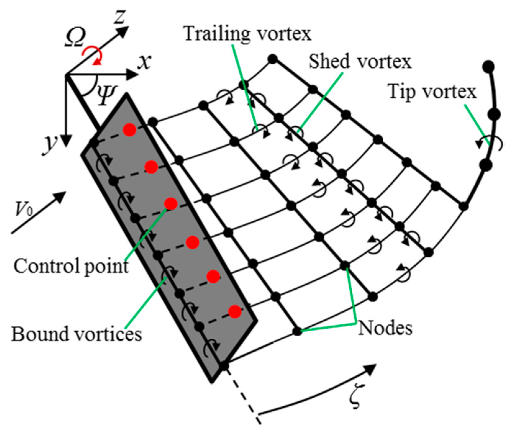
The development of the simplified FVW model will be presented in this section. The blade model is first briefly introduced and then the representation of the wake model is provided, including the near wake model and the far wake model. For completeness, the calculation procedure of the simplified FVW model is detailed.

2.1. Blade Model

The FVW model assumes that the flow field is incompressible and potential. Figure 2 shows the rotor body frame coordinates with the z-axis pointing downstream. The blade is modeled by the Weissinger-L model [19], which is a good compromise between the lifting line and the lifting surface models, as a series of straight constant-strength vortex segments lying along the blade quarter chord line. The control points are located at the 3/4-chord line at the center of each vortex segment. The wake vortices extend downstream from the 1/4-chord and form a series of horseshoe filaments. The trailing and shed vortices are modeled by the trailing and shed straight-line vortex filaments as shown in Figure 2.
The blade root section corresponds to the boundary of the first blade element. The remaining boundary distribution along each blade is achieved using the following “arc-cosine” relationship:
( r ¯ b ) i = ( r b ) i R = 2 π arccos ( 1 i 1 N E )
where NE is the number of blade elements and i is the element boundary number (i = 1, …, NE + 1). Consequently, there are NE element control points and (NE + 1) boundary points.
The strength, Γb, of each blade element is evaluated by the application of the Kutta-Joukowski theorem on the basis of airfoil data. The bound vorticity for the ith blade element is given by:
( Γ b ) i = 1 2 W i C l c i
where Wi is the resultant velocity at the ith control point and ci is the chord of the ith blade element. To take into account the three-dimensional rotational effect, the 2D airfoil data is modified by the Du-Selig stall-delay model [20].

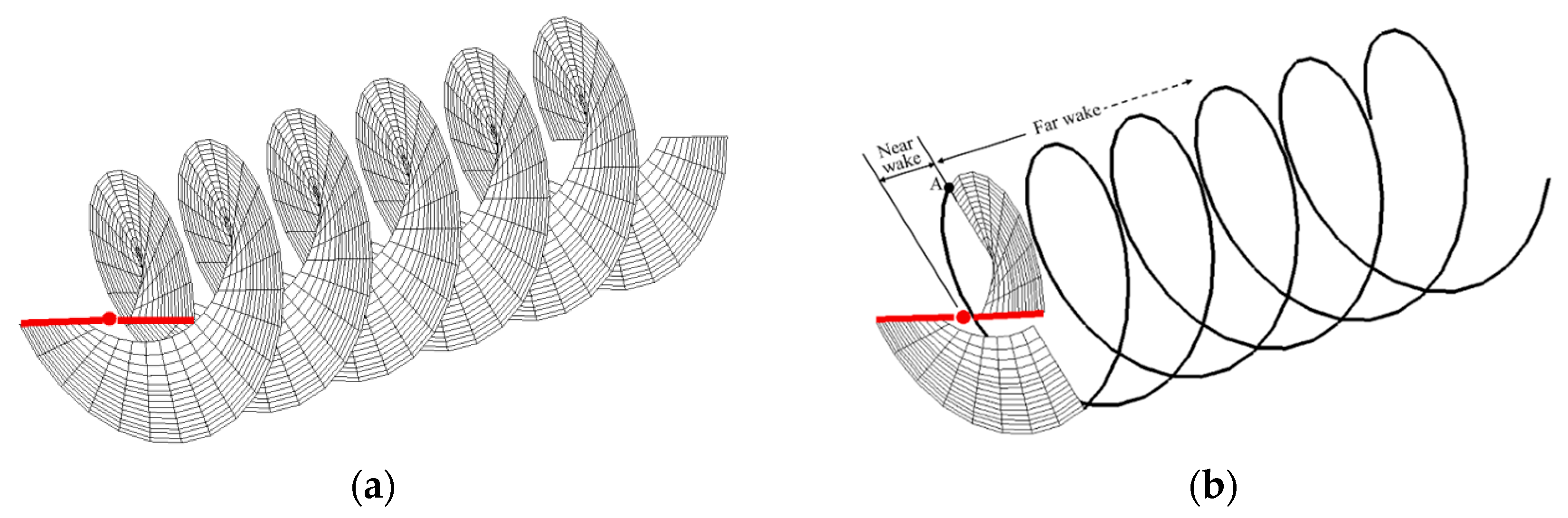
2.2. Near Wake Model

The wake that extends downstream from the blade is divided into two parts: the near wake and the far wake (Figure 1b). The near wake is modeled by the vortex sheets, which consist of the trailing and shed vortex filaments. The circulation of each blade element is assumed to be constant. However, the adjacent segments may have unequal loadings and, therefore, have different circulation strengths. The circulation strength of each trailing vortex is equal to the difference between the bound vortex strengths of the two adjacent segments. The circulation strength of each shed vortex is equal to 0 in the axial steady condition. The vortex filaments are allowed to freely distort under the influence of the local velocity field. The convection of these vortex filaments can be described by the Helmholtz equation. For a blade with fixed coordinates, the governing equation of the vortex filaments can be written as the partial differential form:
r v ( ψ , ζ ) ψ + r v ( ψ , ζ ) ζ = 1 Ω [ V 0 + V i n d ( ψ , ζ ) ]
where r is the position vector of the vortex collocation point; Vind equals the mean value of the induced velocities at the surrounding four grid points [9].
To solve the convection equation of the vortex filaments, numerical solutions have been investigated over the last decades, including relaxation methods [21] and time-marching methods [9,11]. The time-marching methods can potentially provide the best level of approximation to the rotor wake problem with the fewest application restrictions. However, these methods have been found to be rather susceptible to numerical instabilities [22]. On the other hand, the relaxation methods improve the ability to control the non-physical wake instabilities by explicit enforcement of the wake periodicity. The relaxation methods can only be used for steady-state problems.
In this study, the axial steady conditions are predicted. It is sufficient to apply a steady relaxation scheme to solve the convection equation of the vortex filaments in the near wake. A five-point central difference approximation is used for both the temporal and spatial derivatives. The detailed information can be found in Reference [21]. A pseudo-implicit technique [23,24] has been introduced to improve the stability of the free-vortex iteration. The effective range of the azimuthal discretization is usually between Δ ψ = 5° and Δ ψ = 20° [22,25] and Δ ψ = 10° was selected for use in this study. The spatial step Δ ζ uses the same value as the azimuthal step.
The velocity in the plane of rotation of the blade induced by the near wake is remarkable, so the length of the near wake is significant for the accuracy of the proposed model. The determination of the length of the near wake will be discussed further in Section 3.

2.3. Far Wake Model

In the TVW model, the far wake is modeled by the tip vortex model. In this study, vortex rings are used to replace the helical tip vortex filament as shown in Figure 3. Point A is the release point of the tip vortex and point C is the origin point of the 2nd circular tip vortex filament. The intersection point B of the vortex ring and the replaced helical tip vortex filament is located at the middle of every circular helical filament. The center of the ring is on the rotor’s rotation axis. The point 1 opposite the point B on the ring is the control point of the vortex ring. The wake length in this paper is 4R. The number of the vortex rings is determined by the wake length:
N C = INT ( 4 R V 0 Ω 2 π ) + 1
where the equation INT is an integer-valued function; therefore, we need to add 1 to consider the missing part.
As shown in Figure 3, points 1, 2, and 3 are the control points of the 1st, 2nd, and 3rd vortex rings respectively. In the axial steady condition, the vortex rings in the far wake are stationary when the wake geometry is convergent. It is assumed that point A will arrive at the position of point 1 when it moves under the influence of the velocity of point A for one half of the rotational period. Therefore, one period will be experienced between the two control points of the adjacent vortex rings. The position of the nth control point can be represented by its axial position Z c r ( n ) and its radial position R c r ( n ) . The axial position can be obtained by:
Z c r ( 1 ) = Z A + k = 1 N T / 2 Δ ψ Ω ( V 0 + V i n d , Z A ) Z c r ( n ) = Z c r ( n - 1 ) + k = 1 N T Δ ψ Ω ( V 0 + V i n d , Z n 1 ) , 2 n N C
The radial position can be obtained by:
R c r ( 1 ) = R A + k = 1 N T / 2 Δ ψ Ω V i n d , R A R c r ( n ) = R c r ( n - 1 ) + k = 1 N T Δ ψ Ω V i n d , R n 1 , 2 n N C

2.4. Velocity Induced by the Near Wake and the Far Wake

2.4.1. Velocity Induced by the Near Wake

The vortex filaments of the near wake comprise a series of straight-line vortex elements. The velocity induced by the vortex filaments equals the sum of the velocities induced by the straight-line vortex elements at the control nodes of the vortex elements, which are calculated using the Biot–Savart law as:
V i n d = Γ 4 π h ( cos θ A cos θ B ) r A × r B | r A × r B |
where h, θA, θB, rA, and rB are as shown in Figure 4. However, if a collocation point is positioned very close to the vortex-line segment, then ( h 0 ) will result in a very high induced velocity. In addition, the self-induced velocity ( h = 0 ) exhibits a logarithmic singularity. These two phenomena cause convergence problems. To avoid these numerical problems, some vortex core models based on the Lamb-Oseen vortex model [26], Ramasamy and Leishman vortex model [27], Vatistas vortex model [28] and β-Vatistas vortex model [29,30] have been applied in a FVW model. In our recent work, we compared the effects of the β-Vatistas model and Lamb-Oseen model in the FVW model [29] and further studied the application [30] of the β-Vatistas model. In this study, a vortex core model based on the Lamb-Oseen vortex model, which is the most widely adopted and simpler model, was used. To account for the effect of viscous diffusion, the vortex core radius growth is used in the Biot-Savart law and is modified by using an empirical viscous growth model [31]. The stretching effect of the vortex filaments is taken into account by the application of a model developed by Ananthan and Leishman [32].

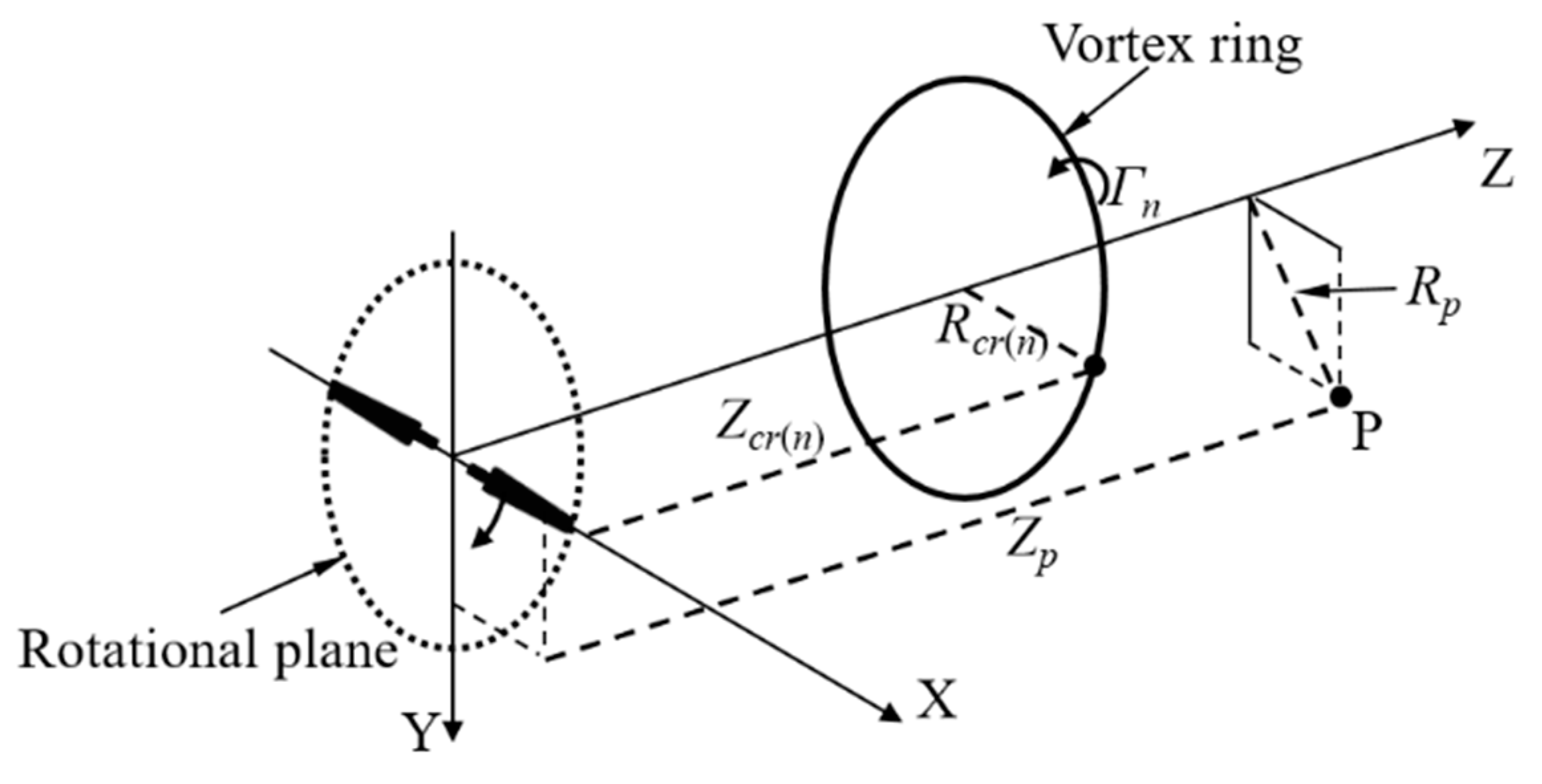
2.4.2. Velocity Induced by the Far Wake

The analytical formulas of the velocity induced by a vortex ring are given by Yoon and Heister [33]. Figure 5 shows the Cartesian coordinate system used in this study for the induced velocity calculation. The axial and radial velocities at an arbitrary point P induced by the nth vortex ring are given by:
v i n d , z = Γ n 2 π a [ K ( m ) b 2 + R p 2 R c r ( n ) 2 a 2 4 R p R c r ( n ) E ( m ) ]
v i n d , r = b Γ n 2 π R p a [ K ( m ) b 2 + R p 2 + R c r ( n ) 2 a 2 4 R p R c r ( n ) E ( m ) ]
where
a = ( Z p Z c r ( n ) ) 2 + ( R p + R c r ( n ) ) 2
b = Z p Z c r ( n )
K ( m ) and E ( m ) are the complete elliptic integrals of the first and second kind, where m is given by:
m = 4 R p R c r ( n ) a 2
A fast method [34] is used for evaluating the first and second integrals. When point P is on the vortex ring, the induced velocity is calculated by Equation (7) to avoid the self-induced numerical problem.

2.5. Calculation Procedure

The calculation process of the proposed simplified FVW model is shown in Figure 6. The following provides detailed explanations for some steps in the flowchart.
  • In step 2, the initial wake geometry of the near wake consists of a set of regular helixes. The initial wake geometry of the far wake is calculated by Equations (5) and (6) and the initial induced velocities in the two equations equal 0.
  • In step 5 and step 7, the velocity at the node and the control point induced by the vortices is calculated using the methods in Section 2.4.
  • In step 6, the five-point central difference approximation is used to solve the convection equation of the vortex filaments in the near wake and Equations (5) and (6) are used to obtain the shape and location of the vortex rings in the far wake.
  • In step 8, the root mean square (RMS) change between the new wake geometry and the old wake geometry of the two iteration steps is calculated. If the RMS change is less than a prescribed tolerance of 10−4, convergence is achieved. Otherwise, return to step 3.

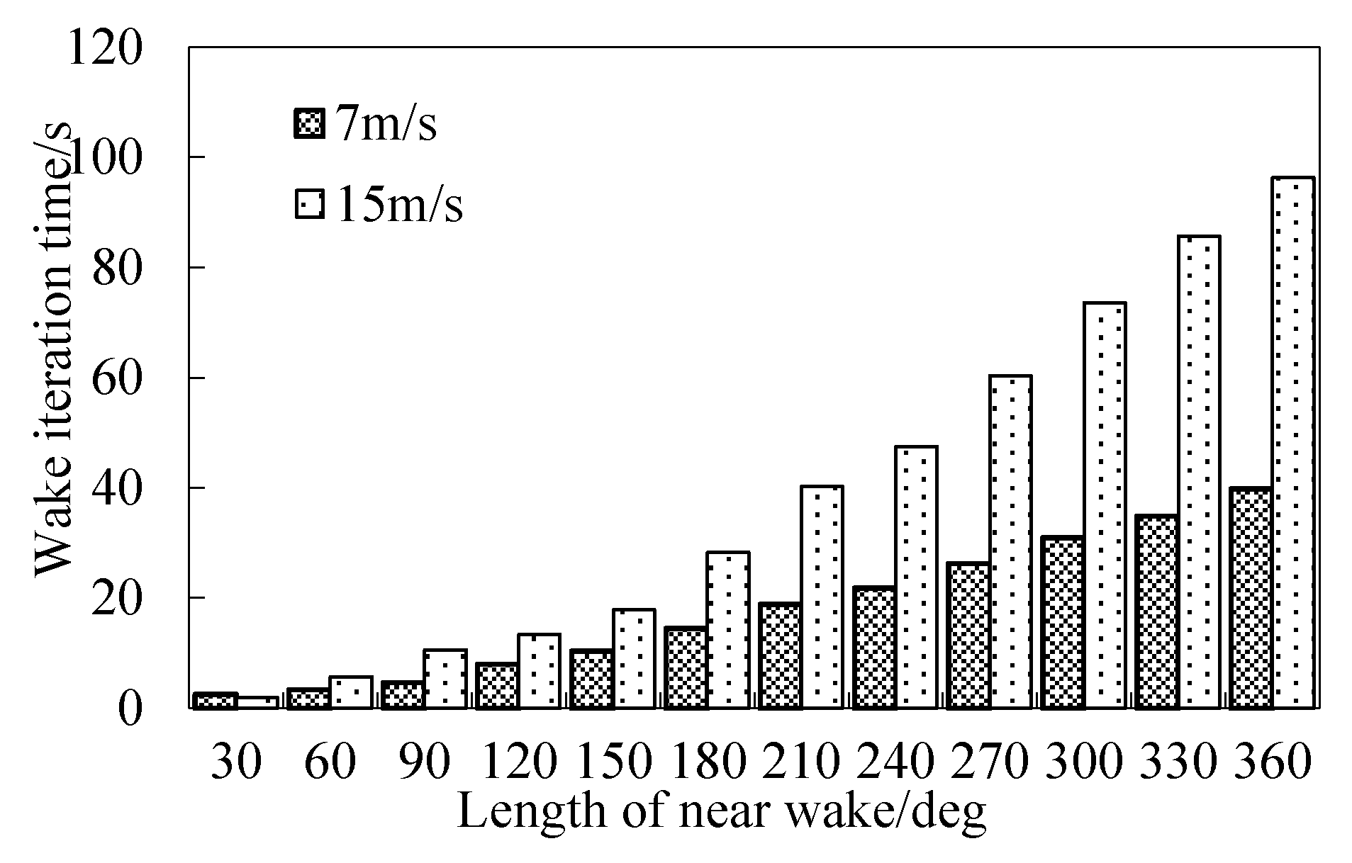
3. Length of Near Wake

To validate the VSRW model, the National Renewable Energy Laboratory (NREL) Phase VI wind turbine is used in this paper as a test case. The NREL Phase VI is a stall-regulated turbine. This turbine was designed by the NREL. The experiments were performed in the National Aeronautics and Space Administration (NASA) Ames wind tunnel (24.4 × 36.6 m) [35], which is considered a benchmark for the evaluation of wind turbine aerodynamic methods.
In the TVW model, the near wake is truncated after a short azimuthal distance, which is typically an azimuth angle of about 60° [36] in the helicopter field. Beyond this point, the far wake extends and is comprised of a single tip vortex filament. In the proposed VSRW model, one should ensure that the vortex sheet extends sufficiently far downstream. The aerodynamic performance of the rotor should be independent of the length of the vortex sheet. The length of the vortex sheet (or length of the near wake) can be represented by the wake age angle of the near wake. The spatial step equals 10° as mentioned above.
The LSST has been calculated used different lengths of the near wake ranging from 10° to 360°. Figure 7 shows the LSST along the length of the near wake at different wind speeds. As the length of the near wake increases from 10°, the LSST increases at the beginning and reaches the first maximum value at a certain near wake length. When the length of the near wake is longer than this certain length, the LSST is nearly constant at this maximum value. This certain length of the near wake is defined as the dividing length in this study. It is evident that the dividing length of the near wake is about 120° at wind speeds of 13 m/s, 20 m/s and 25 m/s, about 150° at wind speeds of 7 m/s and 10 m/s and about 140° at a wind speed of 15 m/s. At wind speeds of 7 m/s, 10 m/s and 15 m/s, the changes of the LSST between the near wake length of 120° and the dividing length are about 0.73%, 0.08% and 0.04% of the first maximum value. This illustrates that when the length of the near wake is about 120°, the LSSTs achieve nearly constant values at all wind speeds.
The calculation time of the VSRW model along the length of the near wake was also examined. The central processing unit (CPU) of the computer is an Intel Core i5-4200U and the memory is 8 GB. Figure 8 shows the wake iteration time along the length of the near wake at 7 m/s and 15 m/s. It is apparent that the number of discrete nodes used to approximate the near wake increases as the length of the near wake increases. However, the computational cost for the induced-velocity calculation changes as the square of the number of discrete nodes [25].
The vortex sheet of the near wake is cut off at a 120° wake age angle in the VSRW model after considering the accuracy and calculation time. The red points in Figure 7 are the LSST values with a near wake age angle of 120° at every wind speed. It is observed that all LSST values reach the stationary values when the length of the near wake is 120°. It should be noted that this cut-off wake age angle is just an empirical angle rather than a real roll-up angle. In the following section, the aerodynamic analysis is conducted using the VSRW model with the near wake age angle of 120°.

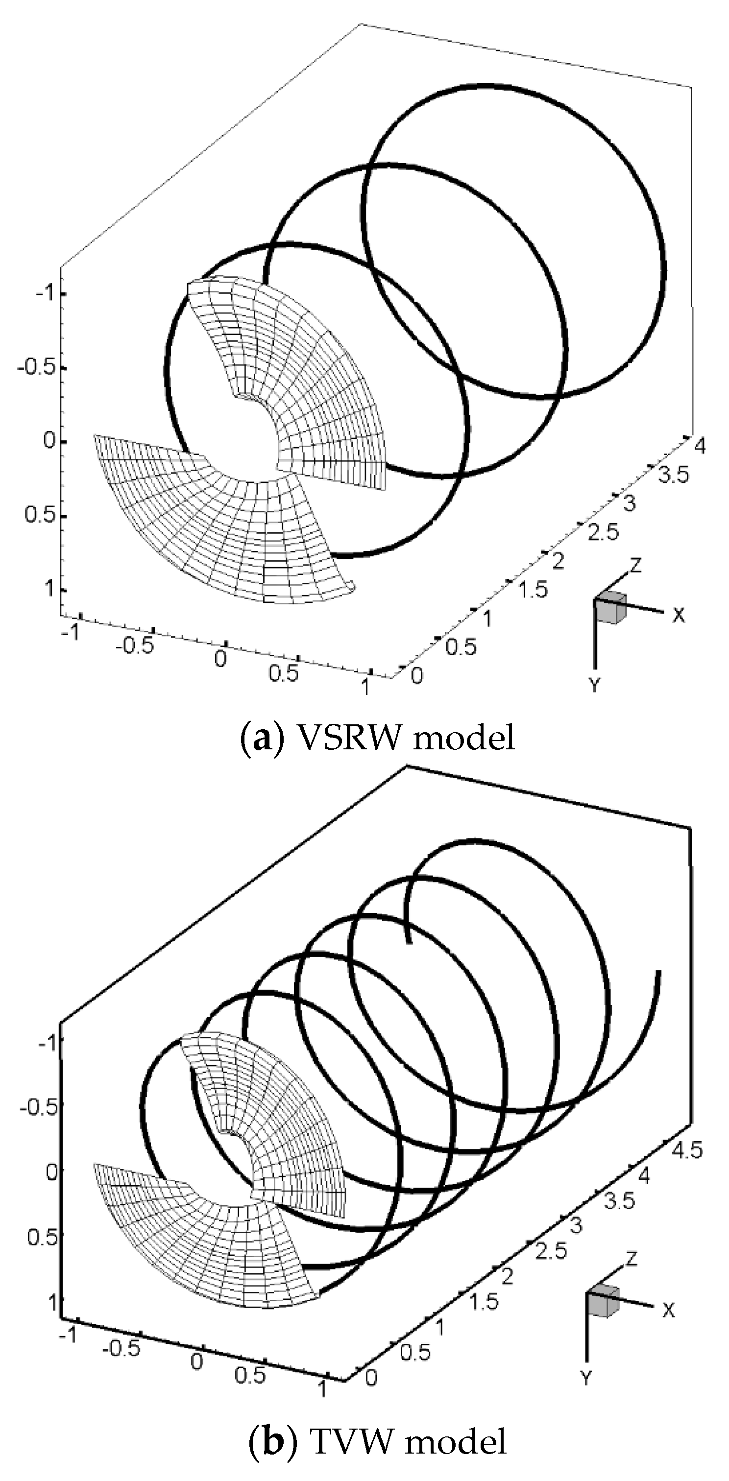
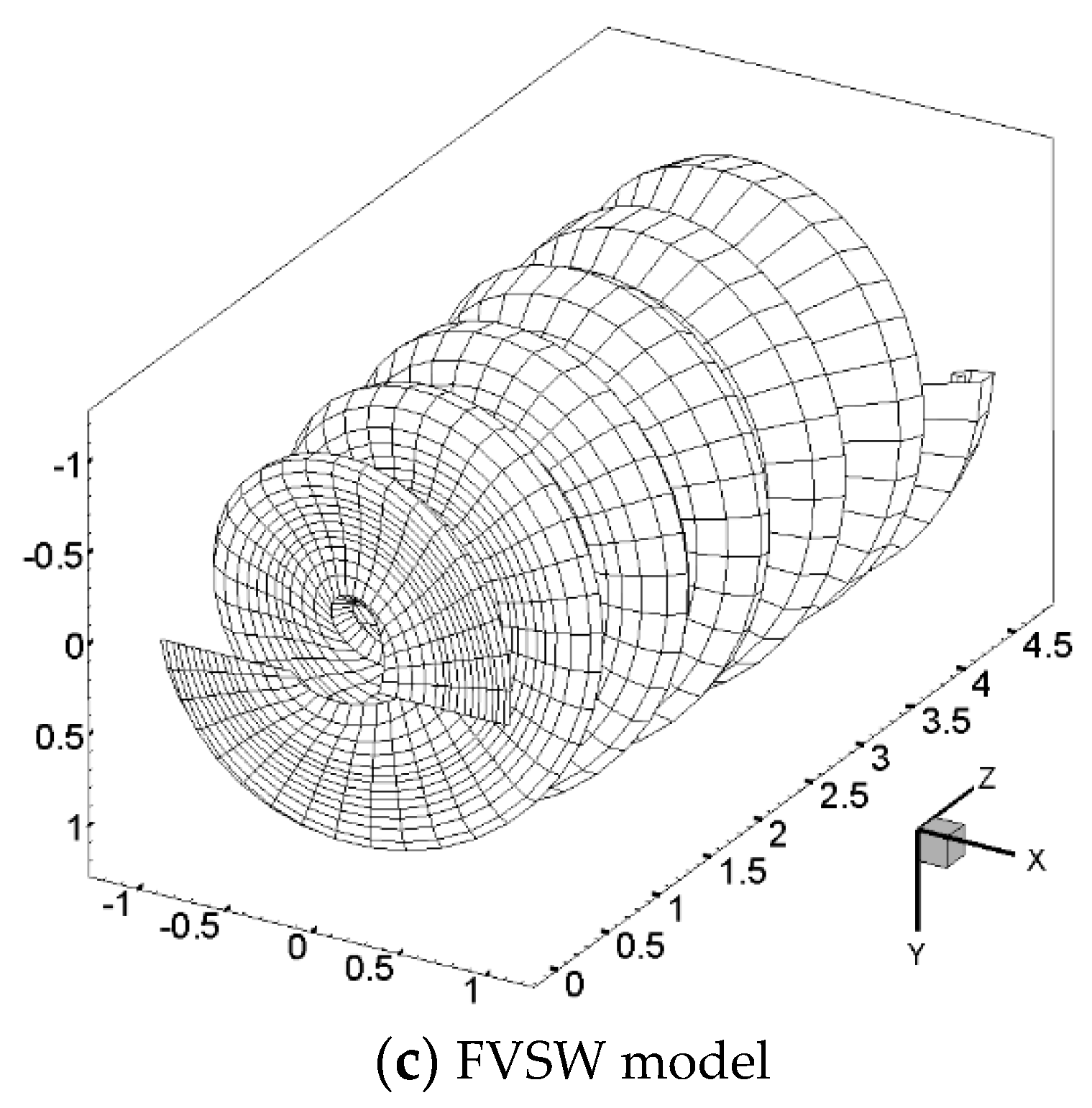
4. Description of TVW and FVSW Models

To compare the calculation time and the accuracy of the proposed VSRW model with other models, the existing and mature models TVW and FVSW are used in this study. The blade models of the TVW and FVSW models are the same as the blade model of the VSRW model. As shown in Figure 2, the wake of the TVW model consists of vortex sheets in the near wake and tip vortex filaments in the far wake; the wake of the FVSW model consists of only vortex sheets in the near wake and far wake. The wake lengths of the two models are 4R and the near wake length of the TVW model was also set at 120°. The five-point central difference approximation [21] and the pseudo-implicit technique [23,24] are used to solve the convection equation of the vortex filaments in all the wakes of the TVW and FVSW models. The prescribed tolerances of the RMS change are all set as 10−4.

5. Results and Discussions
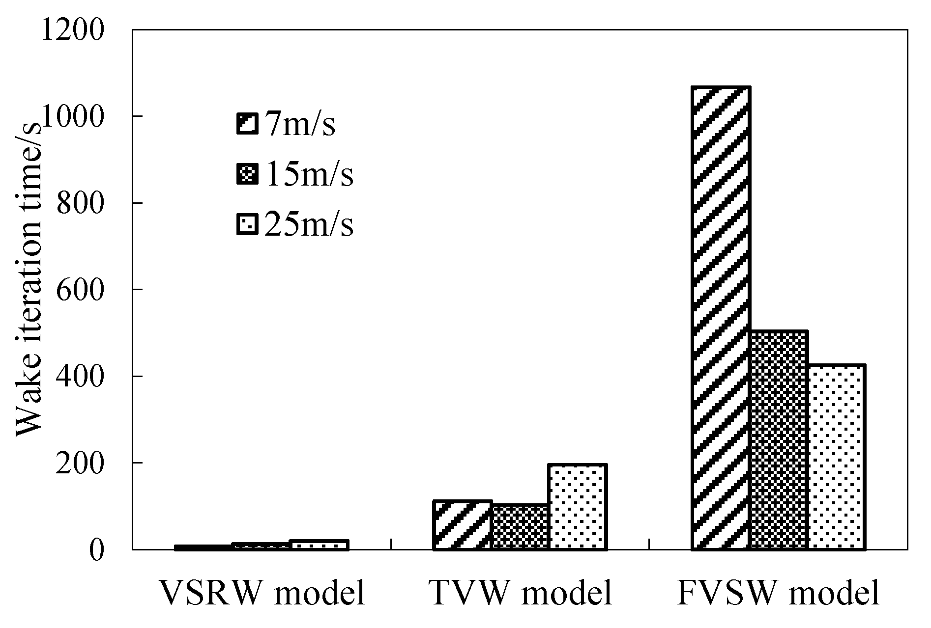
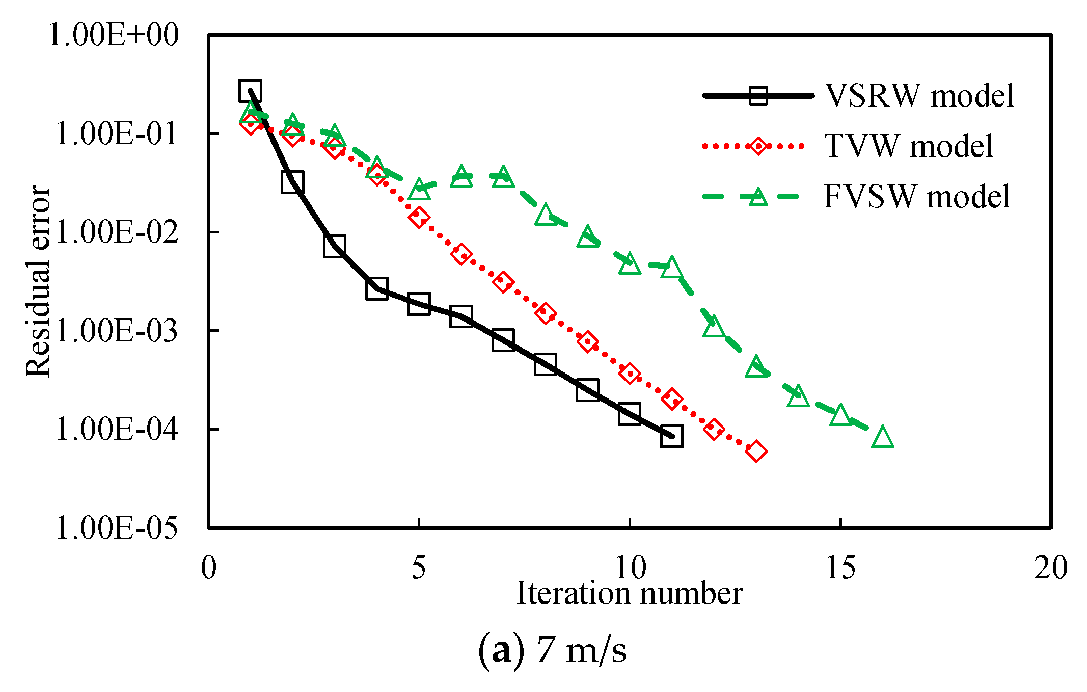
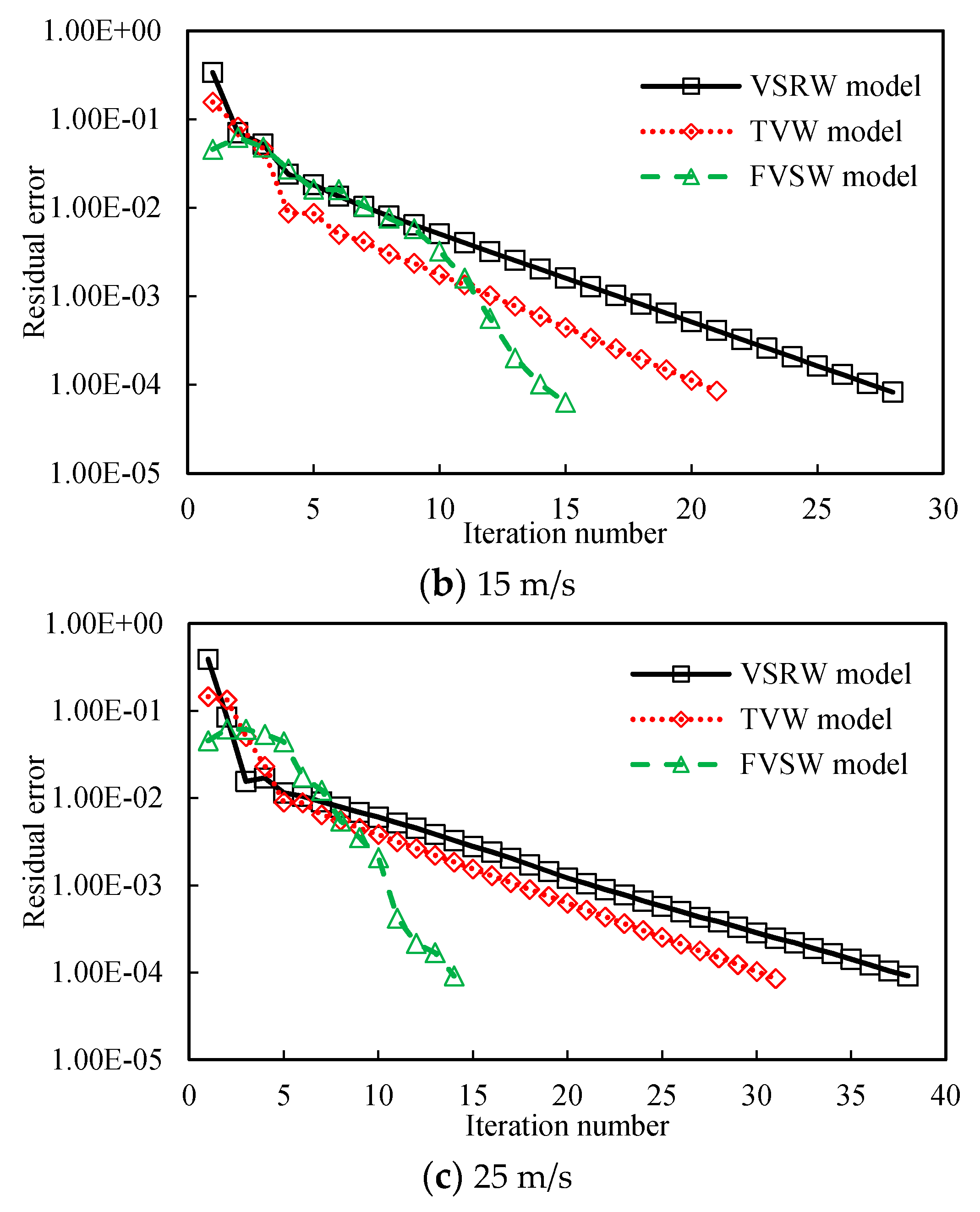
5.1. Wake Iteration

In this study, we focus on decreasing the calculation time of the vortex model, which is approximately equal to the computational cost for the wake iteration. Figure 9 shows the wake iteration time of the VSRW model, TVW model, and FVSW model at the wind speeds of 7 m/s, 15 m/s, and 25 m/s. The wake iteration of the VSRW model requires 7.94 s, 13.37 s, and 20.24 s at the three wind speeds respectively; the computation speed is far faster than the two other models. The wake iteration time of the VSRW model at 7 m/s is two orders of magnitude less than for the FVSW model and the other times are one order of magnitude less. The VSRW model can generate results much faster than the two conventional methods mainly for two following reasons.
(1)
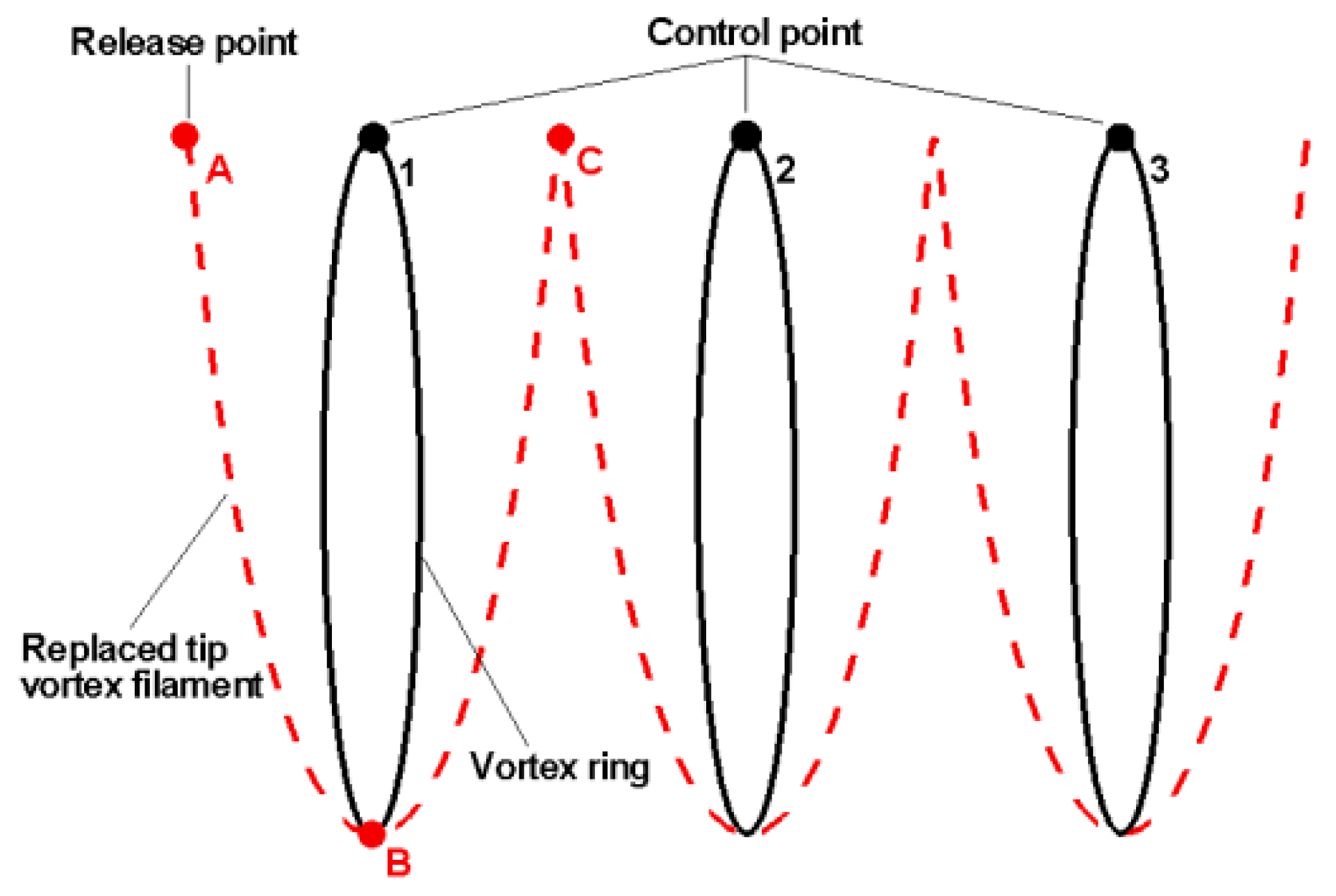
In the VSRW model, the position of the vortex ring is determined by its control point, so we just have to calculate the induced velocity and the position of the control point of the vortex ring in the far wake. However, in the conventional methods, induced velocities and positions of all nodes of the vortex filaments in the far wake need to be calculated.
(2)
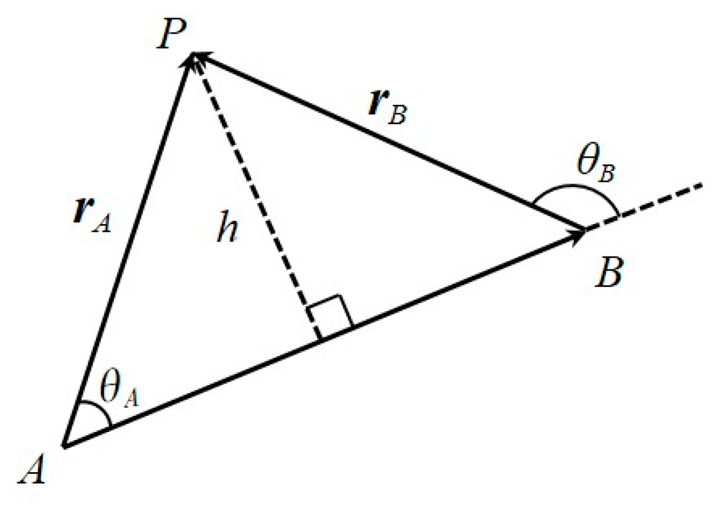
The analytical method described in Section 2.4.2 is used to calculate the velocity induced by the far wake in the VSRW model. In the conventional methods, the velocity induced by the far wake is the sum of the velocities induced by the straight-line vortex elements, which are calculated using the Biot–Savart law.
Figure 10 shows the convergence histories of the RMS of the error in the wake geometries at wind speeds of 7 m/s, 15 m/s, and 25 m/s using the three wake models. The convergence iteration numbers of the VSRW and TVW models are higher when the wind speed is higher. However, the convergence iteration number of the FVSW model does not change much with increasing wind speed. The wake iteration time depends on the convergence iteration number and the computational time of each step. In the TVW and FVSW models, more resources are needed to calculate the induced velocity field and the positions of the wake nodes; this results in a longer wake iteration time as shown in Figure 9. This is apparent in the FVSW model because of the dense vortex sheets, especially at a wind speed of 7 m/s. The introduction of the vortex ring technology in the far wake of the proposed VSRW model saves a lot of calculation time for determining the induced velocity field of the vortex rings and the positions of the vortex ring control points; as a result, the computational time for each step is greatly reduced. Therefore, the wake iteration time is still very short at a high wind speed although the convergence iteration number increases markedly.

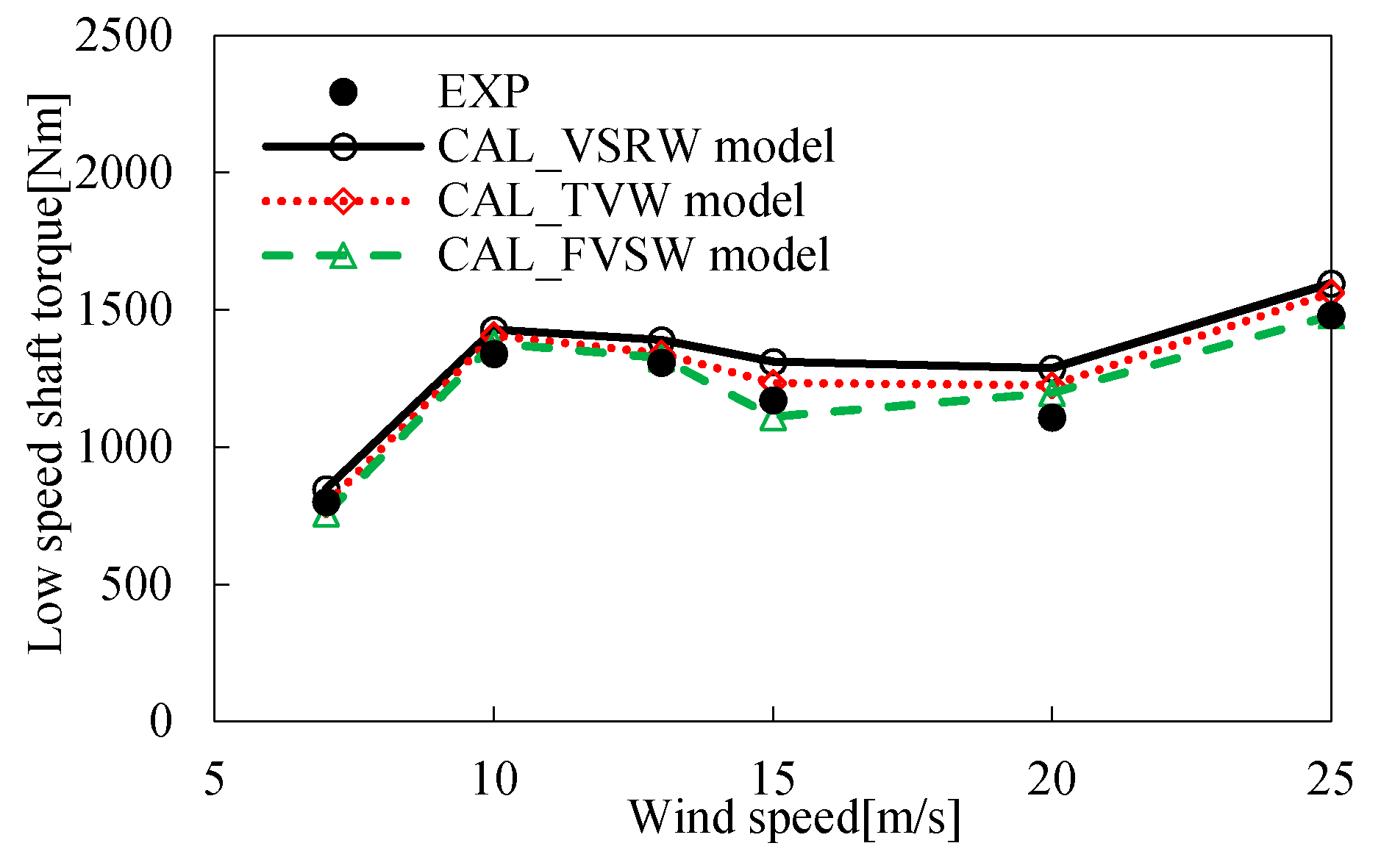
5.2. Low Speed Shaft Torque

The computational time of the proposed VSRW model can be greatly reduced and in the following section, we analyze its accuracy. The aerodynamic load of the LSST is predicted by the three different wake models. Figure 11 shows the aerodynamic estimates from the models compared with the values measured directly at the shaft [35]. The trends of the calculated results are consistent with the measurement results. Above 15 m/s, the estimated values begin to differ from each other and from the value measured at the shaft. The reason is that most of the blade is undergoing a stall flow. Although the 2D airfoil data are modified by the stall-delay model, the accurate prediction of the aerodynamic load in rotational and stall conditions is still challenging. This is also reflected in the studies by Breton et al. [37] who used a prescribed vortex wake technique and by Sant et al. [6] who used a free vortex wake technique. All the results from the VSRW model are slightly higher than those from the TVW and FVSW models. Except for 20 m/s, the results from the VSRW model could have errors no more than 10% relative to the experiment data. At 20 m/s, the error relative to the experiment data is about 16%. However, it is gratifying that the simplification of the far wake in the VSRW model did not significantly affect the accuracy of the aerodynamic load prediction.

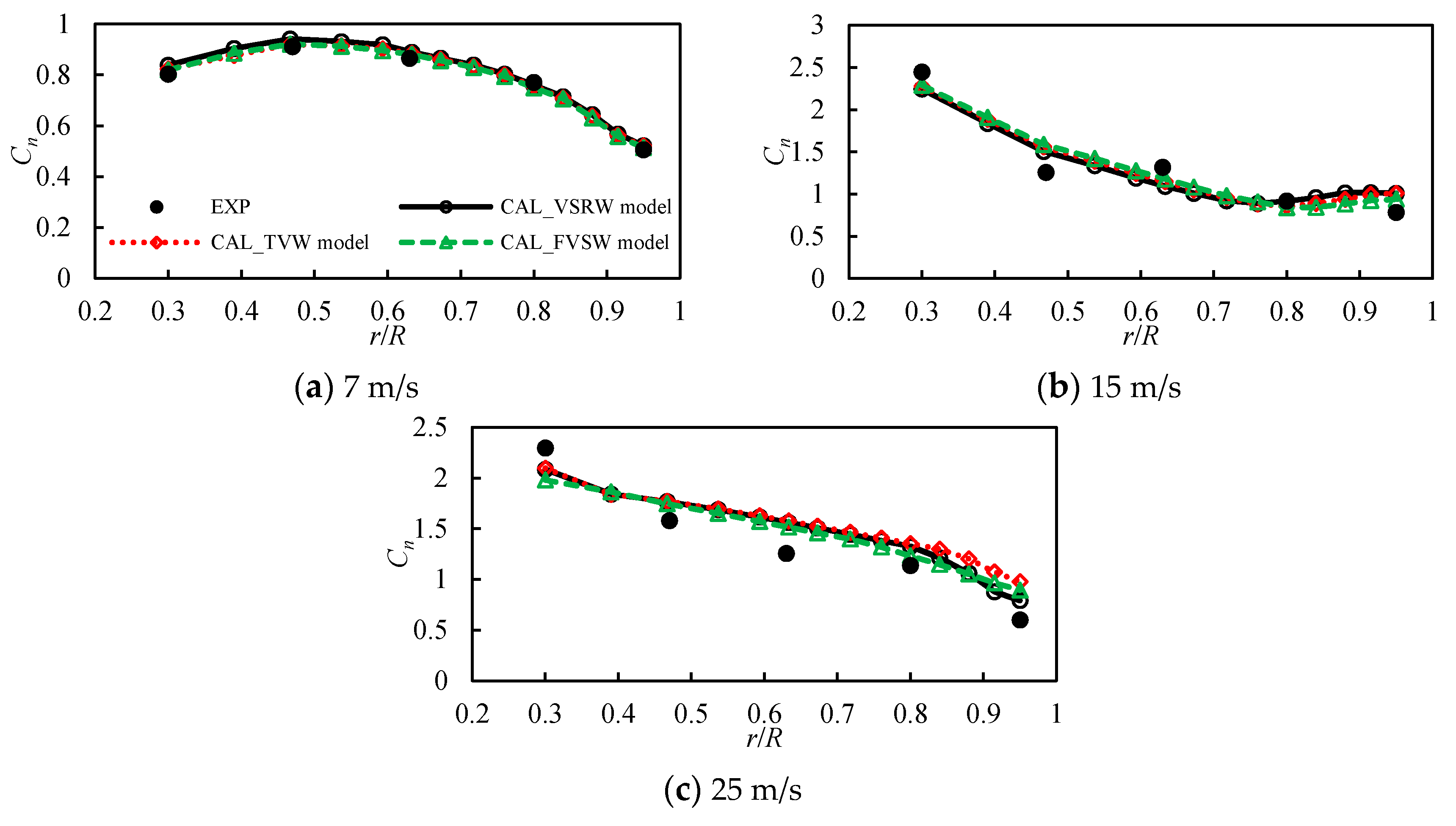
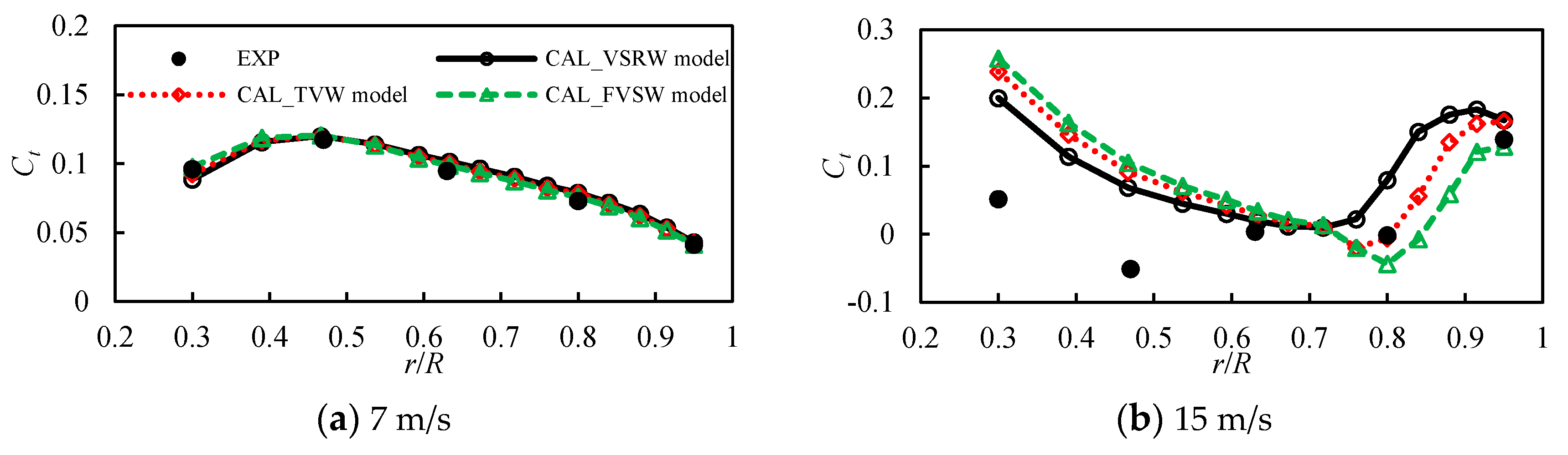
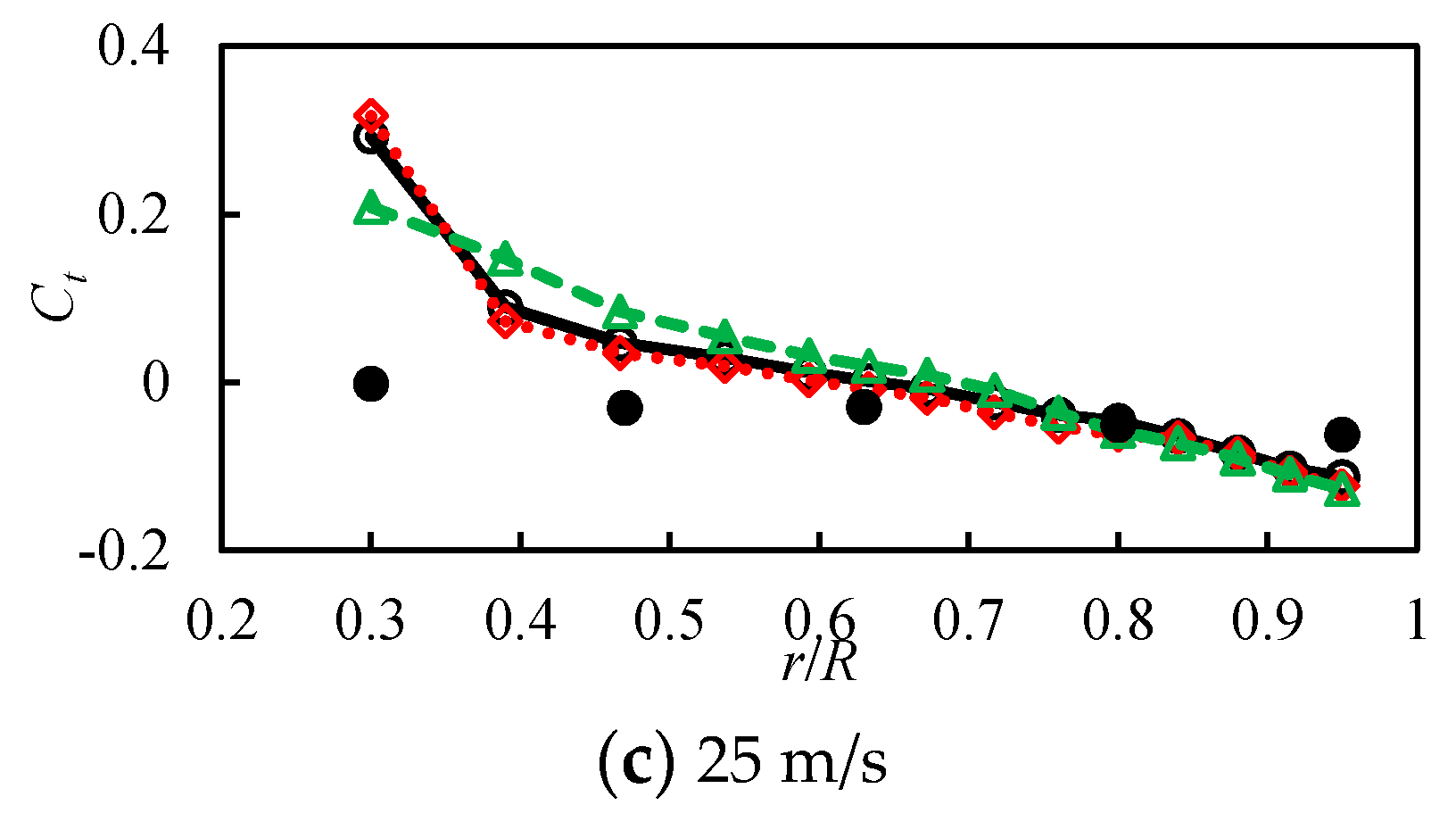
5.3. Radial Distribution of Blade Airloads

The distributions of the normal and tangential force coefficients ( C n and C t ) at different wind speeds are computed by the proposed VSRW model, the TVW model, and the FVSW model. Figure 12 and Figure 13 show the normal force coefficients and the tangential force coefficients respectively at 7 m/s, 15 m/s, and 25 m/s from the models and comparisons with the measurement results [35]. It is evident that the trends of the distributed airloads along the blade span are consistent with the measurement results. At 7 m/s, C n and C t derived by the three models agree well with the measurement results; C n and C t predicted by the VSRW model could have errors no more than 5% and 9% respectively relative to the experiment data. At high wind speeds of 15 m/s and 25 m/s, the estimated values, especially C t , begin to differ from each other and from the measurement results because most of the blade is undergoing a stall flow. The comparison results exhibit similarities to the calculation of the LSST and illustrate that the proposed VSRW model predicts the radial distribution of the blade airloads as well as the TVW and FVSW models.

5.4. Wake Geometry

Figure 14 shows the wake geometries at 10 m/s computed using the three different wake models. The azimuthal angle of the wake geometry is 0°. The wake deformation computed by using the FVSW model differs from that shown in Figure 2a. The wake deformation of the near wake of the VSRW and TVW models is also shown. The number of discrete wake nodes is far higher for the FVSW model than for the VSRW and TVW models; therefore, more computational time is required. It should be noted that the vortex rings from the two blades overlap at the same axial position. Therefore, there are actually six vortex rings in Figure 14a.

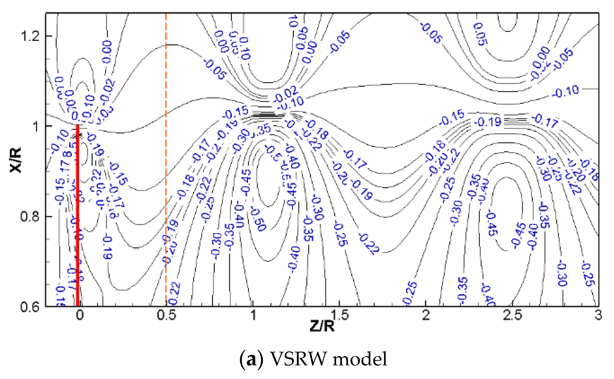
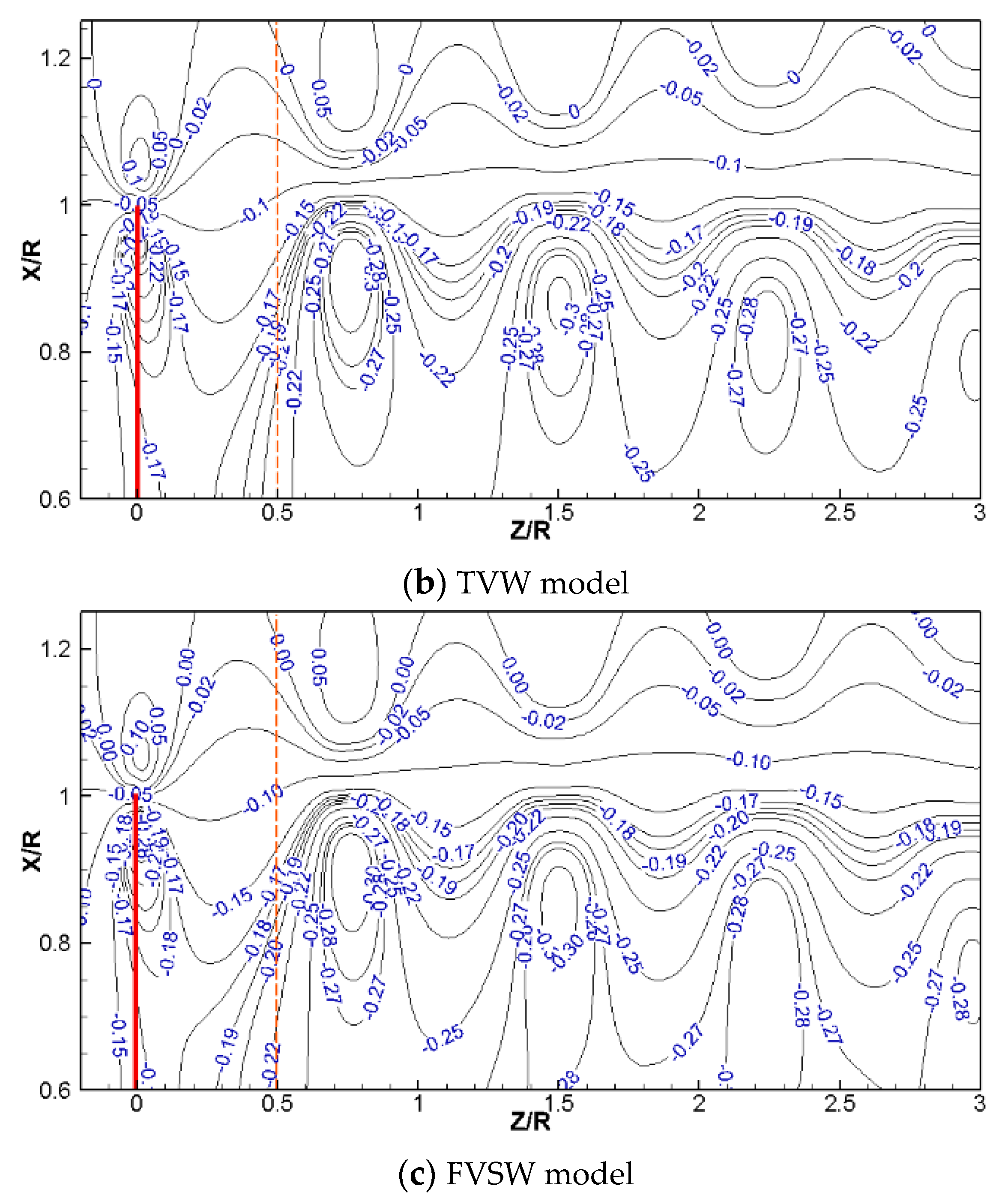
5.5. Induction Factor in the Wake

Figure 15 shows the contours of the axial induction factor in the XOZ plane at the blade azimuthal angle of 0°. In the front of the plane Z/R = 0.5 (on the left of the red dashed line in Figure 14), the distributions of the axial induction factor are similar for the three wake models. On the right of the red dashed line, the patterns of the contours of the axial induction factor are similar for the TVW and FVSW models but a marked difference is observed for the VSRW model. This is because the vortex rings are used to replace the helical tip vortex filament in the far wake. The radial expansion deformation of the wake can be captured by the VSRW model, as well as the other two models. The two overlapping vortex rings at the same axial position are the reason that the maximum axial induction factor around the vortex ring is twice as high as the maximum value in the TVW and FVSW models. On the motion trail of the tip vortex, the axial induction factor remains at about −0.1 in three wake models; therefore, the assumption of the constant induced velocity is reasonable when the control point is moving.

6. Conclusions

In this study, a simplified FVW model was developed to rapidly calculate the aerodynamic performance of wind turbines in axial steady conditions. The helical tip vortex filament of the far wake in the traditional FVW model is replaced by several vortex rings. The proposed computing method of the vortex ring position and the proposed analytical formulas of the vortex ring-induced velocity greatly reduce the computational time. The length of the near wake was cut off at a 120° wake age angle to take into account both the accuracy and the calculation time of the VSRW model. The computational speed of the simplified FVW model is at least an order of magnitude faster than other two conventional models and the convergence and stability are good.
The simplified FVW model accurately predicts the blade aerodynamic load, including the LSST and the distributions of the span’s normal and tangential force coefficients. The error of the low speed shaft torque obtained from the simplified FVW model is no more than 10% relative to the experiment at most wind speeds. The normal and tangential force coefficients obtained from the three models agree well with each other and with the measurement results at the low wind speed. At the high wind speed, the estimated values begin to differ from each other and from the measurement results because most of the blade is undergoing a stall flow
Except for differences in the axial induction factor field in the far wake, the axial induction factor field in the near wake computed by using the simplified FVW model agrees well with the other two FVW models and the radial expansion deformation of the wake is captured. The comparison of the far wake structure illustrates that the helical tip vortex filament, which is used in the TVW model, is more appropriate based on the physics of the flow.
Overall, in axial steady conditions, the computational time of the simplified FVW model is at least an order of magnitude less than that of traditional FVW models and the prediction accuracy is not affected significantly. On this basis, a study of the unsteady simplified FVW model will be conducted in the future.

Author Contributions

B.X. run the FVW codes and prepared this manuscript under the guidance of T.W. and Y.Y. Z.Z. and H.L. supervised the work and contributed in the interpretation of the results. All authors carried out data analysis, discussed the results and contributed to writing the paper.

Acknowledgments

This work was supported by the National Natural Science Foundation of China (grant number 51607058, 11502070); the National Basic Research Program of China (973 Program) (grant number 2014CB046200); and the Fundamental Research Funds for the Central Universities (grant number 2016B01514).

Conflicts of Interest

The authors declare no conflict of interest.

Nomenclature

Variables
a , b Coefficients in the induced velocity equation (-)
c i Chord of the ith blade element (m)
C l Lift coefficient (-)
C n Normal force coefficient to the rotor disc (-)
C t Tangential force coefficients to the rotor disc (-)
h Distance from the collocation point to the vortex-line segment (m)
i , k , n Integer variables (-)
N C Number of vortex rings (-)
N E Number of blade elements (-)
N T Number of time steps of a circle (-), N T = 2 π / Δ ψ
r Radial location of the blade (m)
R Rotor tip radius (m)
r ¯ b Dimensionless radial location of the blade element boundary (-)
r b Radial location of the blade element boundary (m)
r v Position vector of the vortex collocation point (m)
r A Position vector from point A to point P (m)
r B Position vector from point B to point P (m)
R c r ( n ) Radial position of the nth vortex ring control point (m)
R A Radial position of the tip vortex release (m)
R P Radial position of point P (m)
V i n d Induced velocity vector (m/s)
v i n d , r Radial velocity at point P induced by the nth vortex ring (m/s)
v i n d , z Axis velocity at point P induced by the nth vortex ring (m/s)
V i n d , R n Radial velocity at the nth vortex ring control point induced by all vortex field (m/s)
V i n d , R A Radial velocity at point A induced by all vortex field (m/s)
V i n d , Z n Axis velocity at the nth vortex ring control point induced by all vortex field (m/s)
V i n d , Z A Axis velocity at point A induced by all vortex fields (m/s)
V 0 Free stream velocity vector (m/s)
W i Resultant velocity at the control point of the ith blade element (m/s)
X X axis in the coordinate system pointing right as viewed from the front (m)
Y Y axis in the coordinate system pointing vertically downwards (m)
Z Z axis in the coordinate system in the direction of wind flow (m)
Z c r ( n ) Axis position of the nth vortex ring control point (m)
Z A Axis position of the tip vortex release (m)
Z P Axis position of point P (m)
Γ Vortex circulation (m2/s)
Γ b Bound circulation of the blade element (m2/s)
Γ n Vortex circulation of the nth vortex ring (m2/s)
Δ ζ Discretization of the azimuthal angle (rad)
Δ ψ Discretization of the wake age angle (rad)
ζ Vortex wake age angle (rad)
θ A Angle between vector r A and vector AB (rad)
θ B Angle between vector r B and vector AB (rad)
ψ Azimuthal angle (rad)
Abbreviations
BEMblade element momentum
CFDcomputational fluid dynamics
CPUCentral Processing Unit
FVSWfull vortex sheet wake
FVWfree vortex wake
GPUGraphics Processing Unit
LSSTlow speed shaft torque
NASANational Aeronautics and Space Administration
NRELNational Renewable Energy Laboratory
RMSroot mean square
TVWtip vortex wake
VSRWvortex sheet and ring wake
WInDSWake Induced Dynamics Simulator

References

  1. Hansen, M.O.L.; Sørensen, J.N.; Voutsinas, S.; Sørensen, N.; Madsen, H.A. State of the art in wind turbine aerodynamics and aeroelasticity. Aerosp. Sci. 2006, 42, 285–330. [Google Scholar] [CrossRef]
  2. Fernandez-Gamiz, U.; Zulueta, E.; Boyano, A.; Ansoategui, I.; Uriarte, I. Five megawatt wind turbine power output improvements by passive flow control devices. Energies 2017, 10, 742. [Google Scholar] [CrossRef]
  3. Gohard, J.C. Free Wake Analysis of Wind Turbine Aerodynamics, Wind Energy Conversion, ASRL-TR-184-14; Massachusetts Institute of Technology, Department of Aeronautics and Astronautics, Aeroelastic and Structures Research Laboratory: Cambridge, MA, USA, 1978. [Google Scholar]
  4. Arsuffi, G.; Guj, G.; Morino, L. Boundary element analysis of unsteady aerodynamics aerodynamics of windmill rotors in the presence of yaw. J. Wind Eng. Ind. Aerodyn. 1993, 45, 153–173. [Google Scholar] [CrossRef]
  5. Garrel, A.V. Development of a Wind Turbine Aerodynamics Simulation Module; ECN-C-03-079; Energy Research Centre of The Netherlands: Petten, The Netherlands, 2003. [Google Scholar]
  6. Sant, T.; Kuik, G.V.; Bussel, G. Estimating the Angle of Attack from Blade Pressure Measurements on the NREL Phase VI Rotor Using a Free Wake Vortex Model: Axial Conditions. Wind Energy 2006, 9, 549–577. [Google Scholar] [CrossRef]
  7. Sebastian, T.; Lackner, M.A. Development of a free vortex wake method code for offshore floating wind turbines. Renew. Energy 2012, 46, 269–275. [Google Scholar] [CrossRef]
  8. Rosen, A.; Lavie, I.; Seginer, A. A general free-wake efficient analysis of horizontal-axis wind turbines. Wind Eng. 1990, 14, 362–373. [Google Scholar]
  9. Gupta, S. Development of a Time-Accurate Viscous Lagrangian Vortex Wake Model for Wind Turbine Applications. Ph.D. Dissertation, University of Maryland, College Park, MD, USA, 2006. [Google Scholar]
  10. Qiu, Y.X.; Wang, X.D.; Kang, S.; Zhao, M.; Liang, J.Y. Predictions of unsteady HAWT aerodynamics in yawing and pitching using the free vortex method. Renew. Energy 2014, 70, 93–105. [Google Scholar] [CrossRef]
  11. Xu, B.F.; Wang, T.G.; Yuan, Y.; Cao, J.F. Unsteady aerodynamic analysis for offshore floating wind turbines under different wind conditions. Philos. Trans. R. Soc. A 2015, 373, 20140080. [Google Scholar] [CrossRef] [PubMed]
  12. Marten, D.; Lennie, M.; Pechlivanoglou, G.; Nayeri, C.N.; Paschereit, C.O. Implementation, optimization and validation of a nonlinear lifting line free vortex wake module within the wind turbine simulation. In Proceedings of the ASME Turbo Expo 2015: Turbine Technical Conference and Exposition, Montreal, QC, Canada, 15–19 June 2015. [Google Scholar]
  13. Miller, R.H. The aerodynamics and dynamic analysis of horizontal axis wind turbines. J. Wind Eng. Ind. Aerodyn. 1983, 15, 329–340. [Google Scholar] [CrossRef]
  14. Afjeh, A.A.; Keith, T.G.J. A vortex lifting line method for the analysis of horizontal axis wind turbines. ASME J. Sol. Energy Eng. 1986, 108, 303–309. [Google Scholar] [CrossRef]
  15. Yu, W.; Ferreira, C.S.; van Kuik, G.; Baldacchino, D. Verifying the blade element momentum method in unsteady, radially varied, axisymmetric loading using a vortex ring model. Wind Energy 2017, 20, 269–288. [Google Scholar] [CrossRef]
  16. Farrugia, R.; Sant, T.; Micallef, D. Investigating the aerodynamic performance of a model offshore floating wind turbine. Renew. Energy 2014, 70, 24–30. [Google Scholar] [CrossRef]
  17. Elgammi, M.; Sant, T. Combining unsteady blade pressure measurements and a free-wake vortex model to investigate the cycle-to-cycle variations in wind turbine aerodynamic blade loads in yaw. Energies 2016, 9, 460. [Google Scholar] [CrossRef]
  18. Turkal, M.; Novikov, Y.; Usenmez, S.; Sezer-Uzol, N.; Uzol, O. GPU based fast free-wake calculations for multiple horizontal zxis wind turbine rotors. J. Phys. Conf. Ser. 2014, 524, 012100. [Google Scholar] [CrossRef]
  19. Weissinger, J. The Lift Distribution of Swept-Back Wings; NACA-TM-1120; National Advisory Committee for Aeronautics: Cleveland, OH, USA, 1947. [Google Scholar]
  20. Du, Z.; Selig, M.S. A 3-D Stall-Delay Model for Horizontal Axis Wind Turbine Performance Prediction; AIAA-98–0021; American Institute of Aeronautics and Astronautics: Reston, VA, USA, 1998. [Google Scholar]
  21. Bagai, A.; Leishman, J.G. Rotor free-wake modeling using a relaxation technique—Including comparisons with experimental data. J. Am. Helicopter Soc. 1995, 40, 29–41. [Google Scholar] [CrossRef]
  22. Bhagwat, M.; Leishman, J.G. Stability, consistency and convergence of time marching free-vortex rotor wake algorithms. J. Am. Helicopter Soc. 2001, 46, 59–71. [Google Scholar] [CrossRef]
  23. Grouse, G.L.; Leishman, J.G. A new method for improved rotor free vortex convergence. In Proceedings of the 31st AIAA Aerospace Sciences Meeting and Exhibit, Reno, NV, USA, 11–14 January 1993. [Google Scholar]
  24. Wang, T.G.; Wang, L.; Zhong, W.; Xu, B.F.; Chen, L. Large-scale wind turbine blade design and aerodynamic analysis. Chin. Sci. Bull. 2012, 57, 466–472. [Google Scholar] [CrossRef]
  25. Gupta, S.; Leishman, J.G. Accuracy of the induced velocity from helicoidal vortices using straight-line segmentation. AIAA J. 2005, 43, 29–40. [Google Scholar] [CrossRef]
  26. Vatistas, G.H.; Kozel, V.; Minh, W. A simpler model for concentrated vortices. Exp. Fluids 1991, 11, 73–76. [Google Scholar] [CrossRef]
  27. Sant, T.; del Campo, V.; Micallef, D.; Ferreira, C.S. Evaluation of the lifting line vortex model approximation for estimating the local blade flow fields in horizontal-axis wind turbines. J. Renew. Sustain. Energy 2016, 8, 023302. [Google Scholar] [CrossRef] [Green Version]
  28. Gupta, S.; Leishman, J.G. Validation of a free vortex wake model for wind turbine in yawed flow. In Proceedings of the 44th AIAA Aerospace Sciences Meeting 2006, Reno, NV, USA, 9–12 January 2006; Volume 7, pp. 4529–4543. [Google Scholar]
  29. Xu, B.F.; Yuan, Y.; Wang, T.G.; Zhao, Z.Z. Comparison of two vortex models of wind turbines using a free vortex wake scheme. J. Phys. Conf. Ser. 2016, 753, 022059. [Google Scholar] [CrossRef]
  30. Xu, B.F.; Feng, J.H.; Wang, T.G.; Yuan, Y.; Zhao, Z. Application of a turbulent vortex core model in the free vortex wake scheme to predict wind turbine aerodynamics. J. Renew. Sustain. Energy 2018, 10, 023303. [Google Scholar] [CrossRef]
  31. Bhagwat, M.J.; Leishman, J.G. Correlation of helicopter tip vortex measurements. AIAA J. 2000, 38, 301–308. [Google Scholar] [CrossRef]
  32. Ananthan, S.; Leishman, J.G. The role of filament stretching in the free-vortex modeling of rotor wakes. J. Am. Helicopter Soc. 2004, 49, 176–191. [Google Scholar] [CrossRef]
  33. Yoon, S.S. Heister, S.D. Analytical formulas for the velocity field induced by an infinitely thin vortex ring. Int. J. Numer. Methods Fluids 2004, 44, 665–672. [Google Scholar] [CrossRef]
  34. Fukushima, T. Fast computation of complete elliptic integrals and Jacobian elliptic functions. Celest. Mech. Dyn. Astron. 2009, 105, 305–328. [Google Scholar] [CrossRef]
  35. Hand, M.M.; Simms, D.A.; Fingersh, L.J.; Jager, D.W.; Cotrell, J.R.; Schreck, S.; Larwood, S.M. Unsteady Aerodynamics Experiment Phase VI: Wind Tunnel Test Configurations and Available Data Campaign; NREL/TP-500-29955; National Renewable Energy Laboratory: Golden, CO, USA, 2001.
  36. Ananthan, S. Analysis of Rotor Wake Aerodynamics during Maneuvering Flight Using a Free-Vortex Wake Methodology. Ph.D. Dissertation, University of Maryland, College Park, MD, USA, 2006. [Google Scholar]
  37. Breton, S.P.; Coton, F.N.; Moe, G. A study on rotational effects and different stall delay models using a prescribed wake vortex scheme and NREL Phase VI experiment data. Wind Energy 2008, 11, 459–482. [Google Scholar] [CrossRef]
Figure 1. Schematic of the initial wakes of different FVW models. (a) FVSW model. (b) TVW model.
Applsci 08 00866 g001
Figure 2. Schematic of the blade model and the vortex wake model.
Applsci 08 00866 g002
Figure 3. Schematic of the far wake.
Applsci 08 00866 g003
Figure 4. Schematic of the straight-line vortex elements.
Applsci 08 00866 g004
Figure 5. Schematic of the coordinate system for the induced velocity calculation of the vortex ring.
Applsci 08 00866 g005
Figure 6. Flowchart of the simplified FVW model.
Applsci 08 00866 g006
Figure 7. LSST along the length of the near wake at different wind speeds (The red points are the LSST values with a near wake age angle of 120°).
Applsci 08 00866 g007
Figure 8. Wake iteration time along the length of the near wake at 7 m/s and 15 m/s.
Applsci 08 00866 g008
Figure 9. Wake iteration time of the VSRW model, TVW model, and FVSW model at 7 m/s, 15 m/s, and 25 m/s.
Applsci 08 00866 g009
Figure 10. Convergence history of the RMS of the error in the wake geometry.
Applsci 08 00866 g010aApplsci 08 00866 g010b
Figure 11. Measured and calculated results of LSST of NREL Phase VI wind turbine for wind speeds ranging from 7 m/s to 25 m/s.
Applsci 08 00866 g011
Figure 12. Comparison of the distributions of the computed normal force coefficients at (a) 7 m/s, (b) 15 m/s, and (c) 25 m/s along the blade radial positions for NREL Phase VI in axial steady conditions.
Applsci 08 00866 g012
Figure 13. Comparison of the distributions of the computed tangential force coefficients at (a) 7 m/s, (b) 15 m/s, and (c) 25 m/s along the blade radial positions for NREL Phase VI in axial steady conditions.
Applsci 08 00866 g013aApplsci 08 00866 g013b
Figure 14. Wake geometries (front view) at four times the radius distance behind the rotor at 10 m/s calculated using the (a) VSRW model, (b) TVW model, and (c) FVSW model.
Applsci 08 00866 g014aApplsci 08 00866 g014b
Figure 15. Contours of the axial induction factor.
Applsci 08 00866 g015aApplsci 08 00866 g015b

