Stability Analysis of Mixed Convection Flow towards a Moving Thin Needle in Nanofluid

Abstract

The problem of steady laminar mixed convection flow and heat transfer past a moving vertical thin needle in nanofluid for both assisting and opposing cases is analyzed in this paper. Three types of nanoparticles including copper, titania and alumina are taken into consideration. The nonlinear ordinary differential equations for momentum and energy have been transformed by adopting the similarity transformation in linear form. The problem is solved numerically using an implemented package called bvp4c in MATLAB software. The numerical computations are carried out for various parameters of interest, which consists of the velocity ratio parameter, mixed convection parameter, nanoparticle volume fraction parameter and the needle size. A stability analysis of the solution is performed showing that the upper branch solution is stable, while the lower branch solution is unstable. Validation of the present work is done by comparing the current results with those available in the existing literature and found to be in excellent agreement.

1. Introduction

Along with the development of technology, most engineers have ventured to create a new system of application. Previously, most of the systems used in industries considered the conventional heat transfer fluid such as oil, water and ethylene glycol. Unfortunately, these types of heat transfer fluids did not show good performance in a cooling system. Choi [1] found an alternative way to overcome this disadvantage by introducing the term nanofluid in fluid dynamics. The usage of the nanofluid as a cooling device will intrinsically enhance the thermal performance of the manufacturing processes and also reduce the operating costs. In fact, nanofluid is formed by adding some of the nanometer-sized particles (called nanoparticles), the diameter of which is less than 100 nm, into the base fluid. There are a few types of nanoparticles such as metal, oxide, carbides and carbon nanotubes. Nanofluid possesses some special behaviors, by which it is very stable and does not have any additional problems such as erosion, sedimentation, non-Newtonian behavior or additional pressure drop. This happens due to the tiny size of the nano-elements and low volume fraction of nano-elements needed for the thermal conductivity improvement. In view of its applications, nanofluid has the potential of being a new generation of coolants in automotive applications. It tends to cool down in the electronic application effectively by removing the high heat flux such as liquid cooling, air cooling and two-phase cooling. It is also helpful in cancer imaging and drug delivery for cancer therapeutics in biomedical industries [2,3,4].

The comprehensive literature on the mathematical models of nanofluid is reported by some researchers such as Khanafer et al. [5], Buongiorno [6], Tiwari and Das [7], Nield and Kuznetsov [8], as well as Kuznetsov [9]. The effectiveness of the thermal conductivity of nanofluid among the models is studied in order to compare the theoretical data with the experimental data. There are two common types of nanofluid models that have been considered in fluid dynamics, namely the model proposed by Buongiorno [6] and Tiwari and Das [7]. Buongiorno’s model is a two-phase model in which the slip velocity between base fluid and nanoparticles is not equal to zero. This model takes into account seven slip mechanisms, which produce a relative velocity between the base fluid and nanoparticles such as inertia, thermophoresis, diffusiophoresis, Brownian motion, fluid drainage, gravity and the Magnus effect. In contrast with Buongiorno’s model, the Tiwari and Das model is a single-phase model that considers the viscosity model proposed by Brinkman [10]. Since this model is a phase model, base fluid and nanoparticles are said to be in thermal equilibrium, flowing at a uniform velocity, and a no-slip condition occurs between them. This model considers the effect of nanoparticles volume fraction. There are several articles regarding these two models that can be found in the literature [11,12,13,14].

Due to the importance of several industrial and technological applications, researchers are now grabbing the opportunity to investigate the boundary layer flow and heat transfer analysis induced by a thin needle in various fluid. The term thin needle simply means a parabolic revolution about its axes direction in addition to the variable thickness. The motion of the thin needle distracts from the free stream direction, and this situation is the main concern in experimental studies for the flow and heat transfer analysis in order to measure the velocity and temperature profiles of the system. It has many practical applications especially in the medicine and engineering industries. Some of the applications are a hot wire anemometer for measuring the velocity of the wind, the blood flow problem, transportation, coating of wires, lubrication and geothermal power generation.

The boundary layer flow past a thin needle in viscous fluid have been studied by Lee [15]. According to Lee [15], a needle is assumed “thin” when its thickness is smaller than or comparable to that of the boundary layer over it. Inspired by the work of Lee [15], Narain and Uberoi [16] and Narain and Uberoi [17] further investigate the problem by considering the mixed convection flow over a vertical thin needle in viscous fluid. Since then, numerous works regarding the boundary layer flow over a thin needle were carried out [18,19,20,21]. However, the previously-mentioned works deals only with viscous fluid. Following from there, Grosan and Pop [22] grabbed the opportunity to study the boundary layer flow of a horizontal thin needle in nanofluid. In their work, they solved the classical problem of forced convection flow and heat transfer with a variable wall temperature. Starting from that, many investigations into nanofluid were carried out by Hayat et al. [23], Soid et al. [24], Krishna et al. [25] and Ahmad et al. [26] for various aspects of the problem. In contrast to the problem of the horizontal thin needle, the consideration of studying the vertical thin needle is less popular and was carried out by Trimbitas et al. [27]. In their study, they consider the mixed convection boundary layer flow in nanofluid past a stationary vertical thin needle with the presence of gravitational force.

The study of the stationary needle has substantially different types of solutions from the moving needle. This is due to the entrapment of the ambient temperature for the moving surface, which causes the flow situation to represent an essentially different class of boundary layer flows. There are some practical applications that prove the boundary layer behavior on the moving surface is an imperative aspect of flow appearing in industrial and engineering processes. Some applications include the boundary layer past a liquid film in condensation processes, aerodynamic extrusion of a plastic sheet and a long thread traveling between a feed roll and a wind-up roll [28,29]. Since numerous applications have been found in industries involving the moving surface, the purpose of this paper is to investigate the characteristics of the fluid flow and heat transfer analysis past a moving vertical thin needle in nanofluid under the influence of gravity (body) forces using the Tiwari and Das model. This problem considers both assisting and opposing flow. The partial differential equations for momentum and energy are reduced to ordinary differential equations, which are then solved numerically using an implemented package bvp4c in MATLAB software (Matlab R2013a, Mathwork, Natick, MA, USA, 1984). The side effect of the mixed convection parameter including the velocity ratio parameter, nanoparticle volume fraction parameter and the needle size are graphically presented and elaborated in detail in the next section for $Pr=6.2$ (water).

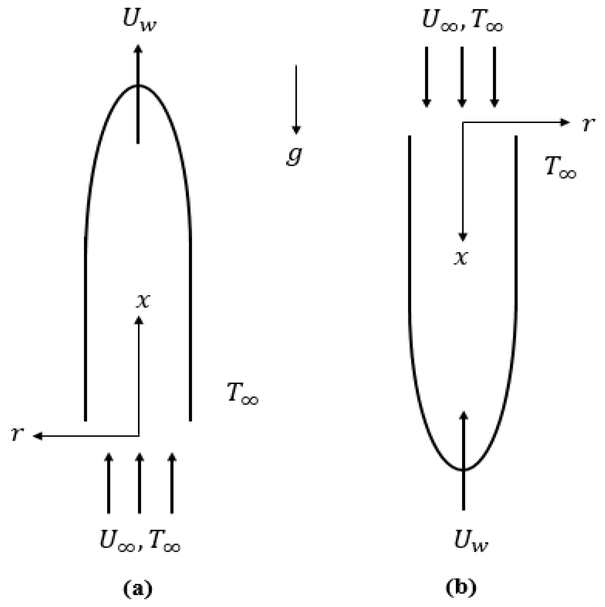
2. Problem Formulation

2.1. Basic Equation

An incompressible laminar boundary layer flow and heat transfer of a nanofluid passing through a moving vertical thin needle of uniform ambient temperature $T_{\infty }$ is considered. The inset of Figure 1 illustrates the vertical slender paraboloid needle whose radius is given by $r=R\left(x\right)$ where x and r are the axial and radial coordinates, respectively. The x-axis measures the needle’s leading edge in the vertical direction, whereas r is always normal to the x-axis. The needle is considered thin when its thickness does not exceed that of the boundary layer over it. Since the needle is assumed thin, the influence of its transverse curvature is important; however, the pressure gradient along the surface due to the presence of the needle can be ignored [15]. Furthermore, the needle is subjected to a variable surface temperature $T_w$ where $T_w>T_{\infty }$ corresponds to an assisting flow (heated surface) and $T_w<T_{\infty }$ corresponds to an opposing flow (cooled surface). The needle moves with a uniform velocity, $U_w$, in the same or reverse direction to the fluid flow of uniform velocity, $U_{\infty }$. Based on the above assumptions, the governing equations for the nanofluid model proposed by Tiwari and Das [7] take the following form of cylindrical coordinates:

$$\frac{\partial }{\partial x}\left(ru\right)+\frac{\partial }{\partial r}\left(rv\right)=0,$$

(1)

$$\frac{\partial u}{\partial t}+u\frac{\partial u}{\partial x}+v\frac{\partial u}{\partial r}=\frac{{\mu }_{nf}}{{\rho }_{nf}}\frac{1}{r}\frac{\partial }{\partial r}\left(r\frac{\partial u}{\partial r}\right)+\frac{{\left(\rho \beta \right)}_{nf}}{{\rho }_{nf}}g(T-T_{\infty }),$$

(2)

$$\frac{\partial T}{\partial t}+u\frac{\partial T}{\partial x}+v\frac{\partial T}{\partial r}=\frac{{\alpha }_{nf}}{r}\frac{\partial }{\partial r}\left(r\frac{\partial T}{\partial r}\right)$$

(3)

Assume the initial and boundary conditions of Equations (1)–(3) are:

$$t<0:u=v=0,T=T_{\infty }foranyx,r,$$

$$t\ge 0:u=U_w,v=0,T=T_{w}atr=R\left(x\right),$$

$$u\to U_{\infty },T\to T_{\infty }asr\to \infty ,$$

(4)

where u and r are the velocity components along the x and r axis, respectively, and T is the temperature of the nanofluid on the boundary layer. $\mu$ represents the viscosity; $\rho$ is the density; $\alpha$ is the thermal diffusivity; and $\beta$ is the thermal expansion coefficient in which the subscripts ‘$nf$’, ‘f’ and ‘s’ represent ‘nanofluid ’, ‘fluid’ and ‘solid’, respectively. The relation between these parameters is given by [30]:

$${\rho }_{nf}=\left(1-\varphi \right){\rho }_f+\varphi {\rho }_s,{\left(\rho C_p\right)}_{nf}=\left(1-\varphi \right){\left(\rho C_p\right)}_f+\varphi {\left(\rho C_p\right)}_s,{\left(\rho \beta \right)}_{nf}=\left(1-\varphi \right){\left(\rho \beta \right)}_f+\varphi {\left(\rho \beta \right)}_s,$$

$${\mu }_{nf}=\frac{{\mu }_f}{{(1-\varphi )}^{2.5}},{\alpha }_{nf}=\frac{k_{nf}}{{\left(\rho C_p\right)}_{nf}},\frac{k_{nf}}{k_f}=\frac{(k_s+2k_f)-2\varphi (k_f-k_s)}{(k_s+2k_f)+\varphi (k_f-k_s)}$$

(5)

Here, k and $\left(\rho C_p\right)$ represent the thermal conductivity and heat capacity, respectively. In addition, $\varphi$ represents the nanoparticle volume fraction for the nanofluid.

2.2. Steady-State Solution

In steady-state solutions, we assume $\partial /\partial t=0$. Hence, to compute the basic Equations (1)–(3) under the boundary restrictions (4), we introduce the relevant similarity transformations as follows:

$$\psi =\nu xf\left(\eta \right),\eta =\frac{U{r}^2}{\nu x},\theta \left(\eta \right)=\frac{T-T_{\infty }}{T_w-T_{\infty }}$$

(6)

Here, $\psi$ is defined as a stream function that satisfies Equation (1), and the velocity components are defined as $u=r^{-1}\partial \psi /\partial r$ and $v=-r^{-1}\partial \psi /\partial x$, respectively. Assuming $\eta =c$ (refer to the wall of the needle), Equation (6) prescribes the size and shape of the needle where its surface is given by:

$$R\left(x\right)={\left(\frac{\nu cx}{U}\right)}^{1/2}$$

(7)

Substituting Equations (5) and (6) into basic Equations (2)–(4) reduces this to the following nonlinear ordinary differential equations given by:

$$\frac{2{\left(\eta f^{″}\right)}^{\prime }}{{\left(1-\varphi \right)}^{2.5}\left[\left(1-\varphi \right)+\varphi \left({\rho }_s/{\rho }_f\right)\right]}+f{f}^{″}+\frac{(1-\varphi )+\varphi {\left(\rho \beta \right)}_s/{\left(\rho \beta \right)}_f}{(1-\varphi )+\varphi ({\rho }_s/{\rho }_f)}\frac{\lambda \theta }{4}=0,$$

(8)

$$\frac{2{\left(\eta {\theta }^{\prime }\right)}^{\prime }}{\left(1-\varphi \right)+\varphi {\left(\rho C_p\right)}_s/{\left(\rho C_p\right)}_f}\frac{k_{nf}/k_f}{Pr}+f{\theta }^{\prime }=0,$$

(9)

where prime represents the differentiation with respect to $\eta$ (similarity variable). The appropriate boundary conditions are then given by:

$$f\left(c\right)=\frac{\epsilon }{2}c,f^{\prime }\left(c\right)=\frac{\epsilon }{2},\theta \left(c\right)=1,$$

$$f^{\prime }\left(\eta \right)\to \frac{1}{2}(1-\epsilon ),\theta \left(\eta \right)\to 0as\eta \to \infty ,$$

(10)

where $\lambda$ is the mixed convection parameter, which can be expressed as:

$$\lambda =\frac{g{\beta }_f(T_w-T_{\infty })x}{U^2}=\frac{G{r}_x}{R{e}_x^2}$$

(11)

Here, $G{r}_x=g{\beta }_f(T_w-T_{\infty })x^3/{\nu }^2$ is the local Grashof number, and $R{e}_x=Ux/\nu$ is the local Reynolds number. It is worth mentioning that $\lambda >0$ represents the assisting flow, while $\lambda <0$ represents the opposing flow. $Pr=\nu /\alpha$ is the Prandtl number, and $\epsilon$ is the velocity ratio parameter between the needle and the free stream with $U=U_w+U_{\infty }$.

The skin friction coefficients, $C_f$, and the local Nusselt number, $N{u}_x$, are given by the following equations:

$$C_f={\mu }_{nf}{(\partial u/\partial r)}_{r=c}/{\rho }_f{U}^2=\frac{4}{{(1-\phi )}^{2.5}}R{e}_x^{-1/2}{c}^{1/2}{f}^{″}\left(c\right),$$

(12)

$$N{u}_x=-x{k}_{nf}{(\partial T/\partial r)}_{r=c}/k_f(T_w-T_{\infty })=-2\frac{k_{nf}}{k_f}R{e}_x^{1/2}{c}^{1/2}{\theta }^{\prime }\left(c\right),$$

(13)

2.3. Stability Analysis

It has been discovered in Weidman et al. [31] that the lower branch solutions for the forced convection flow passing through a permeable flat plate are unstable and not physically realizable. Meanwhile, the upper branch solutions are stable and physically realizable. To test these features, we need to consider the unsteady Equations (2) and (3) by introducing the new dimensionless time variable, $\tau =2Ut/x$. Note that $\tau$ is associated with an initial value problem that is consistent with the solution that will be obtained in practice (physically realizable).

From Equation (6), the new similarity solutions in terms of $\eta$ and $\tau$ are:

$$\psi =\nu xf(\eta ,\tau ),\eta =\frac{U{r}^2}{\nu x},\theta (\eta ,\tau )=\frac{T-T_{\infty }}{T_w-T_{\infty }},\tau =\frac{2Ut}{x}$$

(14)

Substituting Equation (14) into Equations (2) and (3) yields:

$$\begin{array}{c}{\displaystyle \frac{2}{{\left(1-\varphi \right)}^{2.5}\left[\left(1-\varphi \right)+\varphi \left({\rho }_s/{\rho }_f\right)\right]}}{\left(\eta {\displaystyle \frac{{\partial }^{2}f}{\partial {\eta }^2}}\right)}^{\prime }+f{\displaystyle \frac{{\partial }^{2}f}{\partial {\eta }^2}}+{\displaystyle \frac{(1-\varphi )+\varphi {\left(\rho \beta \right)}_s/{\left(\rho \beta \right)}_f}{(1-\varphi )+\varphi ({\rho }_s/{\rho }_f)}}{\displaystyle \frac{\lambda \theta }{4}}-{\displaystyle \frac{{\partial }^{2}f}{\partial \eta \partial \tau }}\\ +\tau {\displaystyle \frac{\partial f}{\partial \eta }}{\displaystyle \frac{{\partial }^{2}f}{\partial \eta \partial \tau }}=0,\end{array}$$

(15)

$$\frac{2}{\left(1-\varphi \right)+\varphi {\left(\rho C_p\right)}_s/{\left(\rho C_p\right)}_f}\frac{k_{nf}/k_f}{Pr}{\left(\eta \frac{\partial \theta }{\partial \eta }\right)}^{\prime }+f\frac{\partial \theta }{\partial \eta }-\frac{\partial \theta }{\partial \tau }+\tau \frac{\partial f}{\partial \eta }\frac{\partial \theta }{\partial \tau }=0,$$

(16)

subject to the boundary conditions given below:

$$f(c,\tau )=\frac{\epsilon }{2}c,\frac{\partial f}{\partial \eta }(c,\tau )=\frac{\epsilon }{2},\theta (c,\tau )=1,$$

$$\frac{\partial f}{\partial \eta }(\eta ,\tau )\to \frac{1}{2}(1-\epsilon ),\theta (\eta ,\tau )\to 0as\eta \to \infty ,$$

(17)

Furthermore, to identify the stability of the steady flow solution $f=f_0\left(\eta \right)$ and $\theta ={\theta }_0\left(\eta \right)$ satisfying the boundary value problem (15)–(17), we assume (see [31]):

$$f(\eta ,\tau )=f_0\left(\eta \right)+e^{-\gamma \tau }F\left(\eta \right),\theta (\eta ,\tau )={\theta }_0\left(\eta \right)+e^{-\gamma \tau }G\left(\eta \right)$$

(18)

where $\gamma$ is a small disturbance of growth (or decay) and functions $F\left(\eta \right)$ and $G\left(\eta \right)$ are smaller relative to $f_0\left(\eta \right)$ and ${\theta }_0\left(\eta \right)$, respectively. Substituting Equation (18) into Equations (15)–(17) yields the following:

$$\begin{array}{c}{\displaystyle \frac{2}{{\left(1-\varphi \right)}^{2.5}\left[\left(1-\varphi \right)+\varphi \left({\rho }_s/{\rho }_f\right)\right]}}{\left(\eta {\displaystyle \frac{{\partial }^{2}F}{\partial {\eta }^2}}\right)}^{\prime }+{\displaystyle \frac{(1-\varphi )+\varphi {\left(\rho \beta \right)}_s/{\left(\rho \beta \right)}_f}{(1-\varphi )+\varphi ({\rho }_s/{\rho }_f)}}{\displaystyle \frac{\lambda G}{4}}+f_0{\displaystyle \frac{{\partial }^{2}F}{\partial {\eta }^2}}+F{\displaystyle \frac{{\partial }^2{f}_0}{\partial {\eta }^2}}+\gamma {\displaystyle \frac{\partial F}{\partial \eta }}\\ -\gamma \tau {\displaystyle \frac{\partial f_0}{\partial \eta }}{\displaystyle \frac{\partial F}{\partial \eta }}=0,\end{array}$$

(19)

$$\frac{2}{\left(1-\varphi \right)+\varphi {\left(\rho C_p\right)}_s/{\left(\rho C_p\right)}_f}\frac{k_{nf}/k_f}{Pr}{\left(\eta \frac{\partial G}{\partial \eta }\right)}^{\prime }+f_0\frac{\partial G}{\partial \eta }+F\frac{\partial {\theta }_0}{\partial \eta }+\gamma G-\gamma \tau G\frac{\partial f_0}{\partial \eta }=0,$$

(20)

with the boundary conditions given by:

$$F(c,\tau )=0,\frac{\partial F}{\partial \eta }(c,\tau )=0,G(c,\tau )=0,$$

$$\frac{\partial F}{\partial \eta }(\eta ,\tau )\to 0,G(\eta ,\tau )\to 0as\eta \to \infty$$

(21)

As mentioned by Weidman et al. [31], to compute an initial growth or decay of the solution (18), we let $\tau =0$. Hence, the functions in Equations (19) and (20) yield $F=F_0\left(\eta \right)$ and $G=G_0\left(\eta \right)$. In order to test our numerical method, we solve the corresponding linear eigenvalue problems given by:

$$\frac{2{\left(\eta F_0^{″}\right)}^{\prime }}{{\left(1-\varphi \right)}^{2.5}\left[\left(1-\varphi \right)+\varphi \left({\rho }_s/{\rho }_f\right)\right]}+f_0{F}_0^{″}+f_0^{″}{F}_0+\frac{(1-\varphi )+\varphi {\left(\rho \beta \right)}_s/{\left(\rho \beta \right)}_f}{(1-\varphi )+\varphi ({\rho }_s/{\rho }_f)}\frac{\lambda G_0}{4}+\gamma F_0^{\prime }=0,$$

(22)

$$\frac{2{\left(\eta G_0^{\prime }\right)}^{\prime }}{\left(1-\varphi \right)+\varphi {\left(\rho C_p\right)}_s/{\left(\rho C_p\right)}_f}\frac{k_{nf}/k_f}{Pr}+f_0{G}_0^{\prime }+F_0{\theta }_0^{\prime }+\gamma G_0=0,$$

(23)

along with the conditions as follows:

$$F_0\left(c\right)=0,F_0^{\prime }\left(c\right)=0,G_0\left(c\right)=0,$$

$$F_0^{\prime }\left(\eta \right)\to 0,G_0\left(\eta \right)\to 0,as\eta \to \infty$$

(24)

Using the numerical values of $f_0\left(\eta \right)$ and ${\theta }_0\left(\eta \right)$, we solve Equations (22)–(24) numerically, and the solutions obtained give an infinite set of eigenvalues (${\gamma }_1<{\gamma }_2<{\gamma }_3<\dots$). There is an initial growth of disturbances if the smallest eigenvalues ${\gamma }_1$ are negative, and the flow is said to be in unstable mode. Otherwise, for positive eigenvalues, there is an initial decay of disturbances and the flow is said to be in stable mode. As suggested by Harris et al. [32], the range of the eigenvalues obtained can be considered by relaxing the boundary conditions on $F_0\left(\eta \right)$ and $G_0\left(\eta \right)$. In the current study, we choose $F_0\left(\eta \right)\to 0$ as $\eta \to \infty$ and then solve the linear eigenvalue problems (22) and (23) subject to (24) together with the new condition $F_0^{″}\left(0\right)=1$.

3. Results and Discussion

To ensure the accuracy of the numerical method used in this study, we made comparison results of $f^{″}\left(c\right)$ with those of Ishak et al. [19] and Soid et al. [24] for different values of needle size, c, when $\lambda =0$ and $Pr=1$ (see

Table 1. Comparison results of $f^{″}\left(c\right)$ with those of Ishak et al. [19] and Soid et al. [24] when $\lambda =0$ and $Pr=1$.

c	Ishak et al. [19]	Soid et al. [24]	Present Results
0.01	8.4924	8.491454	8.491455
0.1	1.2888	1.288778	1.288778
0.2	-	0.751665	0.751665

). Our computations are in excellent agreement with the work of Ishak et al. [19] and Soid et al. [24] for all considered values of c. Thus, to test the accuracy of our code, we compute the numerical results for this problem. The system of Equations (8) and (9) with the conditions in (10) is solved using an implemented bvp4c package in MATLAB software. The bvp4c package is a method used to solve the boundary value problems for ordinary differential equations. This package applies the finite difference method, where the solution can be obtained using an initial guess supplied at an initial mesh point and changes step size to get the specified accuracy. However, to solve these boundary value problems, it is necessary to first reduce it to a system of first order ordinary differential equations. Depending on the values of the parameters used, we take a suitable finite value of $\eta \to \infty$ as $\eta =10$–140. In addition, we assume the range of $\varphi$ is between zero and $0.2$ with $\varphi =0$, representing the regular fluid, and the Prandtl number is set to $Pr=6.2$. The thermophysical properties of the copper, titania, alumina and the base fluid can be referred in the paper of Oztop and Abu-Nada [30].

Figure 2 and Figure 3 display the variation of shear stress $f^{″}\left(c\right)$ and local heat flux $-{\theta }^{\prime }\left(c\right)$ with mixed convection parameter $\lambda$ for various values of nanoparticles volume fraction $\varphi$ for Cu nanoparticles. Interestingly, in Figure 2, the shear stress at the wall increases with the increase of the parameter $\varphi$. As a result, more particles are suspended in the base fluid, and the thermal conductivity of nanoparticles becomes stronger. Besides, it is seen from Figure 3 that upon increasing the size of the nanoparticles, the local heat flux on the surface reduces. It is also good to know that an increment in the size of the nanoparticles leads to a decrease in the ratio of thermal conductivity. This occurs due to the fact that the existence of nanoparticles in the base fluid plays a significant role to increase the heat transfer. However, Figure 3 implies that the increase in $\varphi$ is to reduce the rate of heat transfer on the needle surface. It is clear from the graphs that the critical values of $\lambda$, say ${\lambda }_c$, in which the upper and the lower branches are connected is getting higher, when the $\varphi$ value increases. It is also found that the dual solutions are likely to exist when the flow is opposing ($\lambda <0$). In summation, the dual solutions are in the range of ${\lambda }_c<\lambda \le 0.3$. When $\lambda <{\lambda }_c,$ no similarity solutions exist for Equations (8) and (9).

The effect of velocity ratio parameter $\epsilon$ on the variation of shear stress and local heat flux for different nanoparticles are illustrated in Figure 4 and Figure 5 for the opposing flow $(\lambda =-0.2)$. It follows that the dual similarity solutions exist in the range of ${\epsilon }_c<\epsilon \le 0$. Note that Equations (8) and (9) subject to the conditions in (10) possess the dual solutions only when the needle and the free stream moves in the opposite direction ($\epsilon <0$). Furthermore, from these figures, only unique solutions exist for $\epsilon >0$ where the needle and the free stream move in the same direction. Moreover, the critical values of $\epsilon$ in which the upper and the lower branches intersect increase for Al${}_2$O${}_3$ followed by TiO${}_2$ and Cu.

Figure 6 and Figure 7 portray the influence of the mixed convection parameter on the variation of the shear stress and local heat flux for different sizes of needle c for Cu nanoparticles. It is observed from the figures that the magnitude of the shear stress and local heat flux on the needle surface is higher for $c=0.1$ compared to that of $c=0.2$. From the physical point of view, when the size of the needle is getting smaller, the surface of the needle in contact with the fluid particle decreases. This leads to the reduction of the drag force that occurs on the needle surface and the fluid flow. Furthermore, decreasing the needle size causes the heat transfer to accelerate since the heat is easily diffused through a thin surface compared to a thick surface. Besides, the range of $\lambda$ increases as the size of the needle decreases. In particular, the dual similarity solutions exist when ${\lambda }_c<\lambda \le 0.2$ for both values of $c=0.1$ and $c=0.2$.

The variation of the skin friction coefficient ${\left(R{e}_x\right)}^{1/2}{C}_f$ and the local Nusselt number ${\left(R{e}_x\right)}^{-1/2}N{u}_x$ on different nanoparticles are shown in Figure 8 and Figure 9 for various values of c and $\varphi$. Observation from these figures yields that the skin friction coefficient and the heat transfer rate are higher for $c=0.1$ compared to $c=0.2$. This trend implies that the reduction in the needle size causes the thickness of the velocity boundary layer to decrease. Consequently, an increase in the shear stress, as well as the skin friction coefficients occurs on the surface, and this behavior can be seen through Figure 8. Similar observations were obtained on the local Nusselt number in Figure 9 as the value of c decreases. Physically, the thin surface of the needle allows the heat transfer between the needle and the fluid flow to become faster. Also from Figure 8, the stronger rate of nanoparticle volume fraction leads to a greater magnitude of skin friction coefficient. This is due to the collisions between the suspended nanoparticles and the base fluid particles that enhance the friction occurring on the needle surface. From Figure 9, the rate of heat transfer increases for $c=0.1$, while it decreases for $c=0.2$ when the size of the nanoparticle $\varphi$ becomes higher. In contrast with the micrometer scale, nanoparticles possess higher surface area to volume ratio due to a huge number of atoms on the boundaries. This causes them to be highly stable in suspensions. It follows that these suspensions show high thermal conductivity possibly due to enhanced convection between the solid particle and fluid surfaces. This behavior is more suitable for the thinner surface of the needle ($c=0.1$). Moreover, the graphs presented in Figure 8 and Figure 9 depict that the Cu nanoparticles has the lowest values of skin friction coefficient and heat transfer rate compared to Al${}_2$O${}_3$ and TiO${}_2$. Sometimes, there is no clear evidence to completely predict the effects of different nanoparticles on the local Nusselt number. This is due to the complications of the proposed model, in which we consider the thin needle.

The axial velocity and temperature profiles for different needle sizes, c, are plotted in Figure 10 and Figure 11 for $\epsilon =-2$, $\varphi =0.1$ and $\lambda =-0.1$ (opposing flow) for Cu nanoparticles. From Figure 10, it is found that the velocity increases as the needle size decreases for the upper branch, while it decreases for the lower branch. The physical reason is due to the thinner surface of the needle, which leads to the decrease in the drag force that occurs between the needle and the fluid particles in the flow. Note that the velocity boundary layer thickness for the upper branch decreases with the reduction in the needle size. Figure 11 shows that when the size of the needle decreases, the temperature increases, as well, while the thermal boundary layer thickness decreases in the upper branch.

Figure 12 and Figure 13 illustrate the velocity and the temperature profiles for varying mixed convection parameter $\lambda$ for $\epsilon =-2$, $\varphi =0.1$ and $c=0.1$ for Cu nanoparticles. It shows that the velocity and temperature boundary layers are highly influenced by this parameter. In Figure 12, an increment in the values of $\lambda$ results in an increase in velocity profiles and consequently decreases the momentum boundary layer thickness for the upper branch. A reverse trend is observed for the lower branch. Meanwhile, in Figure 13, as the $\lambda$ value increases for the upper branch, the temperature increases and the thermal boundary layer thickness decreases respectively. However, the results are inverted for the lower branch. Based on Figure 10, Figure 11, Figure 12 and Figure 13, we noticed that all the profiles obtained have fulfilled the requirement of the far field boundary condition (10) asymptotically, thus supporting the numerical results, as well as the dual nature of the solutions obtained in the current study.

From this study, the stability of the dual solutions is determined by using the bvp4c package through MATLAB software. This analysis is performed to identify which of the upper or lower branch is linearly stable and physically realizable. The stability of the solutions depends on the smallest eigenvalues obtained. The unknown eigenvalue $\gamma$ is presented in Equation (18), and to compute the values of $\gamma$, we solve the linear eigenvalue problems given in Equations (22) and (23) together with the conditions (24).

Table 2. Smallest eigenvalues $\gamma$ for different values of nanoparticle volume fraction $\varphi$, needle size c and mixed convection parameter $\lambda$ when $\epsilon =-2$ for Cu nanoparticles.

$\mathit{\varphi }$	c	$\mathit{\lambda }$	Upper Branch	Lower Branch
0.0	0.1	−1.612	0.0008	−0.0008
		−1.610	0.0029	−0.0029
		−1.60	0.0202	−0.0194
		−1.58	0.0354	−0.0327
	0.2	−0.5998	0.0061	−0.0059
		−0.599	0.0081	−0.0079
		−0.594	0.0175	−0.0166
		−0.58	0.0303	−0.0277
0.1	0.1	−0.635	0.0057	−0.0056
		−0.634	0.0103	−0.0100
		−0.63	0.0165	−0.0159
		−0.62	0.0326	−0.0301
	0.2	−0.1378	0.0031	−0.0031
		−0.137	0.0084	−0.0082
		−0.136	0.0126	−0.0121
		−0.135	0.0158	−0.0149
0.2	0.1	−0.3946	0.0024	−0.0024
		−0.394	0.0071	−0.0070
		−0.392	0.0164	−0.0157
		−0.39	0.0171	−0.0163
	0.2	−0.066	0.0028	−0.0028
		−0.0655	0.0090	−0.0087
		−0.0650	0.0110	−0.0106
		−0.064	0.0162	−0.0153

and

Table 3. Smallest eigenvalues $\gamma$ for different nanoparticles and for various values of velocity ratio parameter $\epsilon$ when $\varphi =0.1$, $c=0.1$ and $\lambda =-0.2$ for Cu nanoparticles.

Nanoparticles	$\mathit{\epsilon }$	Upper Branch	Lower Branch
Cu	−3.0674	0.0033	−0.0033
	−3.067	0.0045	−0.0044
	−3.06	0.0158	−0.0152
	−3.00	0.0470	−0.0420
Al${}_2$O${}_3$	−3.986	0.0040	−0.0040
	−3.984	0.0108	−0.0106
	−3.98	0.0152	−0.0147
	−3.97	0.0275	−0.0260
TiO${}_2$	−3.922	0.0042	−0.0041
	−3.92	0.0052	−0.0052
	−3.90	0.0113	−0.0111
	−3.89	0.0401	−0.0370

show the smallest eigenvalue $\gamma$ with respect to several values of the involved parameters of interest. The tables indicate that the negative value of $\gamma$ refers to an initial growth of disturbance, and the flow is in unstable mode. Meanwhile, the positive value of $\gamma$ denotes an initial decay of disturbance, and the flow is said to be in a stable mode. It is worth knowing that the stable solution always gives a good physical meaning that can be realized. In Table 2, as the values of $\lambda$ are approaching ${\lambda }_c$, the smallest eigenvalue $\gamma$ tends to zero either from the positive side or negative side. Similar observation can be found from Table 3 as $\epsilon$ approaching ${\epsilon }_c$.

4. Conclusions

In this paper, we investigate the effect of the velocity ratio parameter, mixed convection parameter, nanoparticle volume fraction parameter and the needle size on the fluid flow and heat transfer analysis of the mixed convection boundary layer flow past a moving vertical thin needle in nanofluid. The stability analysis is considered to identify which of the dual solutions obtained is stable by applying the bvp4c package in MATLAB software. The following are some conclusions that can be made through this study:

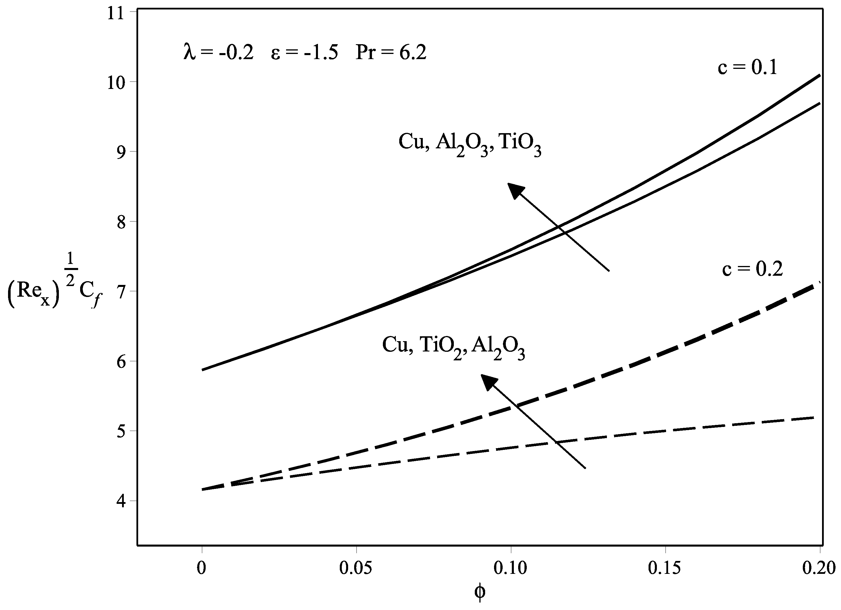
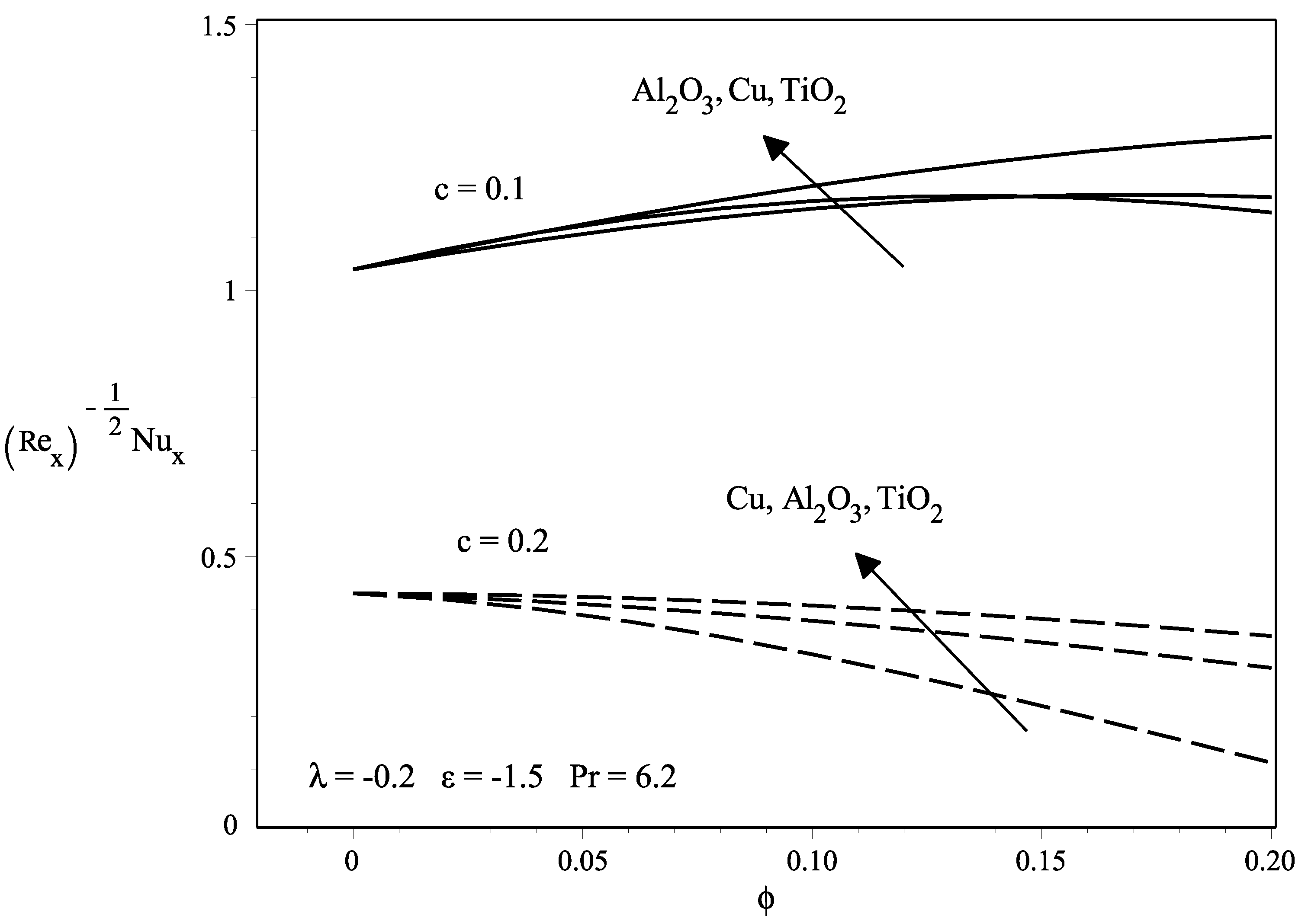
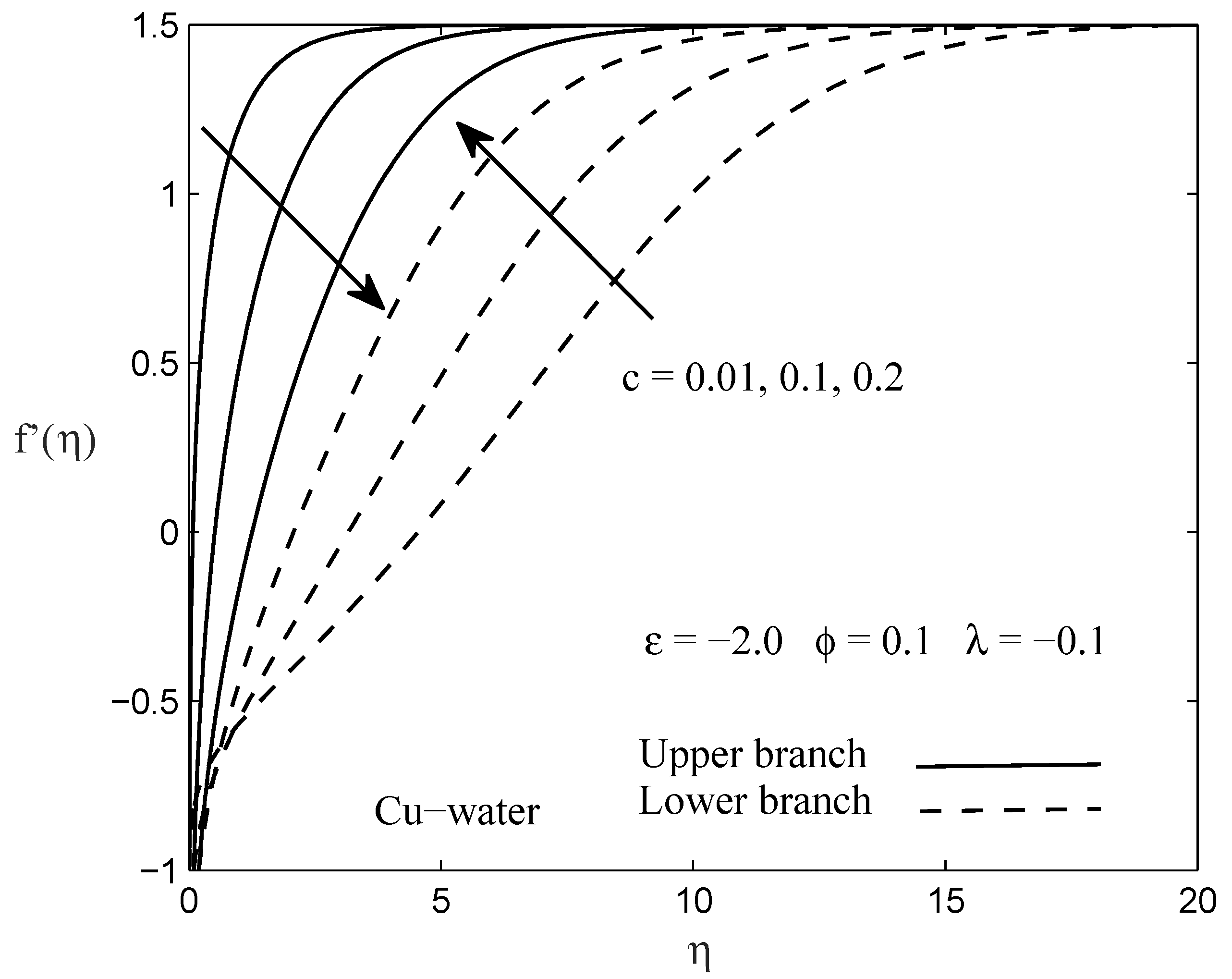
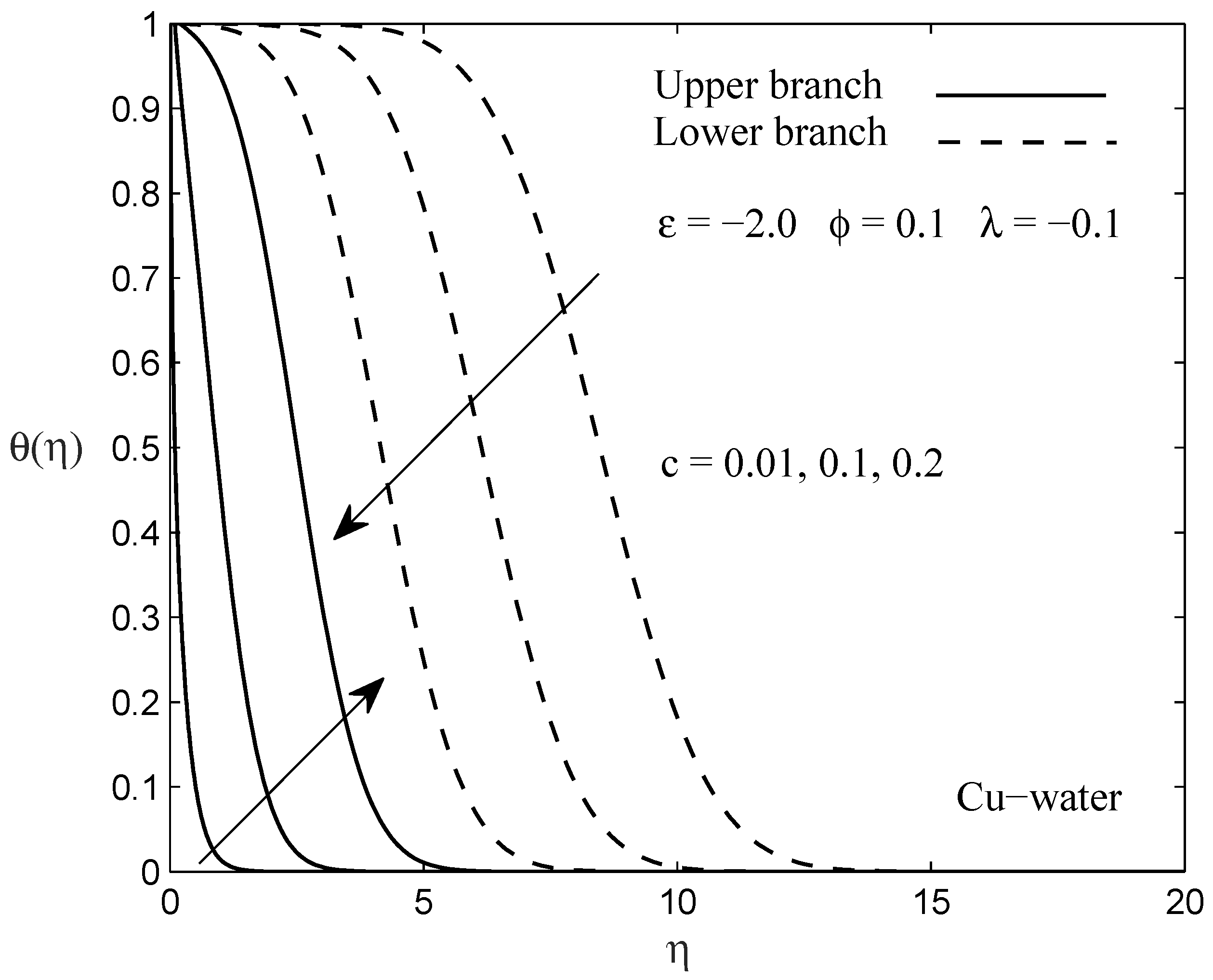
• The magnitude of the skin friction coefficient and the local Nusselt number increases as the size of the needle decreases. The thinner surface of the needle causes the heat to be easily diffused, hence reducing the drag force between the needle and the free stream.
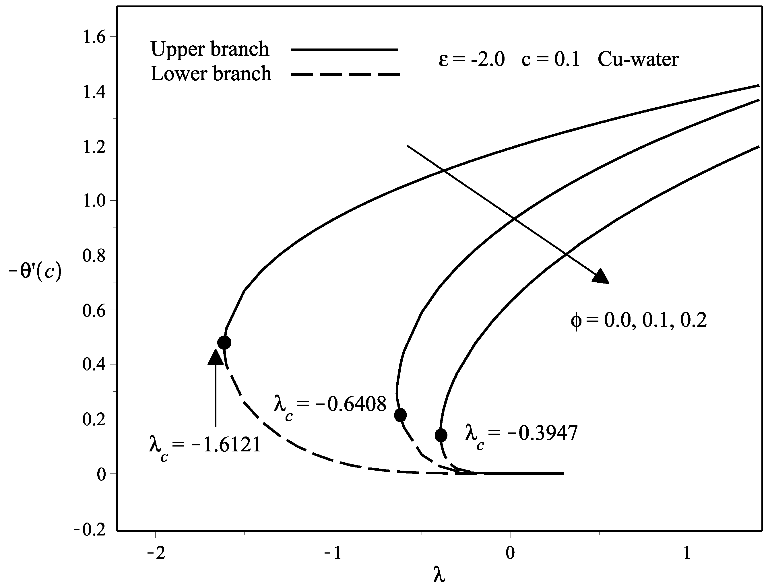
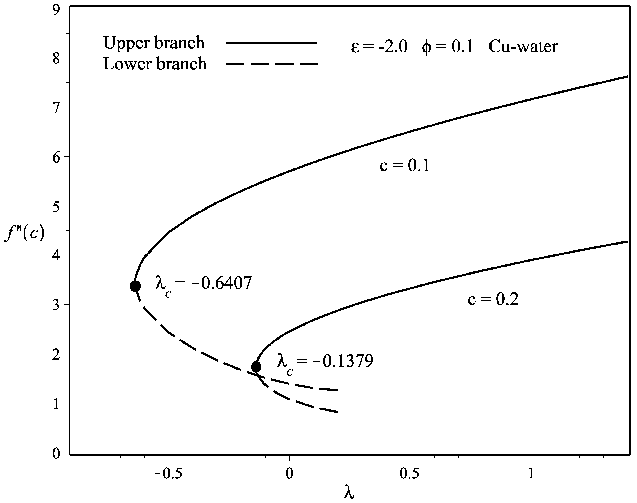
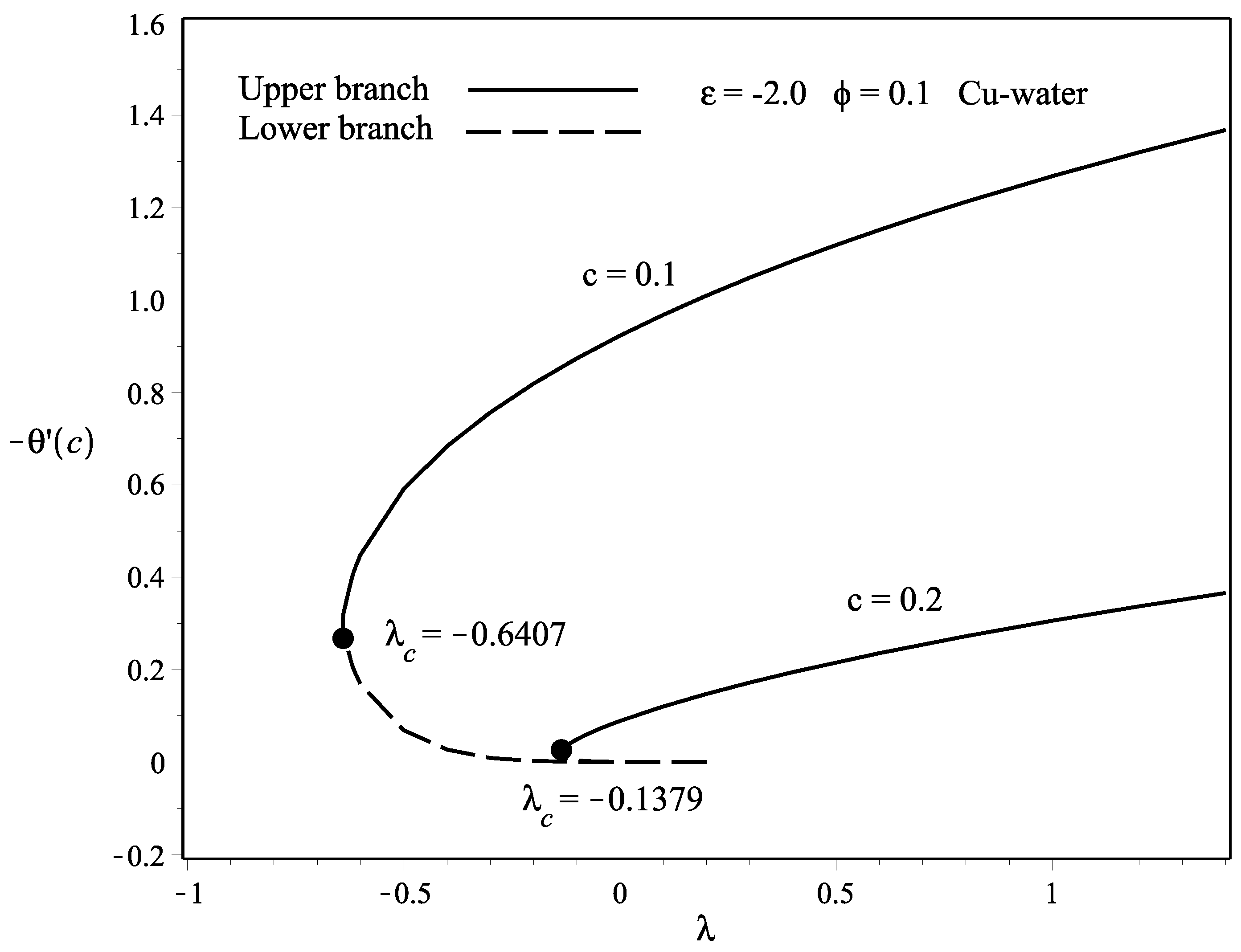
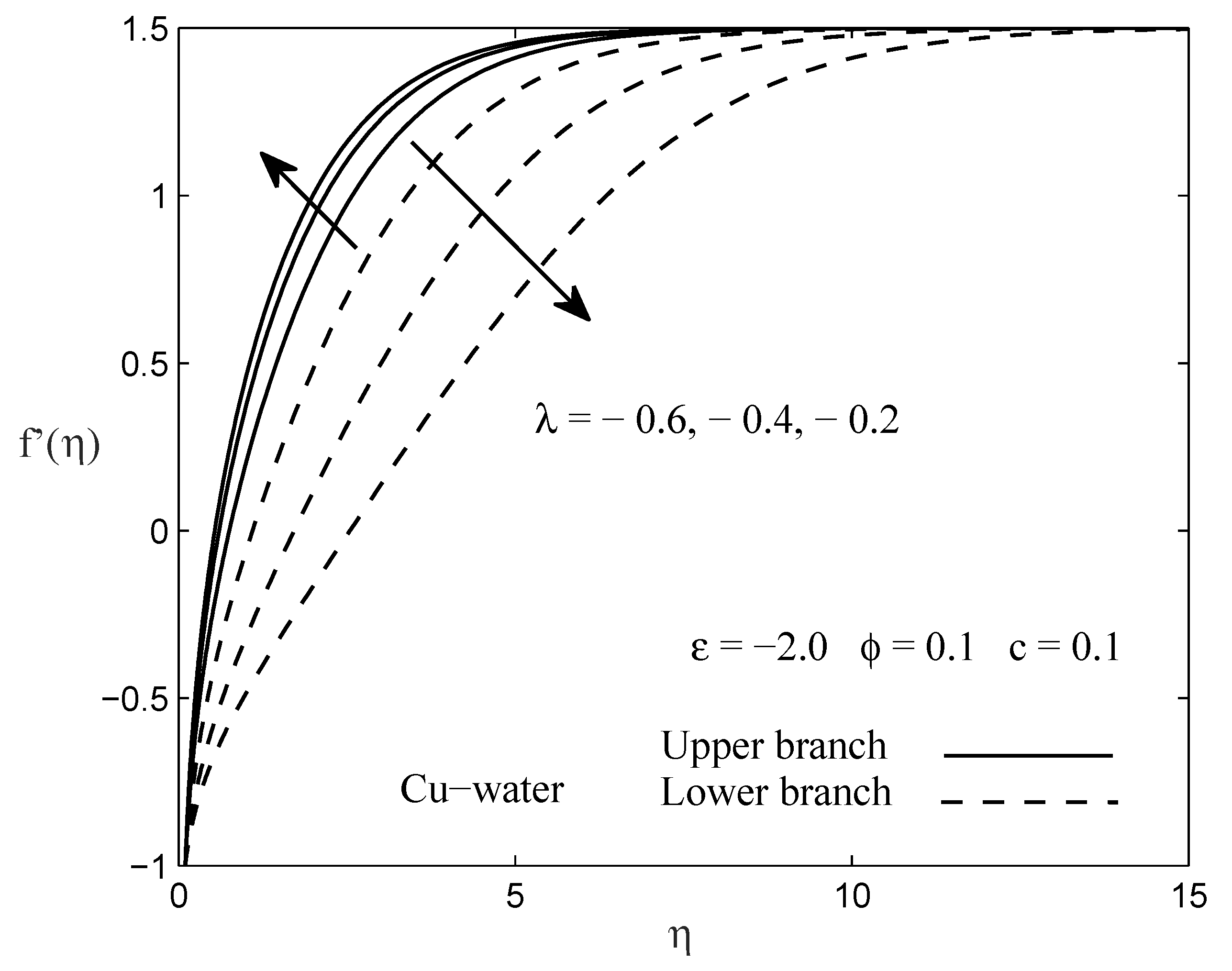
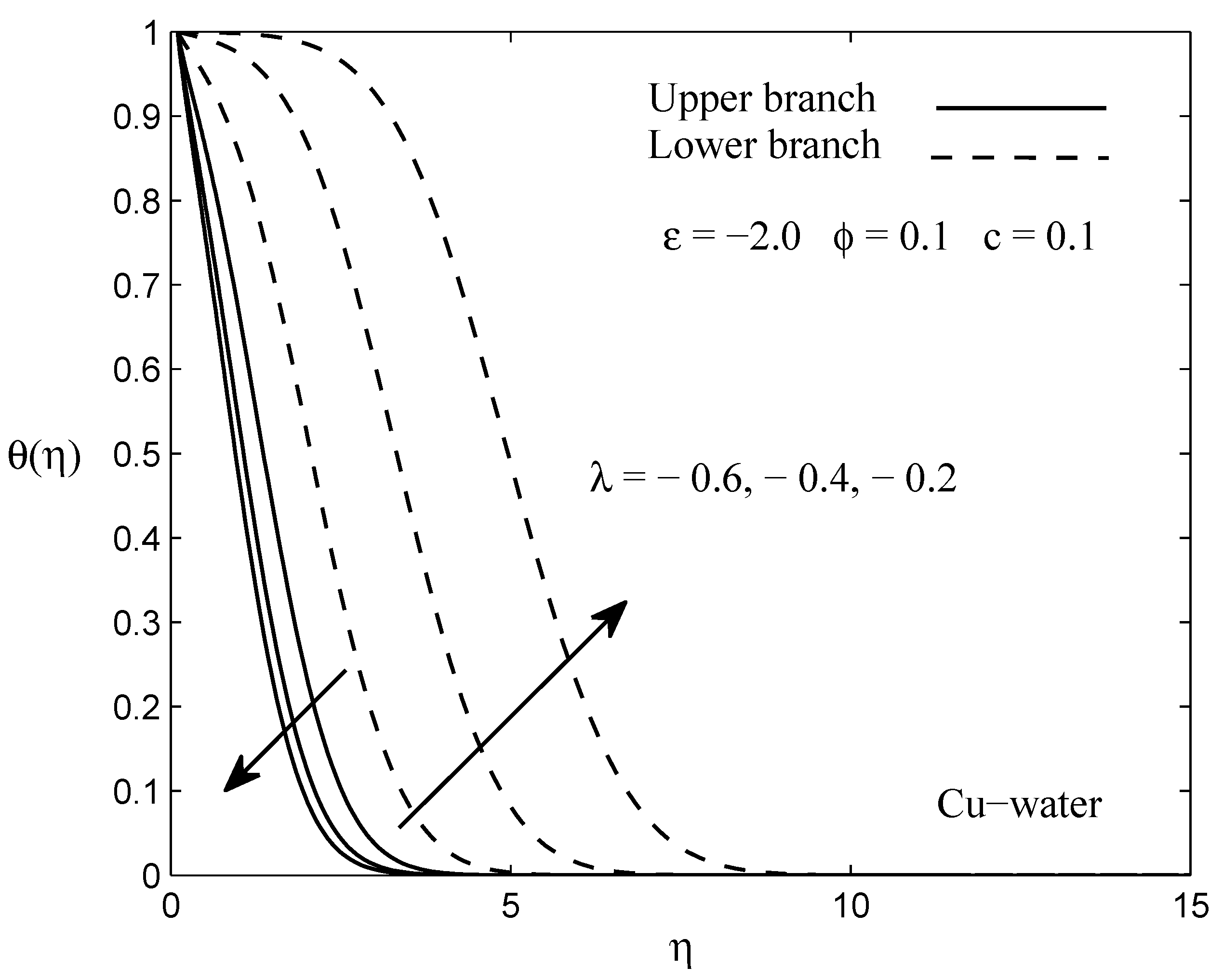
• The existence of the dual solutions occurs when the needle and the fluid move in the opposite way ($\epsilon <0$), while the solution is unique when they move in the same way ($\epsilon >0$). Nevertheless, the range of the dual solutions exists only in between ${\epsilon }_c<\epsilon \le 0$.
• The presence of the nanoparticles volume fraction in the flow causes the skin friction coefficient, as well as the heat transfer rate on the needle surface to increase especially for the thinner surface.
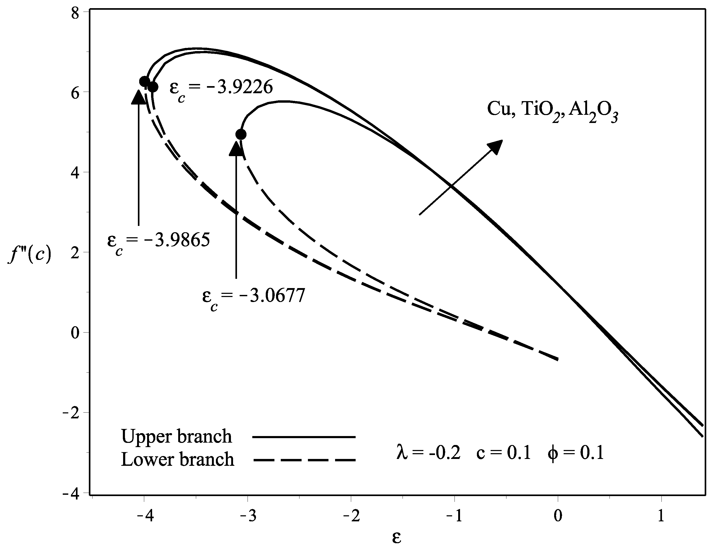
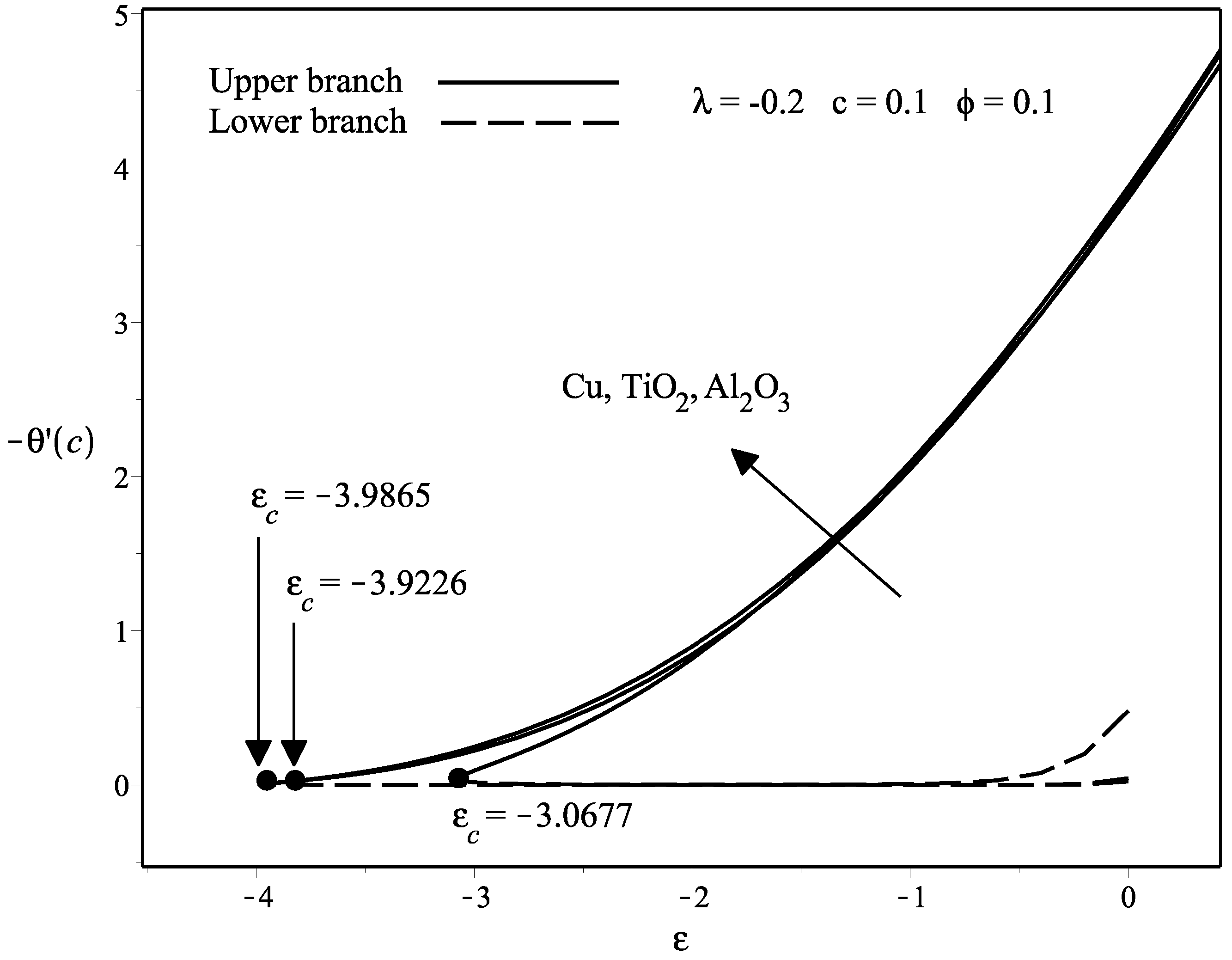
• The dual solutions are more pronounced when the flow is opposing ($\lambda <0$) and the range is between ${\lambda }_c<\lambda \le 0.3$. When $\lambda <{\lambda }_c$, no solutions are obtained.
• The stability analysis has confirmed that the upper branch solution is stable, while the lower branch solution is unstable by observing the positive and negative sign of the eigenvalues obtained.

References

1. Choi, S.U.S. Enhancing thermal conductivity of fluids with nanoparticles. Am. Soc. Mech. Eng. Fluids Eng. Div. 1995, 231, 99–105. [Google Scholar]
2. Wong, K.V.; Leon, O.D. Applications of Nanofluids: Current and Future. Adv. Mech. Eng. 2010, 2010, 519659. [Google Scholar] [CrossRef]
3. Saidur, R.; Leong, K.Y.; Mohammad, H.A. A review on applications and challenges of nanofluids. Renew. Sustain. Energy Rev. 2011, 15, 1646–1668. [Google Scholar] [CrossRef]
4. Huminic, G.; Huminic, A. Application of nanofluids in heat exchangers: A review. Renew. Sustain. Energy Rev. 2012, 16, 5625–5638. [Google Scholar] [CrossRef]
5. Khanafer, K.; Vafai, K.; Lightstone, M. Buoyancy-driven heat transfer enhancement in a two-dimensional enclosure utilizing nanofluids. Int. J. Heat Mass Trans. 2003, 46, 3639–3653. [Google Scholar] [CrossRef]
6. Buongiorno, J. Convective transport in nanofluids. J. Heat Trans. 2006, 128, 240–250. [Google Scholar] [CrossRef]
7. Tiwari, R.K.; Das, M.K. Heat transfer augmentation in a two-sided lid-driven differentially heated square cavity utilizing nanofluids. Int. J. Heat Mass Trans. 2007, 50, 2002–2018. [Google Scholar] [CrossRef]
8. Nield, D.A.; and Kuznetsov, A.V. The Cheng–Minkowycz problem for natural convective boundary-layer flow in a porous medium saturated by a nanofluid. Int. J. Heat Mass Trans. 2009, 52, 5792–5795. [Google Scholar] [CrossRef]
9. Kuznetsov, A.V.; Nield, D.A. The onset of double-diffusive nanofluid convection in a layer of a saturated porous medium. Transp. Porous Med. 2010, 85, 941–951. [Google Scholar]
10. Brinkman, H.C. The viscosity of concentrated suspensions and solutions. J. Chem. Phys. 1952, 20, 571–581. [Google Scholar] [CrossRef]
11. Jalilpour, B.; Jafarmadar, S.; Ganji, D.D.; Shotorban, A.B.; Taghavifar, H. Heat generation/absorption on MHD stagnation flow of nanofluid towards a porous stretching sheet with prescribed surface heat flux. J. Mol. Liq. 2004, 195, 194–204. [Google Scholar] [CrossRef]
12. Bachok, N.; Ishak, A.; Pop, I. Boundary-layer flow of nanofluids over a moving surface in a flowing fluid. Int. J. Therm. Sci. 2010, 49, 1663–1668. [Google Scholar] [CrossRef]
13. Reddy, C.R.; Murthy, P.V.S.N.; Chamkha, A.J.; Rashad, A.M. Soret effect on mixed convection flow in a nanofluid under convective boundary condition. Int. J. Heat Mass Trans. 2013, 64, 384–392. [Google Scholar] [CrossRef]
14. Roşca, N.C.; Pop, I. Unsteady boundary layer flow of a nanofluid past a moving surface in an external uniform free stream using Buongiorno’s model. Comput. Fluids 2014, 95, 49–55. [Google Scholar] [CrossRef]
15. Lee, L.L. Boundary layer over a thin needle. Phys. Fluids 1967, 10, 1820–1822. [Google Scholar] [CrossRef]
16. Narain, J.P.; Uberoi, S.M. Combined forced and free-convection heat transfer from vertical thin needles in a uniform stream. Phys. Fluids 1972, 15, 1879–1882. [Google Scholar] [CrossRef]
17. Narain, J.P.; Uberoi, S.M. Combined forced and free-convection over thin needles. Int. J. Heat Mass Trans. 1973, 16, 1505–1512. [Google Scholar] [CrossRef]
18. Wang, C.Y. Mixed convection on a vertical needle with heated tip. Phys. Fluids 1990, 2, 622–625. [Google Scholar] [CrossRef]
19. Ishak, A.; Nazar, R.; Pop, I. Boundary layer flow over a continuously moving thin needle in a parallel free stream. Chin. Phys. Lett. 2007, 24, 2895–2897. [Google Scholar] [CrossRef]
20. Ahmad, S.; Arifin, N.M.; Nazar, R.; Pop, I. Mixed convection boundary layer flow along vertical thin needles: Assisting and opposing flows. Int. Commun. Heat Mass Trans. 2008, 35, 157–162. [Google Scholar] [CrossRef]
21. Afridi, M.I.; Qasim, M. Entropy generation and heat transfer in boundary layer flow over a thin needle moving in a parallel stream in the presence of nonlinear Rosseland radiation. Int. J. Therm. Sci. 2018, 123, 117–128. [Google Scholar] [CrossRef]
22. Grosan, T.; Pop, I. Forced Convection Boundary Layer Flow Past Nonisothermal Thin Needles in Nanofluids. J. Heat Trans. 2011, 133. [Google Scholar] [CrossRef]
23. Hayat, T.; Khan, M.I.; Farooq, M.; Yasmeen, T.; Alsaedi, A. Water-carbon nanofluid flow with variable heat flux by a thin needle. J. Mol. Liq. 2016, 224, 786–791. [Google Scholar] [CrossRef]
24. Soid, S.K.; Ishak, A.; Pop, I. Boundary layer flow past a continuously moving thin needle in a nanofluid. Appl. Therm. Eng. 2017, 114, 58–64. [Google Scholar] [CrossRef]
25. Krishna, P.M.; Sharma, R.P.; Sandeep, N. Boundary layer analysis of persistent moving horizontal needle in Blasius and Sakiadis magnetohydrodynamic radiative nanofluid flows. Nucl. Eng. Technol. 2017, 49, 1654–1659. [Google Scholar] [CrossRef]
26. Ahmad, R.; Mustafa, M.; Hina, S. Buongiorno’s model for fluid flow around a moving thin needle in a flowing nanofluid: A numerical study. Chin. J. Phys. 2017, 55, 1264–1274. [Google Scholar] [CrossRef]
27. Trimbitas, R.; Grosan, T.; Pop, I. Mixed convection boundary layer flow along vertical thin needles in nanofluids. Int. J. Numer. Methods Heat Fluid Flow 2014, 24, 579–594. [Google Scholar] [CrossRef]
28. Sparrow, E.M.; Abraham, J.P. Universal solutions for the streamwise variation of the temperature of a moving sheet in the presence of a moving fluid. Int. J. Heat Mass Trans. 2005, 48, 3047–3056. [Google Scholar] [CrossRef]
29. Abraham, J.P.; Sparrow, E.M. Friction drag resulting from the simultaneous imposed motions of a freestream and its bounding surface. Int. J. Heat Fluid Flow 2005, 26, 289–295. [Google Scholar] [CrossRef]
30. Oztop, H.F.; Abu-Nada, E. Numerical study of natural convection in partially heated rectangular enclosures filled with nanofluids. Int. J. Heat Fluid Flow 2008, 29, 1326–1336. [Google Scholar] [CrossRef]
31. Weidman, P.D.; Kubitschek, D.G.; Davis, A.M.J. The effect of transpiration on self-similar boundary layer flow over moving surfaces. Int. J. Eng. Sci. 2006, 44, 730–737. [Google Scholar] [CrossRef]
32. Harris, S.D.; Ingham, D.B.; Pop, I. Mixed convection boundary-layer flow near the stagnation point on a vertical surface in a porous medium: Brinkman model with slip. Transp. Porous Media 2009, 77, 267–285. [Google Scholar] [CrossRef]
Figure 1. Physical models and coordinate systems: (a) assisting flow and (b) opposing flow.
Applsci 08 00842 g001
Figure 2. Effect of mixed convection parameter λ on the variation of shear stress for various values of nanoparticle volume fraction ϕ .
Applsci 08 00842 g002
Figure 3. Effect of mixed convection parameter λ on the variation of local heat flux for various values of nanoparticle volume fraction ϕ .
Applsci 08 00842 g003
Figure 4. Effect of the velocity ratio parameter ε on the variation of shear stress for different nanoparticles.
Applsci 08 00842 g004
Figure 5. Effect of the velocity ratio parameter ε on the variation of local heat flux for different nanoparticles.
Applsci 08 00842 g005
Figure 6. Effect of mixed convection parameter λ on the variation of shear stress for different needle sizes c.
Applsci 08 00842 g006
Figure 7. Effect of mixed convection parameter λ on the variation of local heat flux for different needle sizes c.
Applsci 08 00842 g007
Figure 8. Variation of skin friction coefficients with nanoparticle volume fraction ϕ for different nanoparticles when c = 0 . 1 and c = 0 . 2 .
Applsci 08 00842 g008
Figure 9. Variation of local Nusselt numbers with nanoparticle volume fraction ϕ for different nanoparticles when c = 0 . 1 and c = 0 . 2 .
Applsci 08 00842 g009
Figure 10. Effect of needle size c on the variation of velocity profiles.
Applsci 08 00842 g010
Figure 11. Effect of needle size c on the variation of temperature profiles.
Applsci 08 00842 g011
Figure 12. Effect of mixed convection parameter λ on the variation of velocity profiles.
Applsci 08 00842 g012
Figure 13. Effect of mixed convection parameter λ on the variation of temperature profiles.
Applsci 08 00842 g013