Parallel Improvements of the Jaya Optimization Algorithm

Abstract

A wide range of applications use optimization algorithms to find an optimal value, often a minimum one, for a given function. Depending on the application, both the optimization algorithm’s behavior, and its computational time, can prove to be critical issues. In this paper, we present our efficient parallel proposals of the Jaya algorithm, a recent optimization algorithm that enables one to solve constrained and unconstrained optimization problems. We tested parallel Jaya algorithms for shared, distributed, and heterogeneous memory platforms, obtaining good parallel performance while leaving Jaya algorithm behavior unchanged. Parallel performance was analyzed using 30 unconstrained functions reaching a speed-up of up to $57.6x$ using 60 processors. For all tested functions, the parallel distributed memory algorithm obtained parallel efficiencies that were nearly ideal, and combining it with the shared memory algorithm allowed us to obtain good parallel performance. The experimental results show a good parallel performance regardless of the nature of the function to be optimized.

1. Introduction

Optimization algorithms aim at finding an optimal value for a given function within a constrained domain. However, functions to be optimized can be highly complex and may present different numbers of parameters (or design variables). Indeed, many functions have local minima, so finding the absolute optimal value among the whole range of possibilities can be difficult.

Optimization methods fall into two main categories: deterministic and heuristic approaches. Deterministic approaches take advantage of the problem’s analytical properties to generate a sequence of points that converge toward a global optimal solution, these methods depend heavily on linear algebra, since they are commonly based on the computation of the gradient of the response variables. Deterministic approaches can provide general tools for solving optimization problems to obtain a global or an approximate global optimum (see [1]). Nonetheless, in the case of non-convex or large-scale optimization problems, the issues can be so complex that deterministic methods may not allow one to easily derive a globally optimal solution within a reasonable time frame. These methods are within the scope of mathematical programming, being the results of a deterministic optimization process that is unequivocable and replicable. Well known methods include the Newton method, the gradient descent method, and the Broyden–Fletcher–Goldfarb–Shanno (BFGS) method. Heuristic methods are proposed in order to speed the convergence up, to avoid local minimums, and to avoid restrictions in the functions to be optimized. Heuristic methods can be defined as guided (random) search techniques that are able to produce an acceptable problem solution, though its adequacy with respect to the target problem cannot be formally proven.

Heuristic optimization algorithms are usually classified into two main groups: Evolutionary Algorithms (EA) and Swarm Intelligence (SI) algorithms. Among EA algorithms, worthy of mention are the Genetic Algorithm (GA), the Evolutionary Strategy (ES), Evolutionary Programming (EP), Genetic Programming (GP), Differential Evolution (DE), Bacteria Foraging Optimization (BFO), and the Artificial Immune Algorithm (AIA). Among SI algorithms, worthy of mention are Particle Swarm Optimization (PSO), Shuffled Frog Leaping (SFL), Ant Colony Optimization (ACO), Artificial Bee Colony (ABC), and the Fire Fly (FF) algorithm. Other algorithms based on phenomena in nature have been developed, and these include Harmony Search (HS), Lion Search (LS), the Gravitational Search Algorithm (GSA), Biogeography-Based Optimization (BBO), and the Grenade Explosion Method (GEM).

The success of the vast majority of these algorithms is largely based on the parameters they use, which basically guide the search process and contribute chiefly to exploring the search space. The proper tuning of an algorithm-specific parameters represents a crucial success factor toward finding the global optimum. There are other algorithm-specific parameters. In PSO, these include population size, maximum number of generations, elite size, inertia weight, and acceleration rate; in ABC, these include onlooker bees, employed bees, and scout bees; in HS, harmony memory, number of improvisations, and pitch adjusting rate.

Recently, two optimization algorithms, called TLBO (Teacher–Learner Based Optimization) [2] and Jaya [3], allowing one to dispense with specific parameter tuning have been put forward. In fact, only general parameters such as the number of iterations and population dimension are required. The TLBO and the Jaya algorithm are quite similar, the main difference being that TLBO uses two phases at every iteration (teacher and learner phases), while the Jaya algorithm performs only one. The Jaya algorithm in particular has sparked great interest that is growing within a range of diverse scientific areas, see [4,5,6,7,8,9,10,11,12,13,14,15,16,17] among others. Recently, modifications to the Jaya algorithm have been proposed, increasing the number of scientific application areas, and these modified algorithms include the elitist Jaya [18], the self Jaya [19], and the quasi-oppositional-based Jaya [20] algorithms.

Some recent works show the advantages of using parallel architectures when executing optimization algorithms. The authors of [21] implemented the TLBO algorithm on a multicore processor within an OpenMP (Open MultiProcessing) environment. The OpenMP strategy emulated the sequential TLBO algorithm exactly, so calculation of fitness, calculation of mean, calculation of best, and comparison of fitness functions remained the same, while small changes were introduced to achieve better results. A set of 10 test functions were evaluated when running the algorithm on a single core architecture, and were then compared on architectures ranging from 2 to 32 cores. They obtain average speed-up values of $4.9x$ and $6.4x$ with 16 and 32 processors, respectively.

The authors of [22] implemented the Dual Population Genetic Algorithm on a parallel architecture. This algorithm is based on the original GA, but the Dual Algorithm adds a reserve population so as to avoid premature convergence proper to this kind of algorithm. A set of 8 test functions were optimized. Although they obtain average speed-up values of $1.64x$ using both 16 and 32 processors.

The authors of [23,24] analyzed the performance of population-based meta-heuristics using MPI (Message Passing Interface), OpenMP, and hybrid MPI/OpenMP implementations in a workstation with a multicore processor to solve a vehicle routing problem. A speed-up near $2.5x$ was reached in some cases, although in other cases a speed-up of only $1.0x$ to $1.5x$ was obtained.

The authors of [25] present a parallel implementation of the ant colony optimization metaheuristic to solve an industrial scheduling problem in an aluminium casting centre. The number of processors was set from 1 to 16. Results indicated that maximum speed-up was achieved when using 8 processors, but speed-up decreased as the number of processors further increased. A maximum speed-up of $5.94$ is obtained using 8 processors, which goes down to $5.45$ when using 16 processors.

An field of intense work of the scientific community is artificial intelligence [26], in which neural-symbolic computation [27] is a key challenge, especially to construct computational cognitive models that admit integrated algorithms for learning and reasoning that can be treated computationally. Moreover, deep learning is not an optimization algorithm in itself, but the deep network has an objective function, so a heuristic optimization algorithm can be used to tune the network. Another important field is data mining that applies to scientific areas [28,29,30] a where Jaya can also be applied further; for example, in [31], data optimization techniques and data mining are used together to develop a hybrid optimization algorithm.

The above review of the state of the art shows that it is generally feasible to implement optimization techniques on a parallel architecture. However, there can be drawbacks in cases where implementations constrain the speed-up increment of parallel solutions when compared to sequential execution. Therefore, parallel implementation of these kinds of algorithms must be performed carefully to benefit from the advantages of parallel architectures.

We will now present in Section 2, the recent Jaya optimization algorithm and its advantages. In Section 3, we will describe the parallel algorithms that have been developed, and in Section 4, we analyze the latter both in terms of parallel performance and Jaya algorithm behavior. Conclusions are drawn in Section 5.

2. The Jaya Algorithm

We review here some different studies of the Jaya algorithm and summarize their conclusions. The author of in [3] tested the performance of the Jaya algorithm, by means of a series of experiments on 24 constrained benchmark problems. The goal of the algorithm was to get closer to the best solution, but in so doing it also moves away from the worst solution. Results obtained using the Jaya algorithm were compared with results obtained by other optimization algorithms such as GA, ABC, TLBO, and a few others. The superiority of Jaya was shown by means of two statistical tests: the Friedman rank test and the Holm–Sidak test. The Jaya algorithm came first in the case of the best and mean solutions for all considered benchmark functions, while TLBO came second. With regard to the results of the Friedman rank test for the Success Rate solutions obtained, Jaya again came first followed by TLBO. The Holm–Sidak test provided a difference index related to the results obtained by Jaya and the other algorithms. This test showed a maximal difference between Jaya on the one hand and GA and BBO on the other, and a minimal difference with TLBO.

In the same study, Jaya performance was tested further on 30 unconstrained benchmark functions that are well known in the literature on optimization. Results obtained using Jaya were compared with results obtained using other optimization algorithms such as GA, PSO, DE, ABC, and TLBO. Mean results obtained were compared with other algorithms. Jaya obtained better results in terms of best, mean, and worst values of each objective function and standard deviation.

The authors of [32] applied Jaya to 21 benchmark problems related to constrained design optimization. In addition to these problems, the algorithm’s performance was studied over four constrained mechanical design problems. An analysis of the results revealed that Jaya was superior to, or could compete with, the others when applied to the problems in question. The authors of [33] showed that Jaya is applicable to data clustering problems. Results demonstrated that the algorithm exhibited better performance in most of the considered real-time datasets and was able to cluster appropriate partitions. We want to emphasize that our parallel algorithms do not modify the behavior of the Jaya algorithm. Moreover, in [15], the authors explore the use of advanced optimization algorithms for determining optimum parameters for grating based sensors; in particular, Cuckoo search, PSO, TLBO, and Jaya algorithms were evaluated. The best performance was obtained using the Jaya algorithm, good results were also obtained using the Cuckoo search algorithm, but it should be noted that the latter requires tuning the specific parameters of the algorithm to find the global optimum value.

3. Parallel Approaches

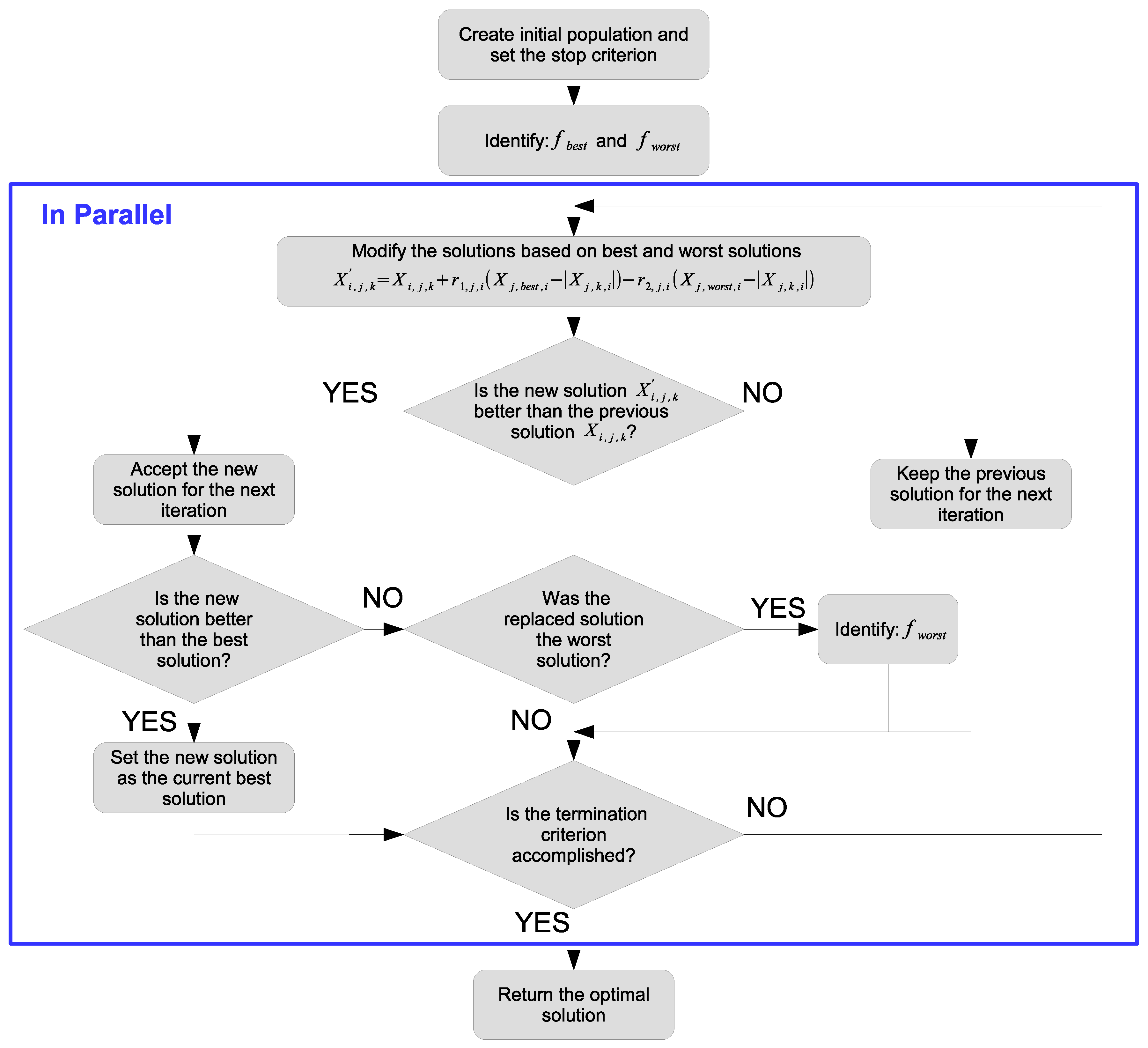
The parallel Jaya algorithm developed is shown in Figure 1. We will describe how the Jaya algorithm has been implemented in order to identify exploitable inherent sources of parallelism. Algorithm 1 shows the skeleton of the sequential implementation of the Jaya algorithm. The “Runs” parameter corresponds to the number of independent executions performed; therefore, in Line 26 of Algorithm 1, the different “Runs” solutions should be evaluated. First, for each independent execution, an initial population is computed (Lines 7–19), and, for each population member, VAR design variables can be obtained. It should be noted that the population size is an input parameter of the optimization algorithm, while the number of design variables is an intrinsic characteristic of the function to be optimized. The second input parameter is the number of “Iterations,” i.e., the number of new populations created based on the current population. Once a new population is created, each member of the current population is compared with its corresponding member of the new population, and is replaced if it improves the evaluation of the function. A detailed description of this procedure is shown in Algorithm 2.

As said, Algorithm 2 shows the main steps of the “Update Population” function (Line 21 of Algorithm 1), which is usually executed thousands, or tens of thousands, or hundreds of thousands of times; that is, almost all the computing time is consumed by said function.

Algorithm 1 Skeleton of the Jaya algorithm
1:	Define function to minimize
2:	Set $Runs$ parameter
3:	Set $Iterations$ parameter
4:	Set $PopulationSize$ parameter
5:	for$l=1$ to $Runs$ do
6:	Create New Population:
7:	for $i=1$ to $PopulationSize$ do
8:	for $j=1$ to $VARS$ do
9:	Obtain 2 random numbers
10:	Compute the design variable of the new member $Membe{r}_j^i$ {using Equation (1)}
11:	if $Membe{r}_j^i<MinValue$ then
12:	$Membe{r}_j^i=MinValue$
13:	end if
14:	if $Membe{r}_j^i>MaxValue$ then
15:	$Membe{r}_j^i=MaxValue$
16:	end if
17:	end for
18:	Compute and store $F(Membe{r}_j^i)$ {Function evaluation}
19:	end for
20:	for $l=1$ to $Iterations$ do
21:	Update Population
22:	end for
23:	Store Solution
24:	Delete Population
25:	end for
26:	Obtain Best Solution and Statistical Data

In Lines 20–24 of Algorithm 2, a new member is computed using the Jaya algorithm, i.e., using Equation (1). It should be noted that this computing uses both the current best and worst solution. In Equation (1), iterators j, k and i refer respectively to the design variable of the function, the member of the population, and the current iteration, while $r_{1,k,i}$ and $r_{2,k,i}$ are random numbers uniformly distributed.

$$x_{j,k,i}^{\prime }=x_{j,k,i}+r_{1,k,i}\left(x_{j,best,i}-\left|x_{j,k,i}\right|\right)-r_{2,k,i}\left(x_{j,worst,i}-\left|x_{j,k,i}\right|\right).$$

(1)

As said, the number of design variables for each member of each population (represented by “VAR” in Equation (2)) depends on the function to be optimized. In most of this study, we used the Rosenbrock function, as a test function, shown in Equation (2), where the number of design variables (VAR) is equal to 30. Regarding Algorithm 2, much of the computational cost corresponds to Lines 18–32. It should be noted that, in Line 22, the best and worst solutions are used, so this procedure depends on the i iteration. In Line 25 of Algorithm 2, the new member is evaluated using, for example, Equation (2), which corresponds to the Rosenbrock function. Naturally, the computational cost of Algorithm 2 can vary significantly depending on the function to be optimized. It should be noted that the total number of function evalutions depends on both the number of population updates (“Iterations” parameter) and the population size.

$$\begin{array}{c}\hfill F_{min}=\sum _{i=1}^{VAR}\left[100{\left(x_i^2-x_{i+1}\right)}^2+{\left(1-x_i\right)}^2\right].\end{array}$$

(2)

Algorithm 3 shows the skeleton of the shared memory parallel approach of Algorithm 1. Algorithm 3 focuses on the number of performed population updates (i.e., “Iterations”), distributing these population updates among the c available processes ($r=1,2,\dots ,c$). In Algorithm 3, ${\sum }_{r=1}^{c}Iteration{s}_r=Iterations$ must be satisfied, where $Iteration{s}_r$ is the number of population updates performed by process r, since a dynamic scheduling strategy has been used the number of populations updates per thread is not a fixed number. Since this algorithm has been designed for shared memory platforms, all solutions are stored in memory using OpenMP. Consequently, following parallel computation, the “sequential thread (or process)” obtains the best global solution and computes statistical values of all solutions obtained. As aforementioned, the number of iterations performed by each thread is not fixed, this number depends on the computational load assigned to each core in each particular execution, the automatic load balancing is implemented using the dynamic scheduling strategy of the OpenMP parallel loops. It should be noted that the total number of functions evaluations remains unchanged.

Algorithm 2 Update Population function of the Jaya algorithm
1:	Update Population:
2:	{
3:	{Obtain the current best and worst solution}
4:	$F^{worst}=F(Me{m}^1)$
5:	$Inde{x}^{worst}=1$
6:	$F^{best}=F(Me{m}^1)$
7:	$Inde{x}^{best}=1$
8:	for$k=2$ to $PopulationSize$ do
9:	if $F^{best}>F(Me{m}^k)$ then
10:	$Inde{x}^{best}=k$
11:	$F^{best}=F(Me{m}^k)$
12:	end if
13:	if $F^{worst}<F(Me{m}^k)$ then
14:	$Inde{x}^{worst}=k$
15:	$F^{worst}=F(Me{m}^k)$
16:	end if
17:	end for
18:	for$k=1$ to $PopulationSize$ do
19:	$old=k$
20:	for $j=1$ to $VARS$ do
21:	Obtain 2 random numbers
22:	Compute the design variable of the new member $New{M}_j$ {using Equation (1)}
23:	Check the bounds of $New{M}_j$
24:	end for
25:	Compute $F(NewM)$ {Function evaluation}
26:	if $F(NewM)<F(Me{m}^{old})$ then
27:	{Replace solution}
28:	for $j=1$ to $VARS$ do
29:	$Me{m}_j^{old}=New{M}_j$
30:	end for
31:	end if
32:	end for
33:	{Search for current best and worst solution as in Lines 4–17}
34:	}

Regarding Algorithms 2 and 3, data dependencies exist in the “Update Population” function solved in Algorithm 4, which shows the parallel “Update Population” function used in Algorithm 1. It should be noted that, to solve these data dependencies, Algorithm 4 includes up to 2 flush memory operations (Lines 3 and 35) and up to 3 critical sections (Lines 18, 26, and 44). It should be noted that only the “flush” procedure of Line 3 is performed in all iterations, and the rest of the flush and critical sections depends on the particular and non-deterministic computation. An analysis of data dependencies of the “Update Population” function reveals that its corresponding parallel function must be designed for shared memory platforms. It should be noted that the “flush” operations are performed to ensure that all threads have the same view of memory variables in which current best and worst solutions are stored. Furthermore, critical sections are used to avoid hazards in memory accesses. Some optimizations have been implemented in Algorithm 4, improving both the computational performance and the Jaya algorithm behavior. On the one hand, in Line 25 of Algorithm 4, when a new global minimum is obtained, it is quasi immediately used by all processes; on the other hand, in Line 34, the search of the current worst member is performed only by the thread that has removed the previous worst element.

Algorithm 3 Skeleton of shared memory parallel Jaya algorithm.
1:	for$l=1$ to $Runs$ do
2:	Parallel region:
3:	{
4:	Create New Population {Lines 7–19 of Algorithm 1}
5:	parallel for $i=1$ to $Iterations$ do
6:	Update Population
7:	end for
8:	Store Solution
9:	Delete Population
10:	}
11:	end for
12:	Sequential thread:
13:	Obtain Best Solution and Statistical Data

With respect to Algorithm 4, the computational load of one execution of the “Update Population” function might not be significant, depending on the computational cost of the function evaluation (Line 16), which obviously depends on the particular function to be optimized. For example, in Equation (2), the number of floating point operations is 7 for each iteration of the sum, so only 239 floating point operations have to be performed in each evaluation. Therefore, it is important to reduce both “flush” processes and “critical” sections, and it should be noted that we have developed the parallel algorithm avoiding synchronization points. Reducing both the “flush” procedures and the critical sections besides the automatic load balancing allows one to obtain good results both in efficiency and scalability. It is worth noting that, due to the large number of iterations performed, any poorly designed or implemented detail in the parallel proposal can significantly worsenboth the parallel performance and scalability.

As will be confirmed in Section 4, the good parallel behavior of the shared memory proposal of the Jaya optimization algorithm encourage the development of a parallel algorithm to be executed in clusters, in order to be able to efficiently increase the number of processes, reducing, drastically, the computing time. In order to use heterogeneous memory platforms (clusters) on the one hand, we must to identify a high-level inherent parallelism; on the other hand, we must to develop a hybrid memory model algorithm.

As explained in Section 2, and as can be seen in Algorithm 1, the Jaya algorithm performs several fully independent executions (“Runs”). Therefore, the Jaya algorithm offers great inherent parallelism at a higher level, but a key aspect must be the load balance. As aforementioned, we have developed a shared memory algorithm in which we have not used synchronization points and we have implemented techniques to ensure computational load balancing. The high-level parallel algorithm must accomplish these objectives and must be able to include the previously described algorithm.

The high-level parallel Jaya algorithm exploits the fact that all iterations of Line 5 in Algorithm 1 are actually independent executions. Therefore, the total number of executions (“Runs”) to be performed is divided among p available processes, taking into account, however, that it cannot be distributed statically. The high-level parallel algorithm must be designed for distributed memory platforms using MPI: on the one hand, we must to develop a load balance procedure; on the other hand, a final data gathering process (data collection from all processes) must be performed.

Algorithm 4 Update Population function of the shared memory parallel Jaya algorithm
1:	Update Population:
2:
3:	Flush operation over population and best and worst indices
4:	for$k=1$ to $PopulationSize$ do
5:	$old=k$
6:	for $j=1$ to $VARS$ do
7:	Obtain 2 random numbers
8:	Compute the design variable of the new member $New{M}_j$
9:	if $New{M}_j<MinValue$ then
10:	$New{M}_j=MinValue$
11:	end if
12:	if $New{M}_j>MaxValue$ then
13:	$New{M}_j=MaxValue$
14:	end if
15:	end for
16:	Compute $F(NewM)$ {Function evaluation}
17:	if $F(NewM)<F(Me{m}^{old})$ then
18:	Critical section to:
19:	{
20:	{Replace solution}
21:	for $j=1$ to $VARS$ do
22:	$Me{m}_j^{old}=New{M}_j$
23:	end for
24:	}
25:	if $F(NewM)<F(Me{m}^{best})$ then
26:	Critical section to:
27:	$Inde{x}^{Best}=i$ {$Me{m}^{best}=NewM$
28:	end if
29:	if $Inde{x}_{worst}==k$ then
30:	$FlagUpdateWorst=1$
31:	end if
32:	end if
33:	end for
34:	if$FlagUpdateWorst==1$then
35:	Flush operation over population
36:	$FlagUpdateWorst=0$
37:	$F(Tem{p}^{worst})=F(Me{m}^1)$
38:	$IndexTem{p}^{worst}=1$
39:	for $k=2$ to $PopulationSize$ do
40:	if $F(Tem{p}^{worst})<F(Me{m}^k)$ then
41:	$IndexTem{p}^{worst}=k$
42:	end if
43:	end for
44:	Critical section to:
45:	$Inde{x}^{worst}=IndexTem{p}^{worst}$ {$Me{m}^{worst}=Me{m}^{IndexTem{p}^{worst}}$}
46:	end if

The hybrid MPI/OpenMP algorithm developed is shown in Algorithm 5 and will be analyzed on a distributed shared memory platform. First, it should be noted that, if the number of worker processes desired is equal to p, the total number of distributed memory processes will be $p+1$. This is because there is a critical process (distributed memory process) that will be in charge of distributing the independent executions among the p available working processes. We call it the work dispatcher. Although the work dispatcher process is critical, it will be running in one of the nodes with worker processes, as no significant overhead is introduced in the overall parallel algorithm performance. The work dispatcher will be waiting to receive a signal of work request from an idle worker process. When a particular worker process requests a new work (independent execution), the dispatcher will assign a new independent execution or send an end-of-work signal. In Lines 6–13 of Algorithm 5, it can be verified that the computational load of dispatcher process is negligible. In Lines 15–24 of Algorithm 5, the shared memory parallel Jaya algorithm is used, i.e., Algorithm 3 sets the “Runs” parameter to 1. The total number of processes is equal to $tp=p\ast c$, where p is the number of distributed memory worker processes (MPI processes) and c is the number of shared memory processes (OpenMP processes or threads). When distributed shared memory platforms (clusters) are used, they are probably heterogeneous multiprocessors, taking into account that the proposed algorithms include load balancing procedures at two levels and thatthe load balance is assured. It should be noted that, if the number of shared memory processes is equal to 1 ($c=1$), Algorithm 5 is a distributed memory algorithm, and, to work with the hybrid algorithm, the number of distributed memory processes must be equal to or greater than 2, i.e., one dispatcher process and at least one worker process. In all cases, only worker-distributedmemory processes spawn shared memory threads.

Algorithm 5 Hybrid parallel Jaya algorithm for distributed shared memory platforms
1:	Define function to minimize
2:	Set $Iterations$ parameter (input parameter)
3:	Set population size (input parameter)
4:	Obtain the number of distributed memory worker processes p (input parameter)
5:	if is work dispatcher process then
6:	for $l=1$ to $Runs$ do
7:	Receive idle worker process signal
8:	Send independent execution signal
9:	end for
10:	for $l=1$ to p do
11:	Receive idle worker process signal
12:	Send end of work signal
13:	end for
14:	else
15:	while true do
16:	Send idle worker process signal to dispatcher process
17:	if Signal is equal to end of work signal then
18:	Break while
19:	else
20:	Obtain the number of shared memory processes c
21:	Compute 1 run of shared memory parallel Jaya algorithm
22:	Store Solution
23:	end if
24:	end while
25:	end if
26:	Perform a gather operation to collect all the solutions
27:	Sequential thread of the root process:
28:	Obtain Best Solution and Statistical Data

4. Results and Discussion

In this section, we analyze the parallel Jaya algorithms, presented in Section 3. We analyze the parallel behavior and verify that the optimization performance of the Jaya algorithm slightly improves or remains unchanged with respect to the sequential algorithm. In order to perform the tests, we developed the reference algorithm, presented in [3], in C language to implement the parallel algorithms, and used the GCC v.4.8.5 compiler [34]. We choose MPI v2.2 [35] for the high-level parallel approach and OpenMP API v3.1 [36] for the shared memory parallel algorithm. The parallel platform used was composed of 10 HP Proliant SL390 G7 nodes, where each node was equipped with two Intel Xeon X5660 processors. Each X5660 included six processing cores at 2.8 GHz, and QDR Infiniband was used as the communication network.

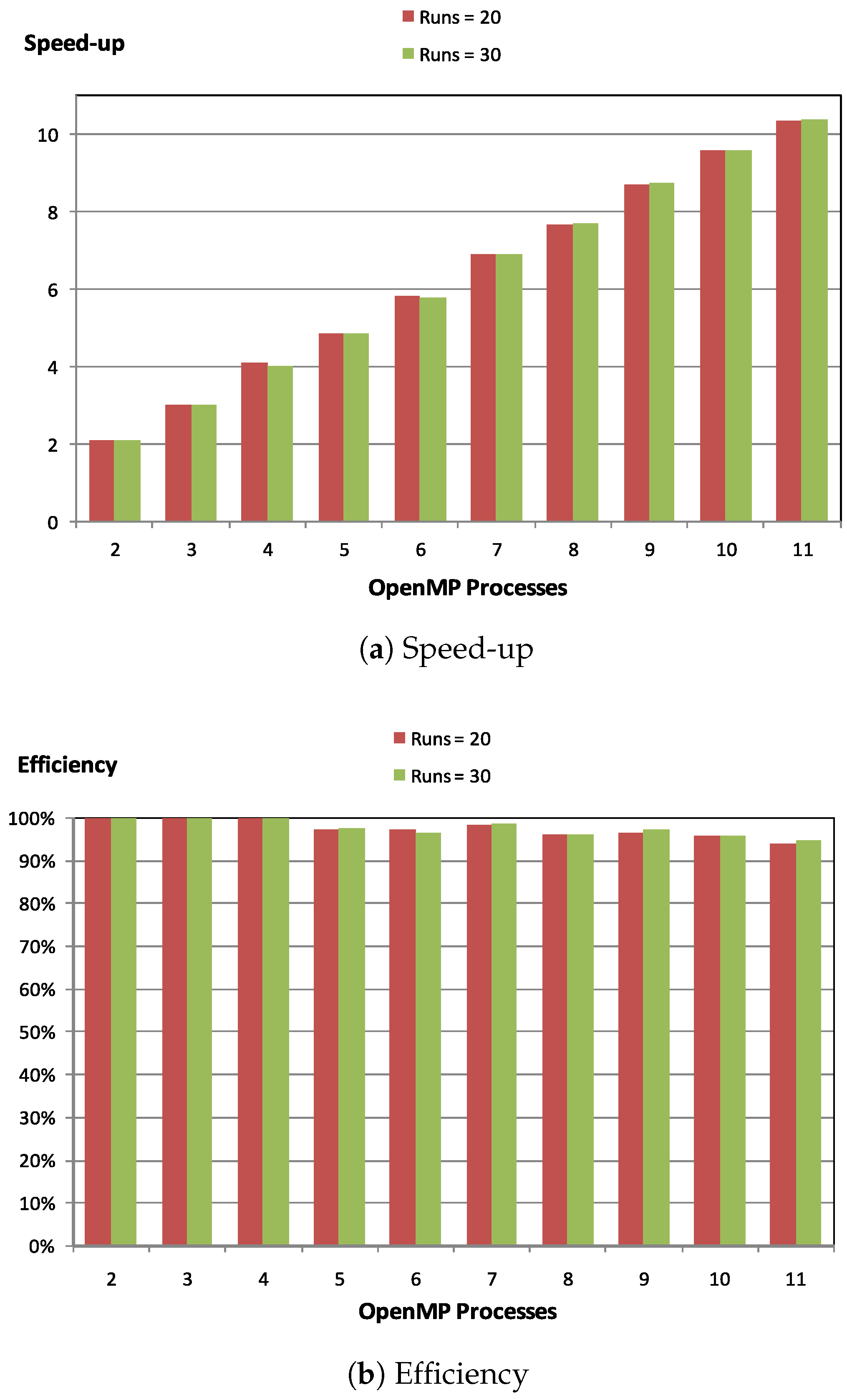
We will now analyze the parallel behavior of the parallel algorithm described in Algorithm 4, i.e., the shared memory parallel algorithm. Figure 2 shows results setting the “Iterations” parameter equal to 30,000 and using populations of 512 members. We observe that parallel efficiency being equal to, respectively, $100\%$ and $94\%$ when 2 and 11 processes are used, regardless of the value of “Runs.” We can conclude that, based on results presented in Figure 2, and applying the Rosenbrock function, for a population size equal to 512, the scalability is almost ideal.

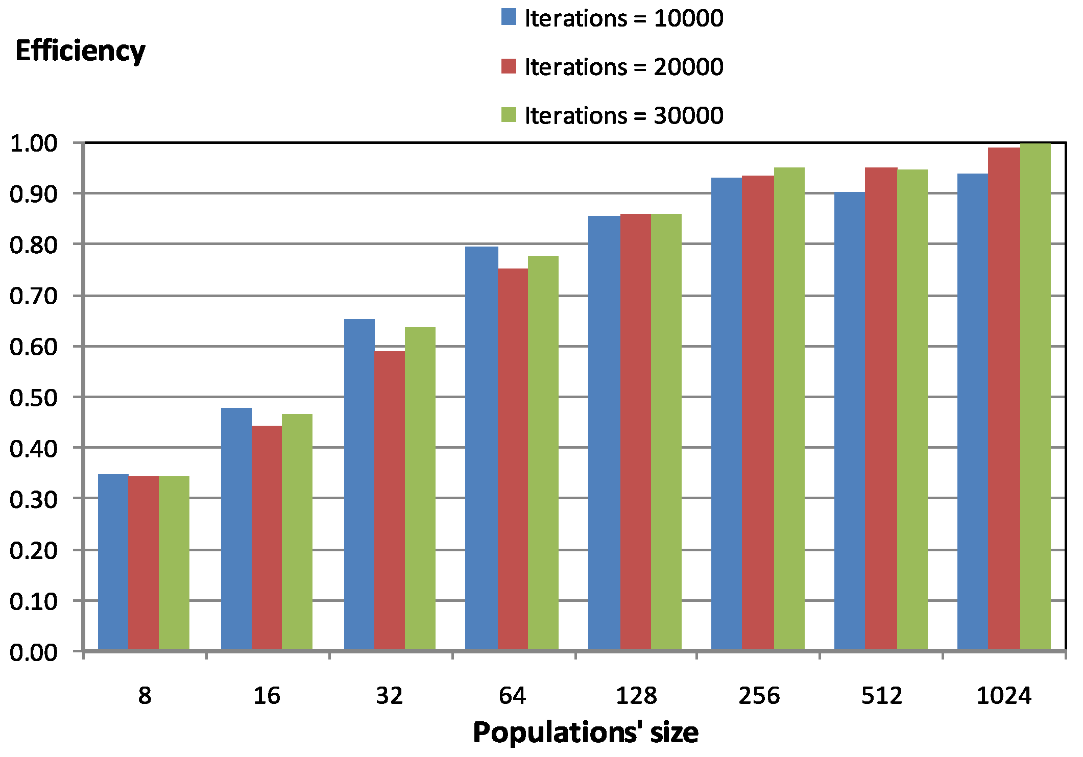
Figure 3 shows parallel behavior related to population size and number of iterations. Regarding both this figure and the rest of the experiments performed, the number of iterations does not affect parallel performance, while population size has been observed to be a critical parameter for obtaining good parallel performance. Results presented in Figure 3 indicate that, in order to obtain good parallel performance, population size must be greater than 64 members. In particular, in Figure 3, for population sizes greater than 128 members, the efficiency is always higher than $90\%$.

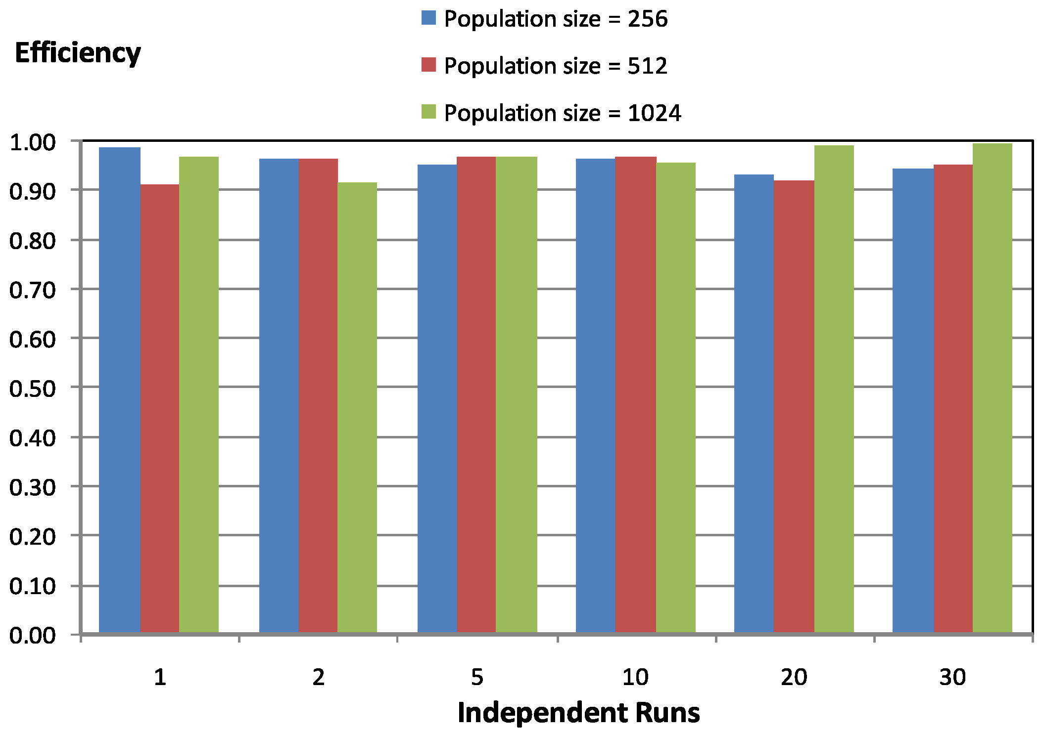
Figure 4 shows parallel behavior related to the number of independent executions, i.e., the number of different solutions obtained. As expected, the number of independent executions does not affect the parallel behavior of the shared memory parallel algorithm. We can conclude that the shared memory parallel algorithm obtains good parallel results with a minimum population size, and the rest of the parameters does not affect, or does so very slightly, the parallel performance.

The hybrid parallel algorithm developed combines the shared memory parallel algorithm analyzed and a high-level parallel algorithm based on the distribution, among nodes (multiprocessors), of the computing load associated with the independent executions that will be carried out. The latter, described in Algorithm 5, has been developed with MPI, the former with OpenMP. However, in order to efficiently use all processing units of the parallel platform we mapped, where possible, more than one MPI process was employed into one computing node. 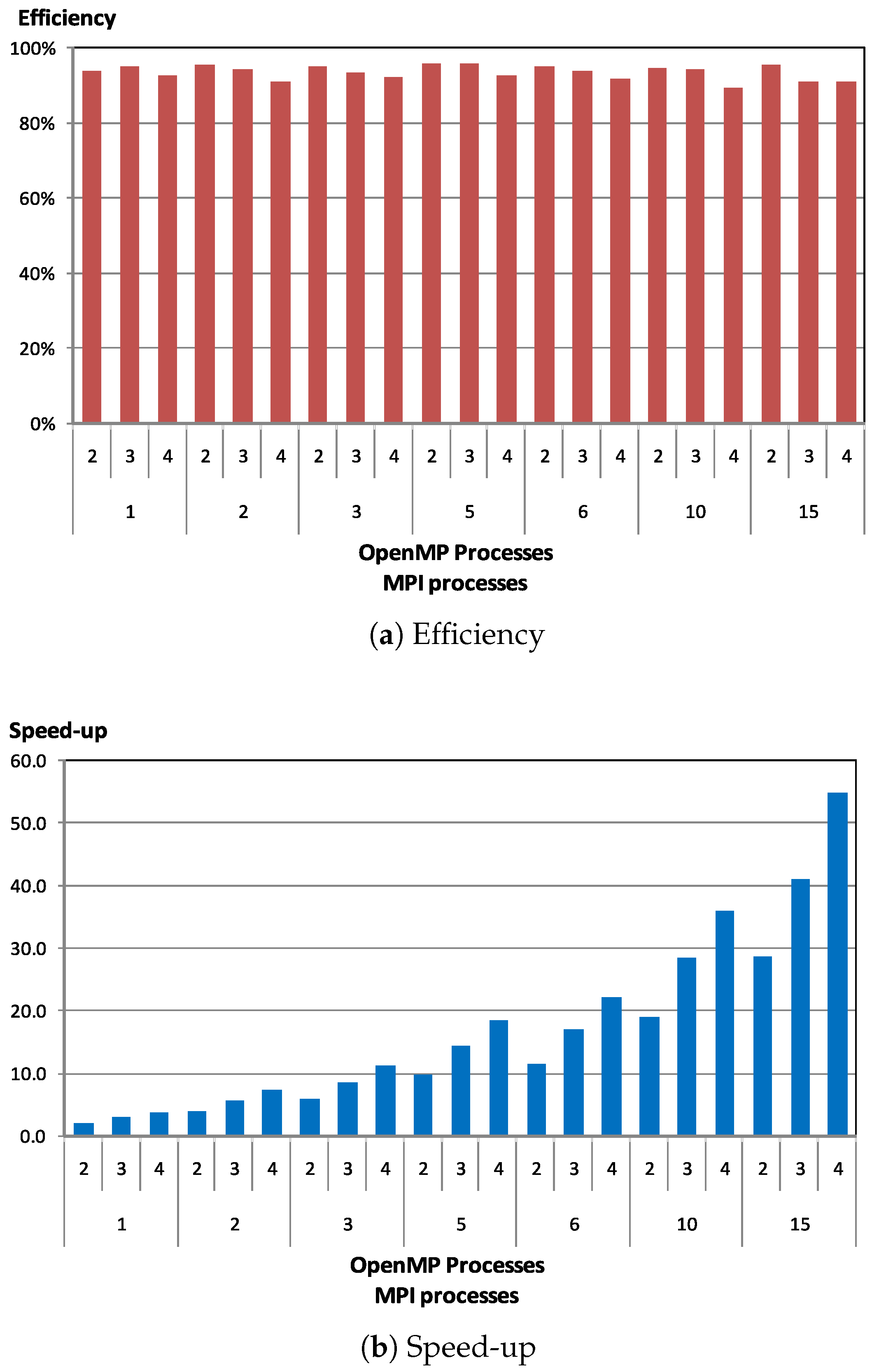Figure 5 shows the efficiency and speed-up for the hybrid parallel Jaya algorithm, executed in the heterogeneous memory platform previously described. It can be seen that the proposed hybrid parallel algorithm offers good scalability. It should be noted that we obtained a speed-up up to $54.6x$ using 60 processors of the heterogeneous memory platform. It is worth noting that the hybrid parallel algorithm exploits two levels of parallelism, and at both levels it includes load balancing mechanisms.

We must bear in mind that the execution of the Jaya algorithm is not a deterministic one, since Equation (1) depends on a random function. Each experiment in our study was performed by computing both the sequential and the parallel algorithm systematically and by verifying that the results obtained were almost identical; i.e., each parallel experiment was preceded by its corresponding sequential experiment, and we ensured that the difference between both optimal solutions exceeds ${10}^{-3}$. No errors were produced except for experiments with a very low number of function evaluations. On the other hand, in [3], the author performs an exhaustive analysis of the optimization performance of the Jaya algorithm.

To finish, we will analyze parallel behavior depending on the functions in question. We used the same benchmark functions as in [3] listed in

Table 1. Benchmark functions and their number of variables (VAR).

ID.	Function	VAR
F1	Sphere	30
F2	SumSquares	30
F3	Beale	5
F4	Easom	2
F5	Matyas	2
F6	Colville	4
F7	Trid 6	6
F8	Trid 10	10
F9	Zakharov	10
F10	Schwefel 1.2	30
F11	Rosenbrock	30
F12	Dixon-Proce	30
F13	Foxholes	2
F14	Branin	2
F15	Bohachevsky 1	2
F16	Booth	2
F17	Michalewicz 2	2
F18	Michalewicz 5	5
F19	Bohachevsky 2	2
F20	Bohachevsky 3	2
F21	GoldStein-Price	2
F22	Perm	4
F23	Hartman 3	3
F24	Ackley	30
F25	Penalized 2	30
F26	Langerman 2	2
F27	Langerman 5	5
F28	Langerman 10	10
F29	FletcherPowell 5	5
F30	FletcherPowell 10	10

.

Table 2. Sequential and parallel Jaya results. Population = 256. Iterations = 30,000. 10 MPI processes. 6 OpenMP processes. Runs = 30.

Function	Sequential Time (s)	Parallel Time (s)	Speed-Up	Efficiency
F1	126.0	2.58	48.9	81%
F2	129.9	2.67	48.6	81%
F3	108.5	2.02	53.7	90%
F4	26.7	0.50	53.7	90%
F5	70.2	1.42	49.3	82%
F6	18.4	0.41	44.6	74%
F7	26.6	0.53	50.0	83%
F8	44.7	0.87	51.6	86%
F9	67.7	1.55	43.7	73%
F10	254.9	4.85	52.6	88%
F11	131.9	2.46	53.7	90%
F12	132.4	2.44	54.2	90%
F13	999.9	17.59	56.8	95%
F14	16.3	0.33	49.9	83%
F15	17.3	0.34	51.0	85%
F16	9.4	0.23	41.4	69%
F17	54.9	1.05	52.5	87%
F18	171.8	3.15	54.5	91%
F19	12.4	0.26	48.2	80%
F20	16.2	0.32	51.1	85%
F21	12.0	0.27	44.3	74%
F22	330.3	5.74	57.6	96%
F23	45.5	0.81	56.1	94%
F24	465.6	8.21	56.7	95%
F25	583.8	10.25	56.9	95%
F26	82.9	1.54	53.7	90%
F27	474.4	8.57	55.3	92%
F28	1999.5	34.80	57.5	96%
F29	362.1	6.44	56.2	94%
F30	1471.8	25.81	57.0	95%

shows the results for all functions listed in Table 1, over 30 independent executions, 30,000 iterations, and populations of 256 members. Results shown in Table 2 are sequential computational time, parallel computational time, speed-up, and parallel efficiency, where 10 MPI processes and 6 OpenMP processes were used, i.e., using 60 processors of the parallel platform. It should be noted that, in general, all functions obtained good parallel behavior. In most cases, it is over $90\%$, and on average the efficiency is equal to $87\%$. Considering only functions with efficiency above the previous average, the average efficiency is $92\%$. We can increase the efficiency by decreasing the total number of processes used. It should also be noted that the sequential processing time does not exceed $12.0$ s.

Reducing the number of processes and leaving other parameters unchanged, parallel behavior improved as expected.

Table 3. Sequential and parallel Jaya results. Population = 256. Iterations = 30,000. 10 MPI processes. 2 OpenMP processes. Runs = 30.

Function	Sequential Time (s)	Parallel Time (s)	Speed-Up	Efficiency
F6	18.5	0.97	19.2	96%
F7	24.4	1.46	16.7	84%
F14	16.7	0.89	18.8	94%
F15	17.2	0.88	19.6	98%
F16	9.0	0.55	16.3	82%
F19	12.0	0.64	18.8	94%
F20	15.9	0.87	18.2	91%
F21	11.9	0.61	19.5	98%

shows results corresponding to Table 2, with only 2 OpenMP processes, i.e., using 20 processors, for those functions with lower computational cost. As can be seen in Table 3, efficiency values improve significantly, as anticipated, taking into account that high-level parallel algorithms offer better scalability.

It is worth noting that the parallel code has been fully optimized, thus improving parallel proposals of similar algorithms, and our hybrid proposal includes load balancing mechanisms at two levels. For example, in [21,22], parallelizing using OpenMP and using 8 processes, the maximum efficiency achieved is $55\%$ and $56\%$, respectively, while in the case of [23] it is only $23\%$. Under these conditions, our shared memory algorithm and our hybrid algorithm obtains an average efficiency higher than $90\%$. There is a recent algorithm, called HHCPJaya presented in [37], which obtains good results on both parallel and optimization performance. However, this algorithm has some drawbacks: it does not seem to be a general optimization algorithm, that is, the function to be optimized must be coded according to the partition at the level of the design variable performed, for example, a function such as the “Dixon-Price” function cannot be encoded using its general formulation. The method seems deterministic and not heuristic, because the seed used is always the same and does not use a random function; the method uses a deterministic function to generate the sequence of random numbers. When the random function is used instead, the deterministic function the method shows poor scalability. We present results using worker processes of up to 60. In our implementation, each of these processes uses a different seed for the generation of the sequence of random numbers; on the other hand, our algorithms need neither hyperpopulations nor functions with a large number of design variables.

Finally,

Table 4. Sequential and parallel Jaya solutions. Population = 64. Iterations = 1000. 5 MPI processes. Runs = 30.

Function	Optimum	OpenMP Processes	Best Parallel	Best Sequential	OpenMP Processes	Best Parallel	Best Sequential
F1	0.00000	2	0.00030	0.00163	6	0.00096	0.00233
F2	0.00000	2	0.00006	0.00018	6	0.00019	0.00048
F3	0.00000	2	0.00000	0.00000	6	0.00000	0.00000
F4	−1.00000	2	−1.00000	−1.00000	6	−1.00000	−1.00000
F5	0.00000	2	0.00000	0.00000	6	0.00000	0.00000
F6	0.00000	2	0.00008	0.00021	6	0.00022	0.00018
F7	−50.00000	2	−50.00000	−50.00000	6	−50.00000	−50.00000
F8	−210.00000	2	−210.00000	−210.00000	6	−210.00000	−210.00000
F9	0.00000	2	0.00017	0.00027	6	0.00003	0.00036
F10	0.00000	2	0.00002	0.00033	6	0.00026	0.00054
F11	0.00000	2	7.71880	24.31500	6	13.37600	33.43700
F12	0.00000	2	0.67569	0.69369	6	0.67506	0.72603
F13	0.99800	2	357.46000	498.07000	6	10.73000	200.70000
F14	0.39800	2	0.39789	0.39789	6	0.39789	0.39789
F15	0.00000	2	0.00000	0.00000	6	0.00000	0.00000
F16	0.00000	2	0.00000	0.00000	6	0.00000	0.00000
F17	−1.80130	2	−1.80130	−1.80130	6	−1.80130	−1.80130
F18	−4.68770	2	−4.68770	−4.68770	6	−4.68770	−4.68770
F19	0.00000	2	0.00000	0.00000	6	0.00000	0.00000
F20	0.00000	2	0.00000	0.00000	6	0.00000	0.00000
F21	3.00000	2	3.00000	3.00000	6	3.00000	3.00000
F22	0.00000	2	0.00343	0.00479	6	0.00175	0.00271
F23	−3.86000	2	−3.86280	−3.86280	6	−3.86280	−3.86280
F24	0.00000	2	0.00683	0.02936	6	0.02452	0.04375
F25	0.00000	2	0.00018	0.00107	6	0.00025	0.00113
F26	−4.15580	2	−4.15580	−4.15580	6	−4.15580	−4.15580
F27	−3.34260	2	−3.31040	−3.30630	6	−3.31760	−3.30780
F28	−3.15430	2	−3.06370	−3.06080	6	−3.08460	−3.04290
F29	0.00000	2	0.00001	0.00005	6	0.00002	0.00003
F30	0.00000	2	0.00003	0.00086	6	0.00025	0.00098

and

Table 5. Sequential and parallel Jaya solutions. Population = 64. Iterations = 3000. 5 MPI processes. Runs = 30.

Function	Optimum	OpenMP Processes	Best Parallel	Best Sequential	OpenMP Processes	Best Parallel	Best Sequential
F1	0.00000	2	0.00000	0.00000	6	0.00000	0.00000
F2	0.00000	2	0.00000	0.00000	6	0.00000	0.00000
F3	0.00000	2	0.00000	0.00000	6	0.00000	0.00000
F4	−1.00000	2	−1.00000	−1.00000	6	−1.00000	−1.00000
F5	0.00000	2	0.00000	0.00000	6	0.00000	0.00000
F6	0.00000	2	0.00000	0.00000	6	0.00000	0.00000
F7	−50.00000	2	−50.00000	−50.00000	6	−50.00000	−50.00000
F8	−210.00000	2	−210.00000	−210.00000	6	−210.00000	−210.00000
F9	0.00000	2	0.00000	0.00000	6	0.00000	0.00000
F10	0.00000	2	0.00000	0.00000	6	0.00000	0.00000
F11	0.00000	2	0.00010	0.00751	6	0.04423	0.07421
F12	0.00000	2	0.00000	0.00000	6	0.00000	0.00000
F13	0.99800	2	12.67200	25.28900	6	1.03040	36.41000
F14	0.39800	2	0.39789	0.39789	6	0.39789	0.39789
F15	0.00000	2	0.00000	0.00000	6	0.00000	0.00000
F16	0.00000	2	0.00000	0.00000	6	0.00000	0.00000
F17	−1.80130	2	−1.80130	−1.80130	6	−1.80130	−1.80130
F18	−4.68770	2	−4.68770	−4.68770	6	−4.68770	−4.68770
F19	0.00000	2	0.00000	0.00000	6	0.00000	0.00000
F20	0.00000	2	0.00000	0.00000	6	0.00000	0.00000
F21	3.00000	2	3.00000	3.00000	6	3.00000	3.00000
F22	0.00000	2	0.00063	0.00206	6	0.00076	0.00141
F23	−3.86000	2	−3.86280	−3.86280	6	−3.86280	−3.86280
F24	0.00000	2	0.00000	0.00000	6	0.00000	0.00000
F25	0.00000	2	0.00000	0.00000	6	0.00000	0.00000
F26	−4.15580	2	−4.15580	−4.15580	6	−4.15580	−4.15580
F27	−3.34260	2	−3.34260	−3.34260	6	−3.34260	−3.34260
F28	−3.15430	2	−3.15340	−3.15340	6	−3.15240	−3.15280
F29	0.00000	2	0.00008	0.00014	6	0.00000	0.00001
F30	0.00000	2	0.00000	0.00023	6	0.00033	0.00050

present optimization results in terms of the best solution for both sequential and parallel algorithms. Both tables present results with a low number of function evaluations—about 64,000 in Table 4 and 192,000 in Table 5. As can be seen in Table 4, in experiments where convergence has not been reached, the majority of parallel results are slightly better than the sequential results. Table 5 shows that the number of function evaluations is increasing, but is less than 500,000 (the value used in [3]). In this case, a greater number of functions has reached convergence; in the remaining functions, the parallel solution is also slightly better than the sequential solution.

It is worth noting that, as aforementioned, Jaya does not require algorithm-specific parameters and the function to be optimized is encoded using its general formulation. Therefore, the main characteristic of the function to be optimized in order to obtain good parallel performance should be the computational load of said function. However, as confirmed by the results shown in Table 2 and Table 3, even for low computational cost functions, good parallel behavior is obtained. For example, the F16 function has very low computational cost and obtains efficiencies of $69\%$ and $82\%$ using 60 and 20 processors, respectively.

As shown in Table 4 and Table 5, the optimization behavior of the parallel proposals slightly outperforms the optimization behavior of the sequential one. Therefore, the conclusions obtained, through the comparison performed in [3] with respect to other well known optimization heuristic techniques, can be applied to the parallel proposals analyzed. Functions of very low computational cost obtain the worst efficiency results, but the efficiencies obtained are higher than 80% for 20 processes, i.e., even these functions present a very good parallel behavior.

5. Conclusions

The recent Jaya algorithm has been shown to be an effective optimization algorithm. In this study, we developed parallel algorithms and present a detailed analysis of them. We developed a hybrid MPI/OpenMP algorithm that exploits inherent parallelism at two different levels. The lower level is exploited by parallel shared memory platforms, while the upper level is exploited by distributed shared memory platforms. Both algorithms obtain good results especially in scalability, so the hybrid algorithm is able to use a large number of processes with almost ideal efficiencies. In the experiments shown, up to 60 processes are used obtaining almost ideal efficiencies. We analyzed it using 30 unconstrained functions, obtaining good parallel efficiencies for all the test functions. In addition, both levels of parallelization include load balancing mechanisms that allow for the execution of this algorithm in non-dedicated environments, either supercomputing platforms or low-power computing platforms, without degrading computational performance. It is worth noting that, on the one hand, the parallel proposals obtain a good parallel performance independently of intrinsic characteristics of the functions to be optimized; on the other hand, the applicability of the Jaya algorithm has been proven in many works that apply said algorithm to engineering and science problems. Construction of computational cognitive models is one of the challenges computer science will face over the next few decades. These models should support integrated algorithms for learning and reasoning that are computationally tractable and have some nontrivial scope. Our future work will focus on the parallelization of the reference algorithm on hybrid parallel platforms (CPUs/GPUs), adding to the study a wide range of constrained functions, and on the parallelization of the multiobjective Jaya algorithm.