Effects of Added Mass and Structural Damping on Dynamic Responses of a 3D Wedge Impacting on Water


Abstract
:1. Introduction
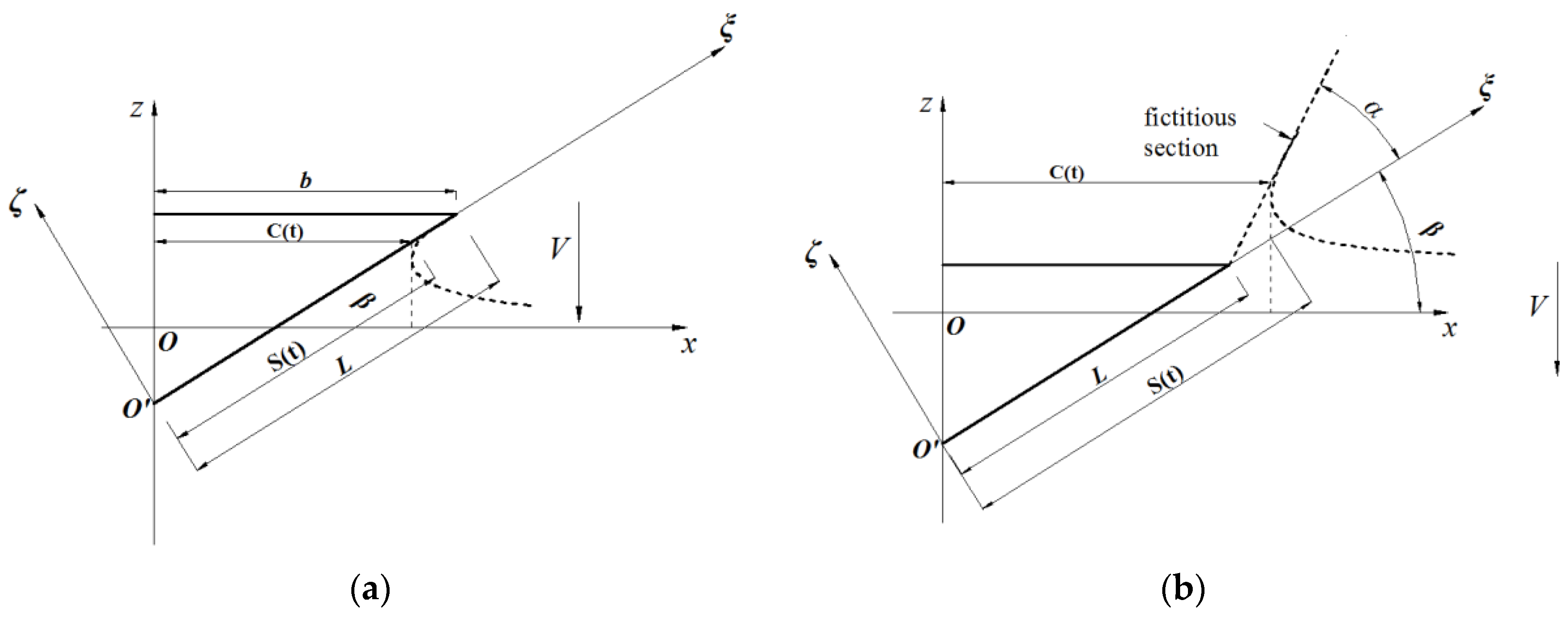
2. Definition of the 2D Water Entry
3. Structural Dynamic Equation
4. Generalized Impact Forces of 2D Sections
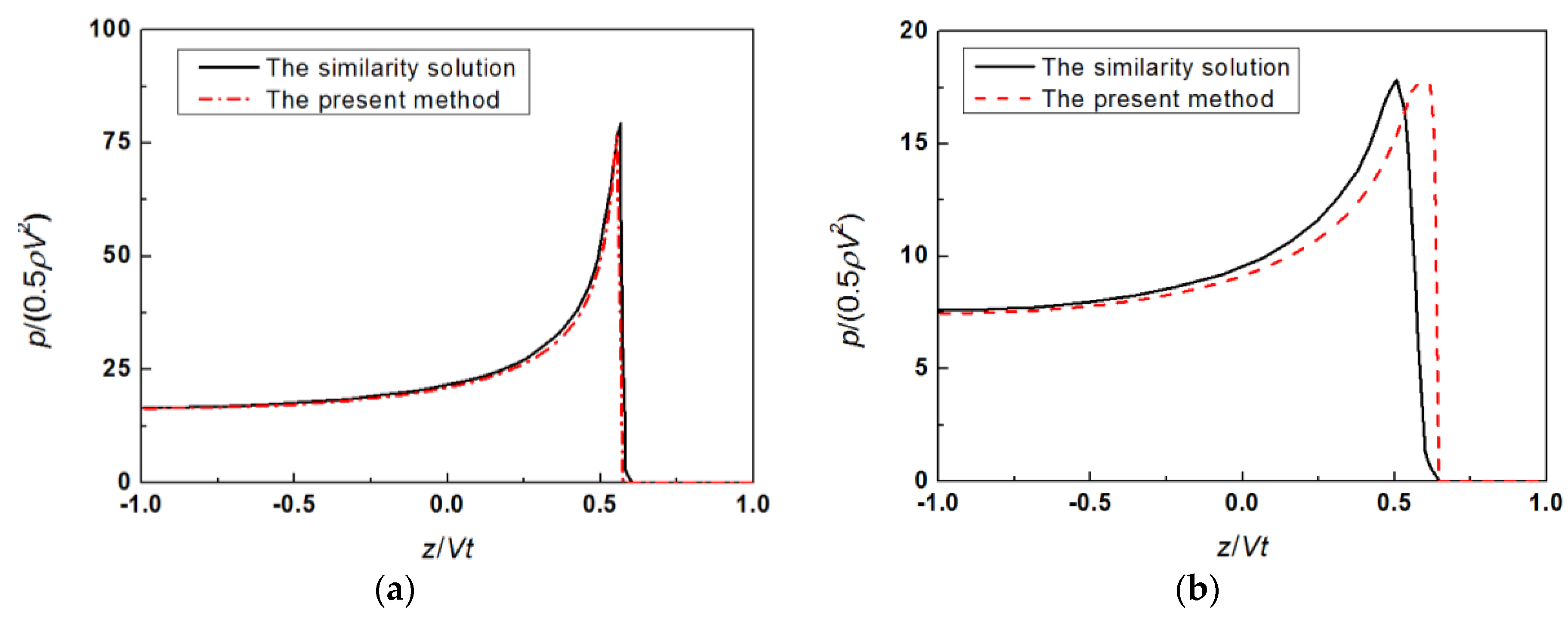
4.1. Generalized Excitation Force
4.2. General Hydrodynamic Coefficients
5. Dynamic Equation of the 3D Wedge
6. Results and Discussions
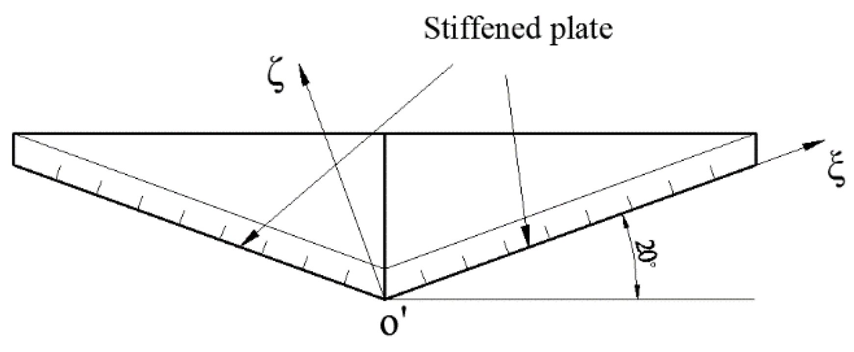
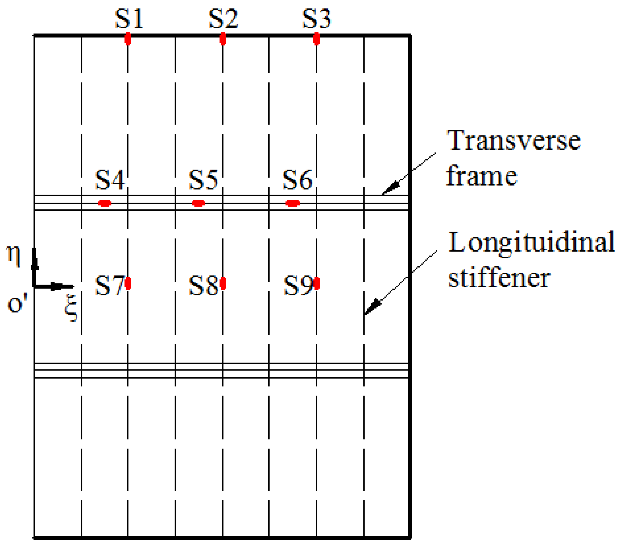
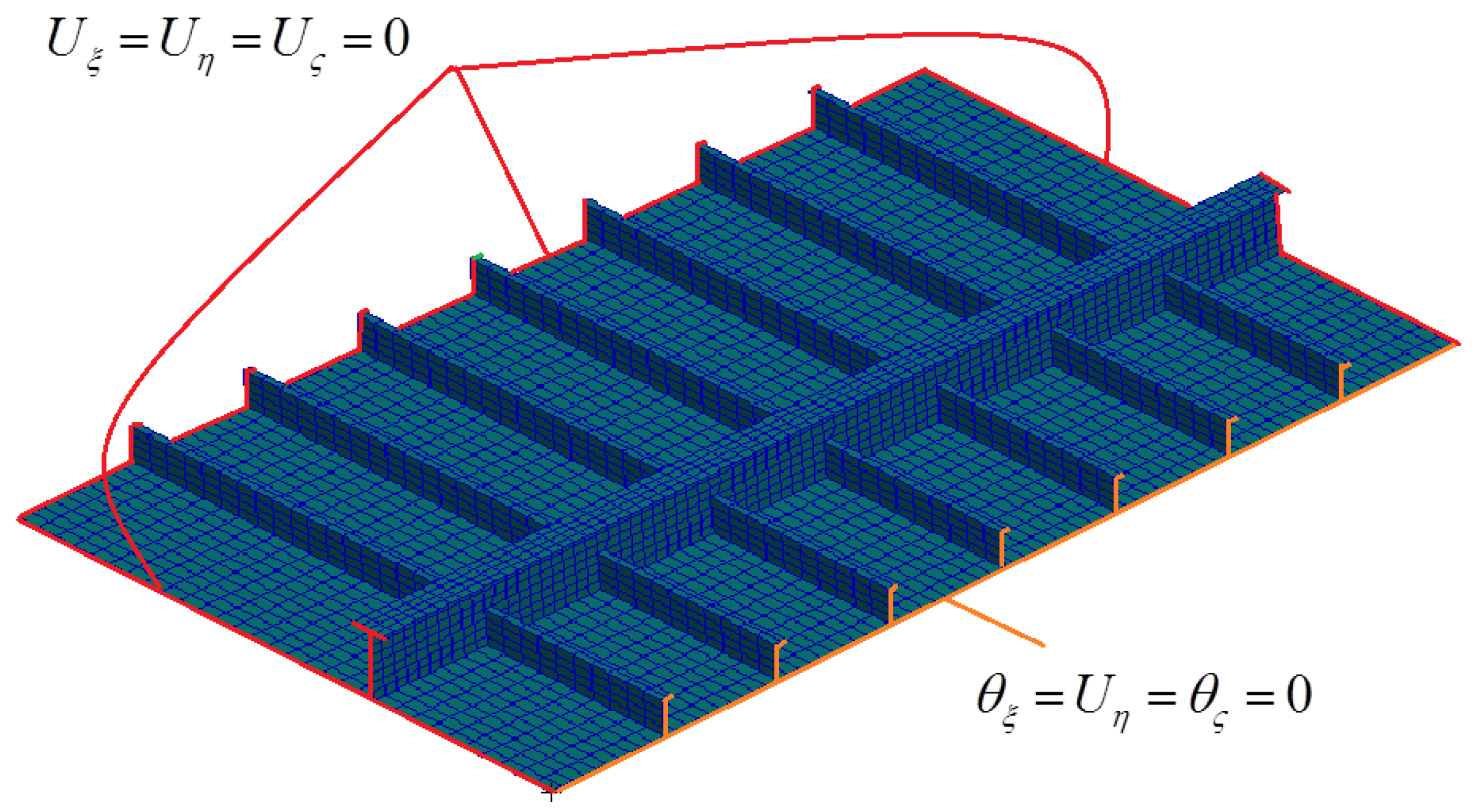
6.1. Description of the Wedge
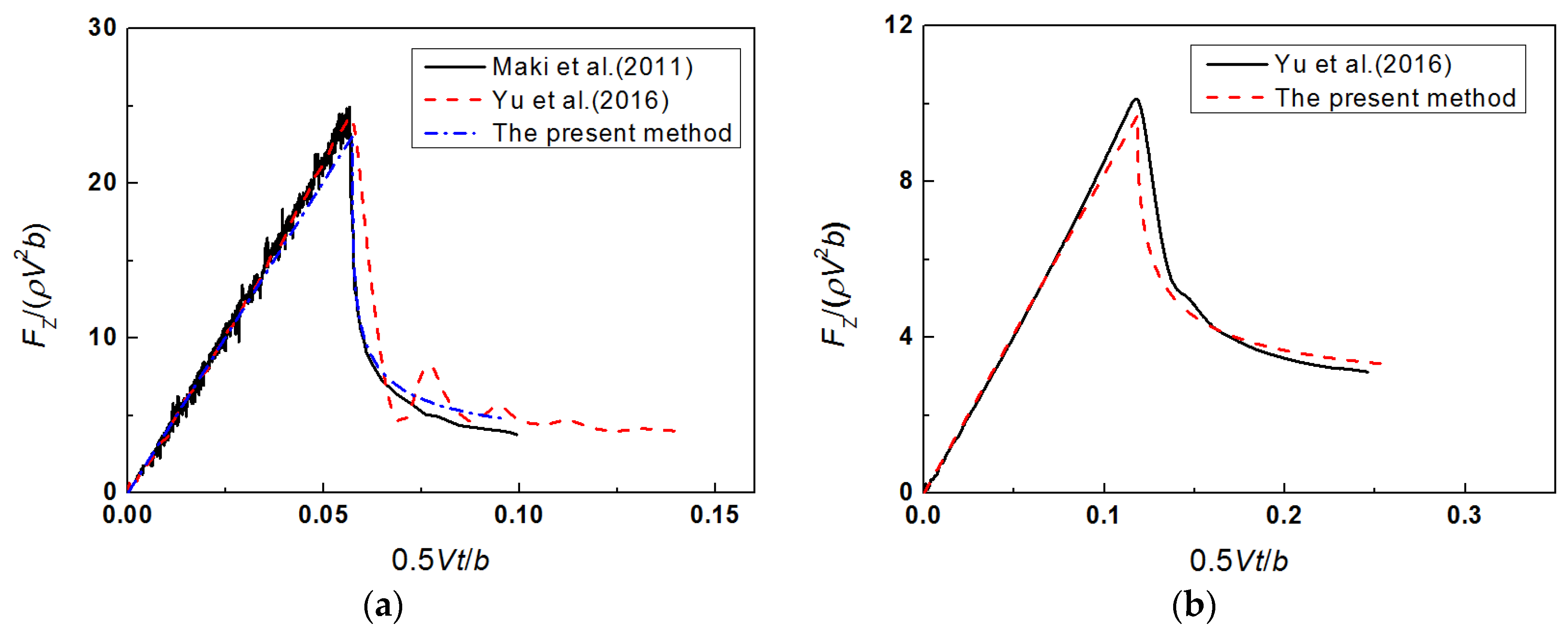
6.2. Validation of the Present Method
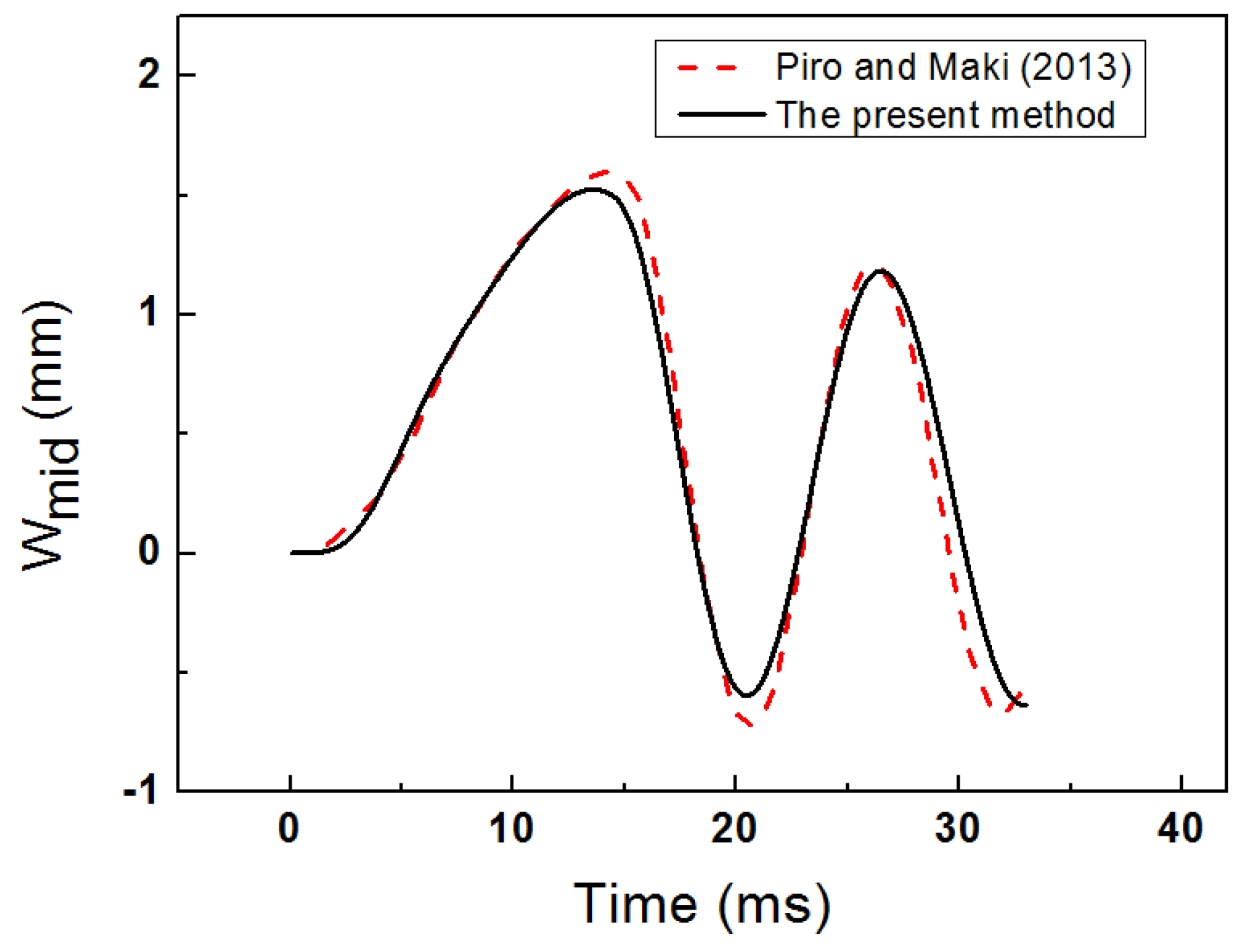
6.2.1. Comparison with Published Literature
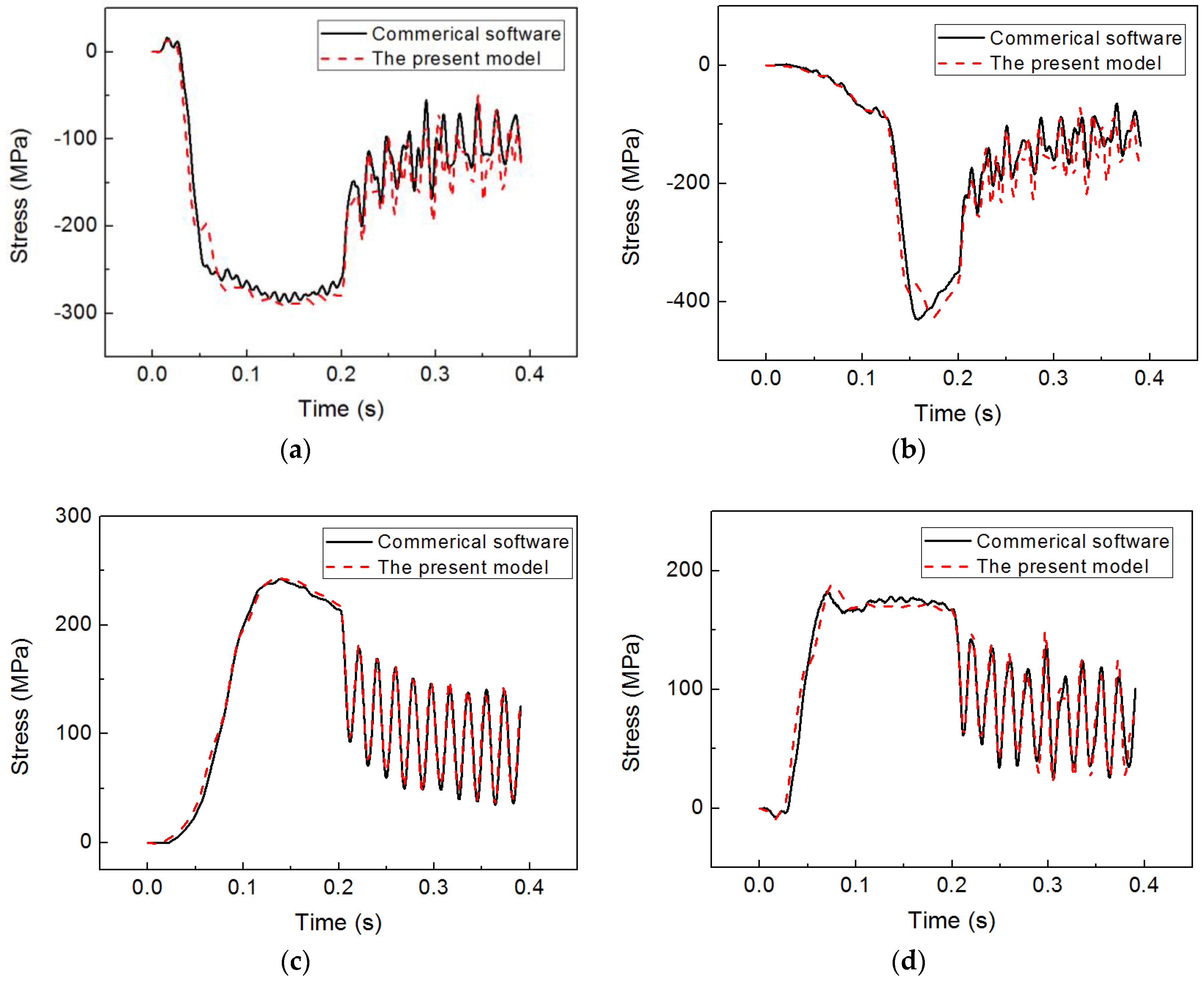
6.2.2. Comparison with the Commercial Software
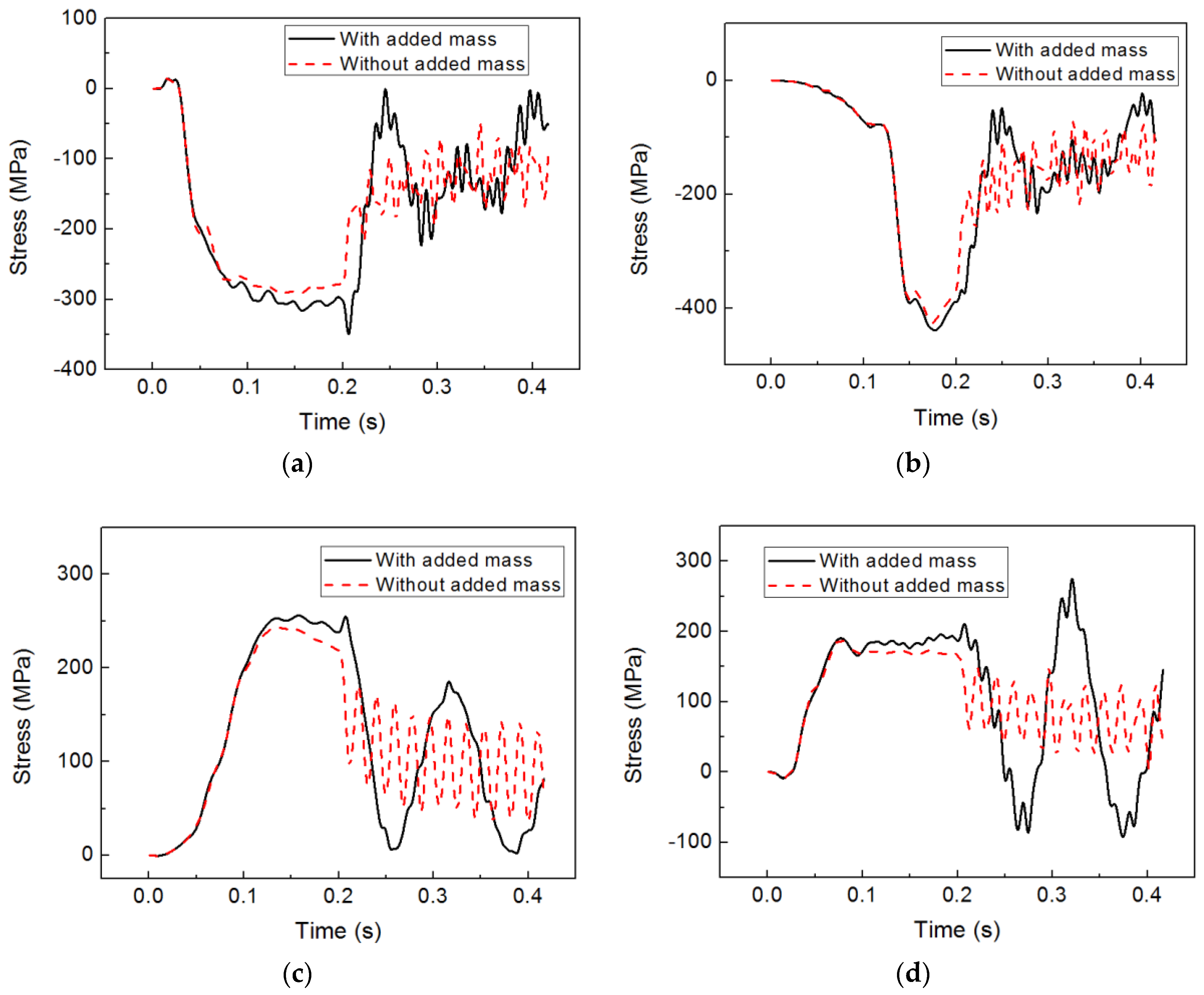
6.3. Effect of the Added Mass
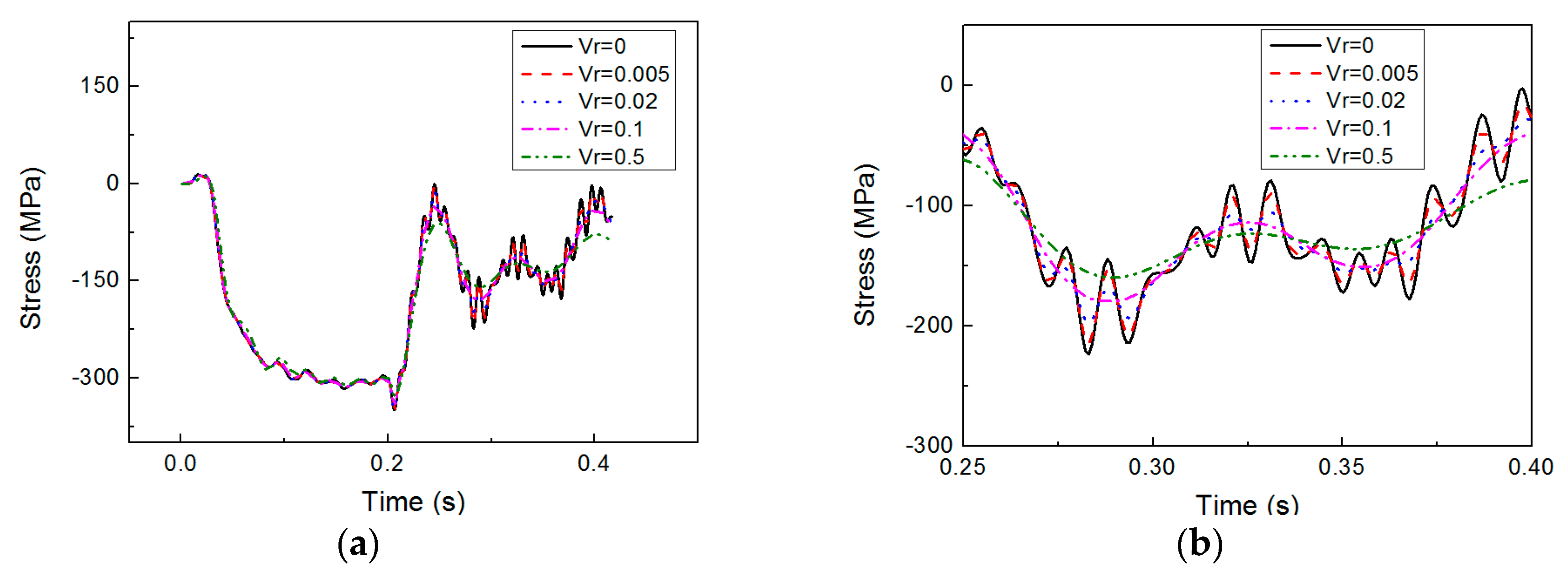
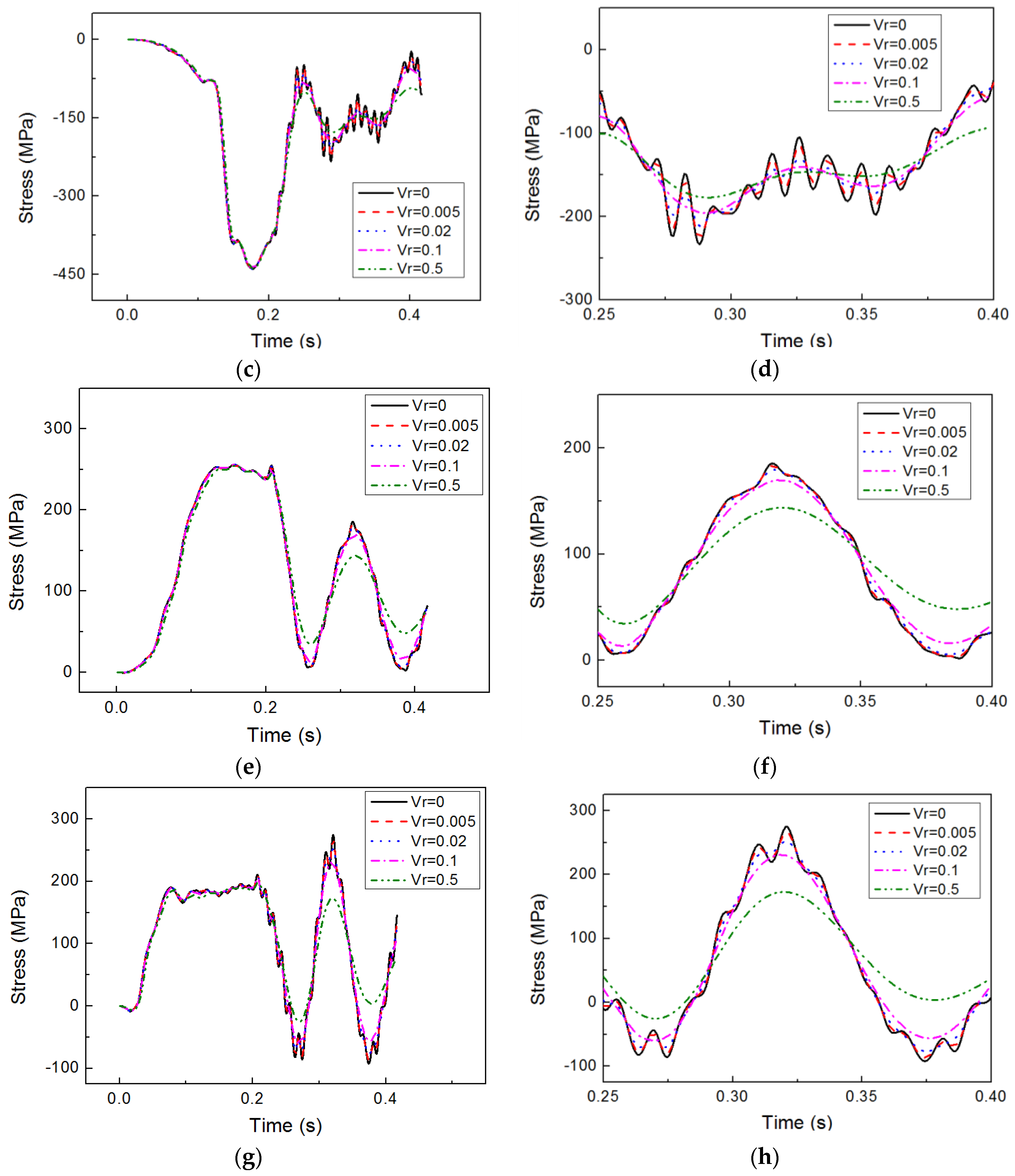
6.4. Effect of the Structural Damping
7. Conclusions
Author Contributions
Acknowledgments
Conflicts of Interest
Appendix A. The Semi-Analytical Model Based on the Modified Logvinovich Model
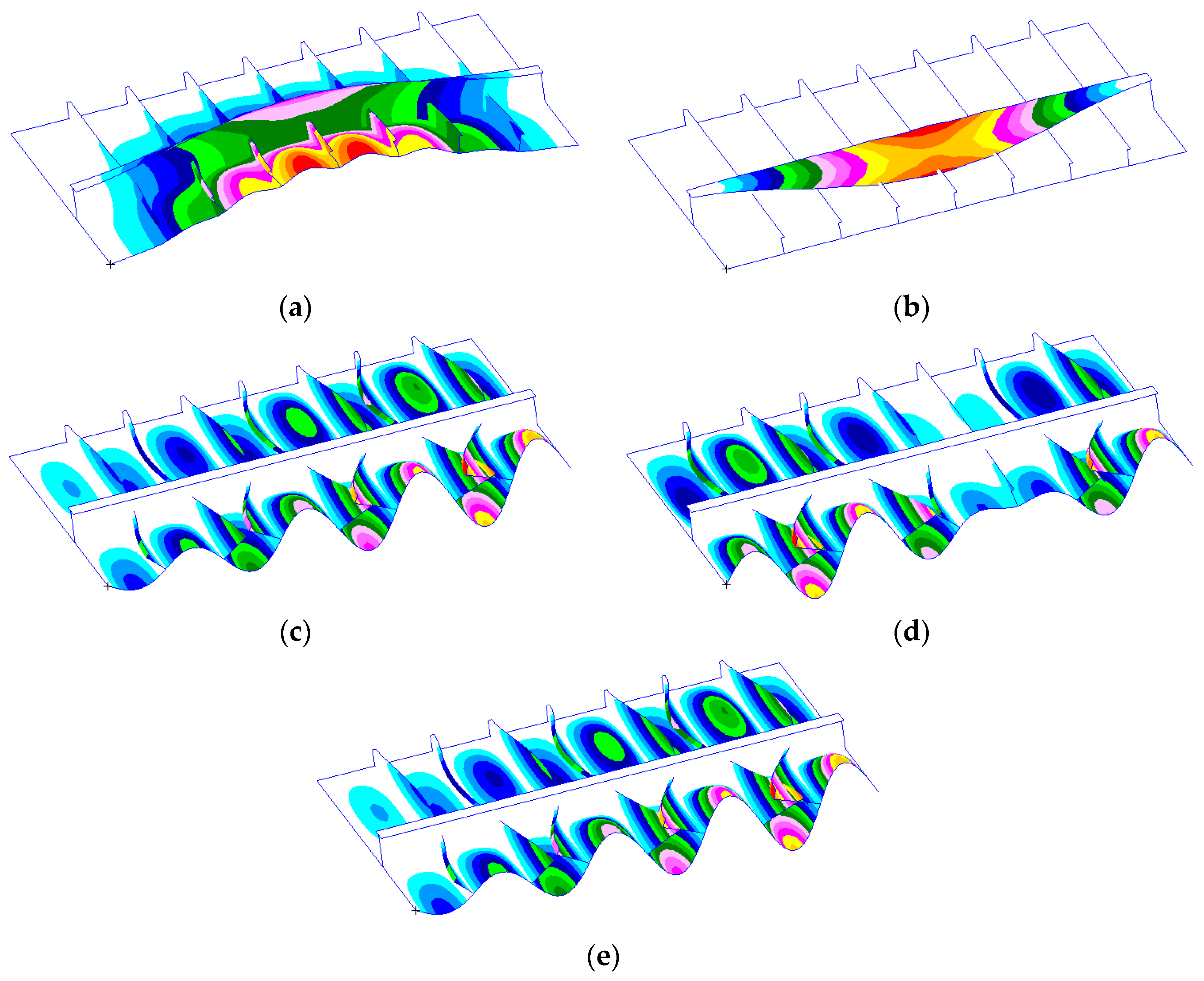
Appendix B. Modal Analysis

| Order | Natural Frequency () | General Mass () | General Stiffness ( × 105) |
|---|---|---|---|
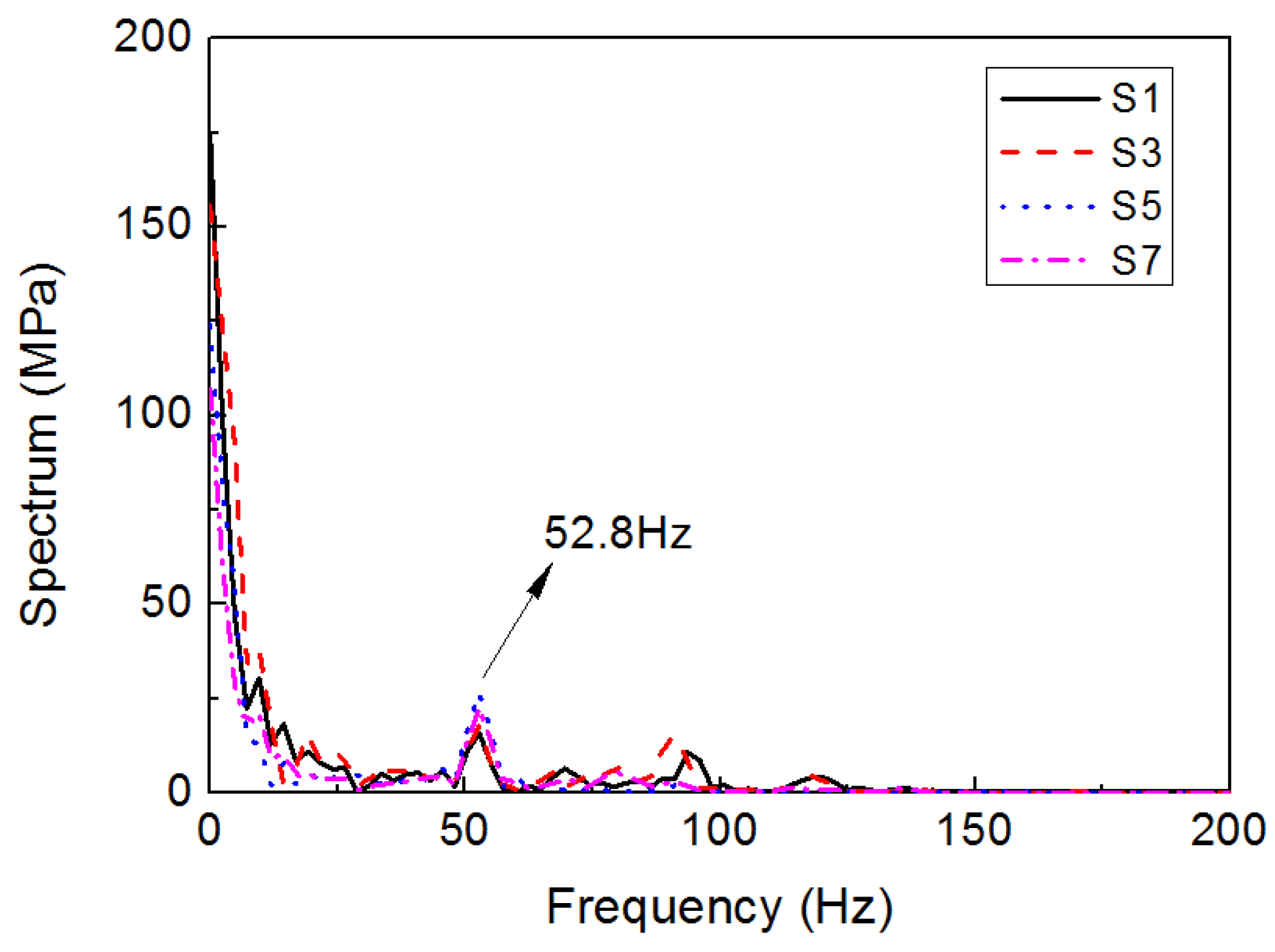
| 1 | 52.89 | 1.00 | 1.10 |
| 2 | 61.18 | 1.00 | 1.48 |
| 3 | 63.89 | 1.00 | 1.61 |
| 4 | 65.69 | 1.00 | 1.70 |
| 5 | 66.32 | 1.00 | 1.74 |


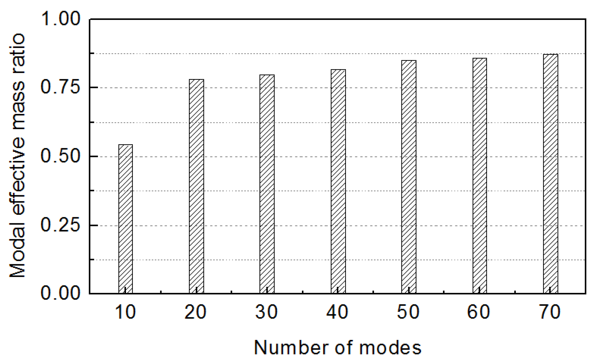
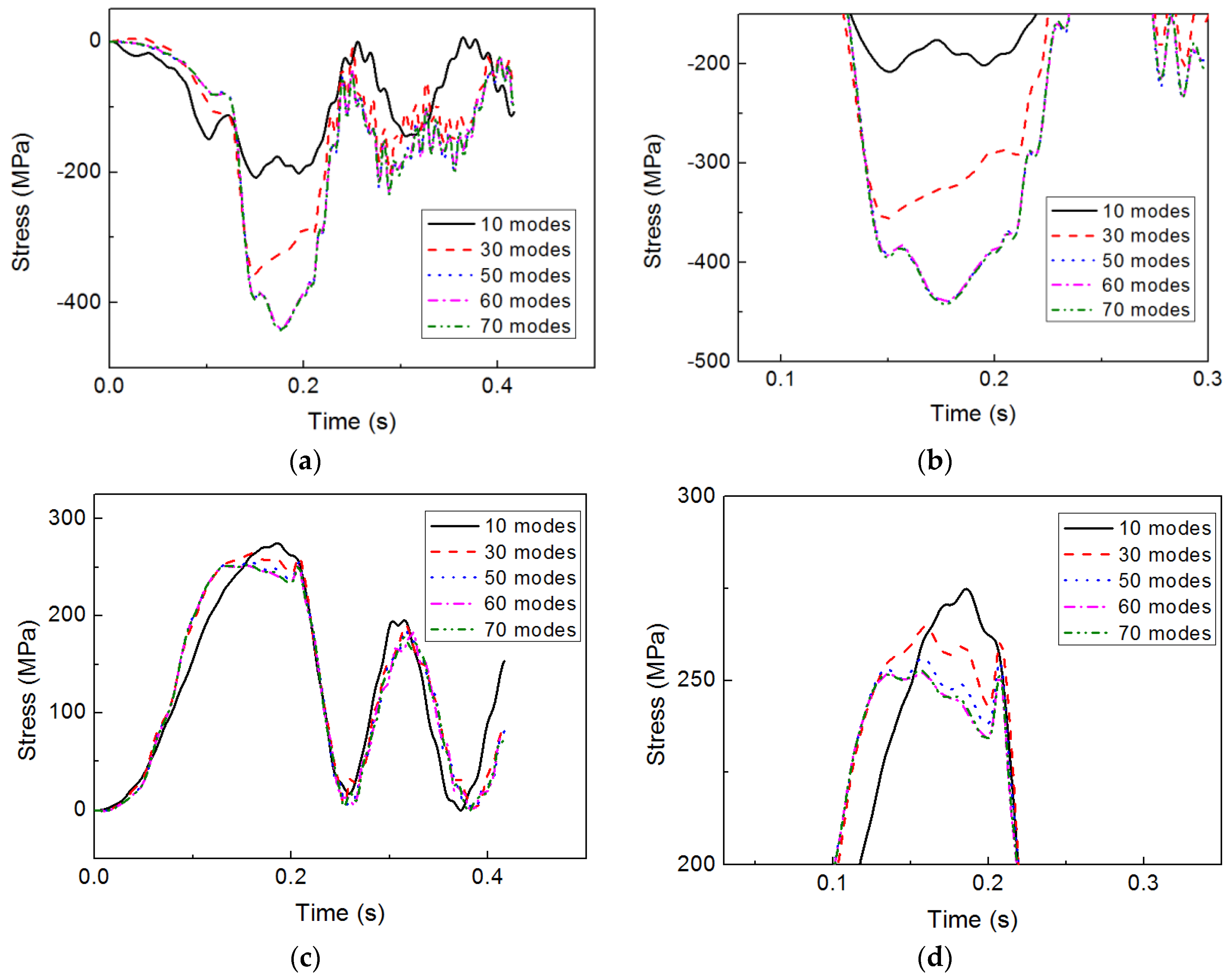
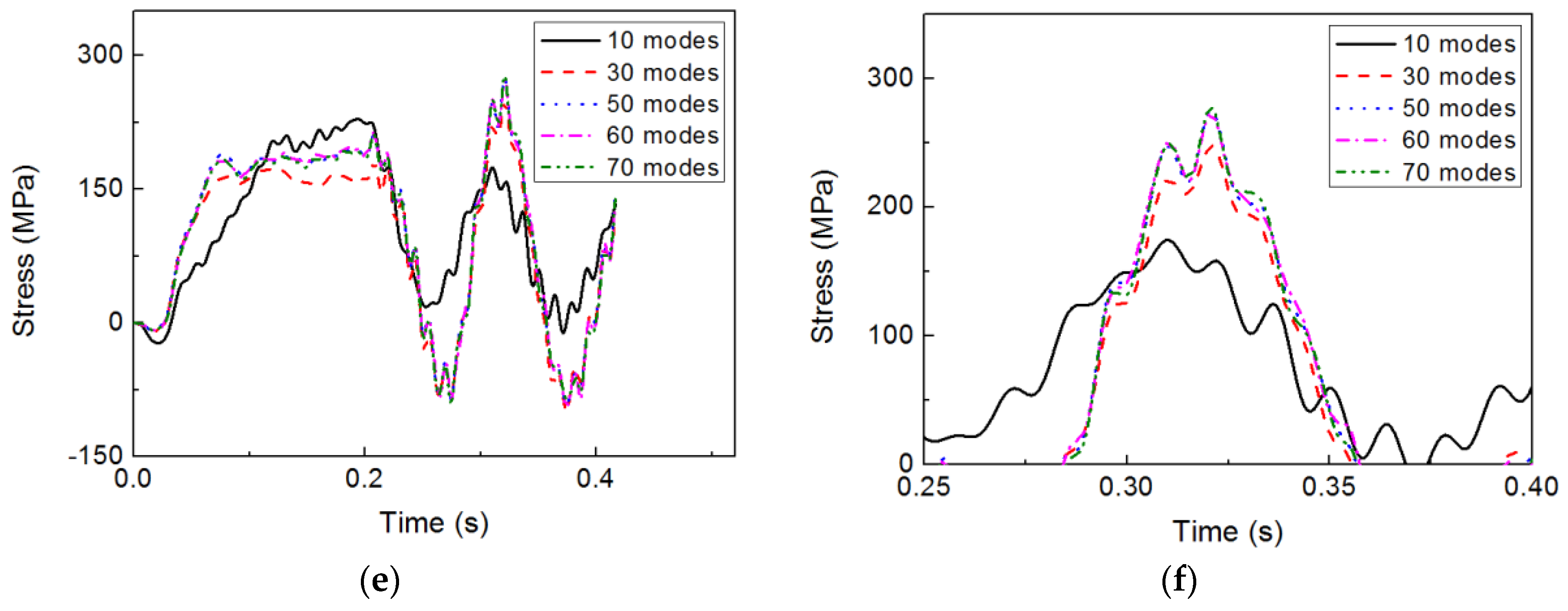
Appendix C. Modal Convergence Study


References
- Xu, G.D.; Duan, W.Y.; Wu, G.X. Numerical simulation of oblique water entry of an asymmetrical wedge. Ocean Eng. 2008, 35, 1597–1603. [Google Scholar] [CrossRef]
- Von Karman, T. The Impact on Seaplane Floats during Landing; Technical Report Archive & Image Library; NTRS: Washington, DC, USA, 1929. [Google Scholar]
- Wagner, H. Uber Stoss- und Gleitvorgange an der Oberflache von Flussigkeiten. ZAMM J. Appl. Math. Mech. 1932, 12, 193–215. [Google Scholar] [CrossRef]
- Zhao, R.; Faltinsen, O. Water entry of two-dimensional bodies. J. Fluid Mech. 1993, 246, 593–612. [Google Scholar] [CrossRef]
- Tassin, A.; Jacques, N.; El Malki Alaoui, A.; Nême, A.; Leblé, B. Assessment and comparison of several analytical models of water impact. Int. J. Multiphys. 2010, 4, 125–140. [Google Scholar] [CrossRef]
- Tassin, A.; Korobkin, A.A.; Cooker, M.J. On analytical models of vertical water entry of a symmetric body with separation and cavity initiation. Appl. Ocean Res. 2014, 48, 33–41. [Google Scholar] [CrossRef]
- Yu, P.Y.; Ren, H.L.; Li, H.; Wang, S.; Sun, L.M. Slamming study of wedge and bow-flared sections. J. Ship Mech. 2016, 20, 1109–1120. [Google Scholar] [CrossRef]
- Wang, J.; Lugni, C.; Faltinsen, O.M. Experimental and numerical investigation of a freefall wedge vertically entering the water surface. Appl. Ocean Res. 2015, 51, 181–203. [Google Scholar] [CrossRef]
- Bao, C.M.; Wu, G.X.; Xu, G. Simulation of freefall water entry of a finite wedge with flow detachment. Appl. Ocean Res. 2017, 65, 262–278. [Google Scholar] [CrossRef]
- Kamath, A.; Bihs, H.; Arntsen, O.A. Study of water impact and entry of a free falling wedge using computational fluid dynamics simulations. J. Offshore Mech. Arct. Eng. 2017, 139. [Google Scholar] [CrossRef]
- Yettou, E.-M.; Desrochers, A.; Champoux, Y. Experimental study on the water impact of a symmetrical wedge. Fluid Dyn. Res. 2006, 38, 47–66. [Google Scholar] [CrossRef]
- Jalalisendi, M.; Shams, A.; Panciroli, R.; Porfiri, M. Experimental reconstruction of 3D hydrodynamic loading in water entry problems through particle image velocimetry. Exp. Fluids 2015, 56, 41. [Google Scholar] [CrossRef]
- Jalalisendi, M.; Porfiri, M. Water entry of compliant slender bodies: Theory and experiments. Int. J. Mech. Sci. 2017. [Google Scholar] [CrossRef]
- Korobkin, A.; Gueret, R.; Malenica, S. Hydroelastic coupling of beam finite element model with Wagner theory of water impact. J. Fluids Struct. 2006, 22, 493–504. [Google Scholar] [CrossRef]
- Qin, Z.; Batra, R.C. Local slamming impact of sandwich composite hulls. Int. J. Solids Struct. 2009, 46, 2011–2035. [Google Scholar] [CrossRef]
- Khabakhpasheva, T.I.; Korobkin, A.A. Elastic wedge impact onto a liquid surface: Wagner’s solution and approximate models. J. Fluids Struct. 2013, 36, 32–49. [Google Scholar] [CrossRef]
- Datta, N.; Siddiqui, M.A. Hydroelastic analysis of axially loaded Timoshenko beams with intermediate end fixities under hydrodynamic slamming loads. Ocean Eng. 2016, 127, 124–134. [Google Scholar] [CrossRef]
- Shams, A.; Porfiri, M. Treatment of hydroelastic impact of flexible wedges. J. Fluids Struct. 2015, 57, 229–246. [Google Scholar] [CrossRef]
- Shams, A.; Zhao, S.; Porfiri, M. Hydroelastic slamming of flexible wedges: Modeling and experiments from water entry to exit. Phys. Fluids 2017, 29. [Google Scholar] [CrossRef]
- Lu, C.H.; He, Y.S.; Wu, J.X. Coupled analysis of nonlinear interaction between fluid and structure during impact. J. Fluids Struct. 2000, 14, 127–146. [Google Scholar] [CrossRef]
- Maki, K.J.; Lee, D.; Troesch, A.W.; Vlahopoulos, N. Hydroelastic impact of a wedge-shaped body. Ocean Eng. 2011, 38, 621–629. [Google Scholar] [CrossRef]
- Piro, D.J.; Maki, K.J. Hydroelastic analysis of bodies that enter and exit water. J. Fluids Struct. 2013, 37, 134–150. [Google Scholar] [CrossRef]
- Panciroli, R. Dynamic Failure of Composite and Sandwich Structures. In Solid Mechanics and Its Applications; Abrate, S., Castanié, B., Rajapakse, Y., Eds.; Springer: Dordrech, The Netherlands, 2013; Volume 192, pp. 1–45. ISBN 978-94-007-5328-0. [Google Scholar]
- Panciroli, R.; Abrate, S.; Minak, G. Dynamic response of flexible wedges entering the water. Compos. Struct. 2013, 99, 163–171. [Google Scholar] [CrossRef]
- Das, K.; Batra, R.C. Local water slamming impact on sandwich composite hulls. J. Fluids Struct. 2011, 27, 523–551. [Google Scholar] [CrossRef]
- Stenius, I.; Rosén, A.; Kuttenkeuler, J. Hydroelastic interaction in panel-water impacts of high-speed craft. Ocean Eng. 2011, 38, 371–381. [Google Scholar] [CrossRef]
- Faltinsen, O.M. Water entry of a wedge by hydroelastic orthotropic plate theory. J. Ship Res. 1999, 43, 180–193. [Google Scholar]
- Luo, H.; Wang, H.; Guedes Soares, C. Numerical and experimental study of hydrodynamic impact and elastic response of one free-drop wedge with stiffened panels. Ocean Eng. 2012, 40, 1–14. [Google Scholar] [CrossRef]
- Luo, H.; Wang, H.; Guedes Soares, C. Comparative study of hydroelastic impact for one free-drop wedge with stiffened panels by experimental and explicit finite element methods. In Proceedings of the ASME 2011 30th International Conference on Ocean, Offshore and Arctic Engineering, Rotterdam, The Netherlands, 19–24 June 2011. [Google Scholar] [CrossRef]
- China Classification Society (CCS). Rules for Construction and Classification of Sea-Going High Speed Craft; China Classification Society: Beijing, China, 2012; pp. 50–57. [Google Scholar]
- Wu, M.; Moan, T. Sensitivity of extreme hydroelastic load effects to changes in ship hull stiffness and structural damping. Ocean Eng. 2007, 34, 1745–1756. [Google Scholar] [CrossRef]
- Korobkin, A. Analytical models of water impact. Eur. J. Appl. Math. 2004, 15, 821–838. [Google Scholar] [CrossRef]


| Particulars | Value | Unit | |
|---|---|---|---|
| Density | 7850 | kg/m3 | |
| Modulus of elasticity | 2.07 × 10¹¹ | pa | |
| Poisson ratio | 0.3 | - | |
| Thickness of the plate | 12 | mm | |
| Distance between longitudinal stiffeners | 675 | mm | |
| Dimensions of longitudinal stiffeners | tw | 9 | mm |
| hw | 200 | mm | |
| tf | 19.7 | mm | |
| bf | 39.8 | mm | |
| Distance between transverse frames | 2400 | mm | |
| Dimensions of transverse frames | tw | 10 | mm |
| hw | 400 | mm | |
| tf | 16 | mm | |
| bf | 200 | mm | |
| Positions | σwe (MPa) | σwoe (MPa) | σwe/σwoe-1 |
|---|---|---|---|
| S1 | 349.12 | 290.94 | 20.00% |
| S2 | 464.76 | 446.3 | 4.14% |
| S3 | 439.55 | 426.27 | 3.12% |
| S4 | 74.184 | 72.59 | 2.20% |
| S5 | 256.11 | 242.95 | 5.42% |
| S6 | 193.54 | 185.86 | 4.13% |
| S7 | 274.3 | 188.18 | 45.76% |
| S8 | 285.48 | 273.12 | 4.53% |
| S9 | 282.5 | 267.11 | 5.76% |
© 2018 by the authors. Licensee MDPI, Basel, Switzerland. This article is an open access article distributed under the terms and conditions of the Creative Commons Attribution (CC BY) license (http://creativecommons.org/licenses/by/4.0/).
Share and Cite
Yu, P.; Ong, M.C.; Li, H. Effects of Added Mass and Structural Damping on Dynamic Responses of a 3D Wedge Impacting on Water. Appl. Sci. 2018, 8, 802. https://doi.org/10.3390/app8050802
Yu P, Ong MC, Li H. Effects of Added Mass and Structural Damping on Dynamic Responses of a 3D Wedge Impacting on Water. Applied Sciences. 2018; 8(5):802. https://doi.org/10.3390/app8050802
Chicago/Turabian StyleYu, Pengyao, Muk Chen Ong, and Hui Li. 2018. "Effects of Added Mass and Structural Damping on Dynamic Responses of a 3D Wedge Impacting on Water" Applied Sciences 8, no. 5: 802. https://doi.org/10.3390/app8050802
APA StyleYu, P., Ong, M. C., & Li, H. (2018). Effects of Added Mass and Structural Damping on Dynamic Responses of a 3D Wedge Impacting on Water. Applied Sciences, 8(5), 802. https://doi.org/10.3390/app8050802