Abstract
It is critical to detect hidden, periodically impulsive signatures caused by tooth defects in a gearbox. A hybrid demodulation method for detecting tooth defects has been developed in this work based on the variational mode decomposition algorithm combined with modulation intensity distribution. An original multi-component signal is first non-recursively decomposed into a number of band-limited mono-components with specific sparsity properties in the spectral domain using variational mode decomposition. The hidden meaningful cyclostationary features can be clearly identified in the bi-frequency domain via the modulation intensity distribution (MID) technique. Moreover, the reduced frequency aliasing effect of variational mode decomposition is evaluated as well, which is very useful for separating noise and harmonic components in the original signal. The influences of the spectral coherence density and the spectral correlation density of the modulation intensity distribution on the demodulation were also investigated. The effectiveness and noise robustness of the proposed method have been well-verified using a simulated signal compared with the empirical mode decomposition algorithm associated with modulation intensity distribution. The proposed technique is then applied to detect four different defects in a multi-stage gearbox. The results demonstrated that the demodulated numerical information and pigmentation directly illustrated in the bi-frequency plot of the modulation intensity distribution can be successfully used to quantitatively differentiate the four gear defects.
1. Introduction
Gearbox fault detection is significant for the security and reliability of mechanical equipment [1]. Faults caused by gear failures account for 10% of the malfunctions in rotating machines and 80% of those in mechanical transmission systems [2]. Therefore, it is necessary to effectively detect faults in a gearbox in order to prevent accidents and guarantee its efficient operation [3].
Model-based methods in dynamic systems have been continuously proposed for gear fault diagnosis [4,5,6]. Nowadays, vibration-based analysis approaches are widely used to identify tooth faults due to their effectiveness and ease of measurement [2]. However, the collected vibration signals of a multi-stage gearbox have strong modulation signatures [7,8] due to the existence of meshing frequencies, multi-harmonics, and coupled frequencies generated by modulation. Thus, in order to extract important signatures from raw vibration signals, various signal processing techniques have been utilized in gear defect detection, such as wavelet packet transform (WPT) [9] and empirical mode decomposition (EMD) [10]. Nevertheless, WPT alone is not suitable for fault diagnosis in a multi-stage gearbox because many close or identical frequency components occur in the signals [9]. In addition, EMD is an adaptive signal decomposition approach and has been extensively used to decompose a multi-component signal into several sub-signals, but it still has a major drawback of mode mixing [11].
Recently, variational mode decomposition (VMD) has been pioneered by Dragonmiretskiy and Zosso [12,13], which is a non-recursive signal processing technique with a firm theoretical foundation compared with EMD. Meanwhile, the performances of VMD on non-stationary signal analysis have been also evaluated and compared with other adaptive signal processing methods. For instance, the equivalent filter bank property of the VMD has been explored, and the results demonstrated that VMD can be considered as a WPT or a generalized short time Fourier transform (STFT) with a varying window width [14]. Moreover, it has been demonstrated that VMD can better extract the bearing fault signatures of acoustic signals in comparison with EMD [15]. A hybrid defect detecting technique has been also proposed for denoising and non-stationary signature extraction, which joins VMD and the majoriation–minization-based total variation denoising (TV-MM) technique [16]. Because of these merits of VMD, it has been well-utilized for detecting rubbing faults in a rotor system [13]. However, VMD still has some limitations regarding signal demodulation analysis. For example, VMD cannot directly identify the numerical value of demodulated signatures. Moreover, results using the above-mentioned signal decomposition methods alone are usually unsatisfactory for detecting tooth defects, especially in a multistage gearbox.
Demodulation analysis is also a popular technique for detecting defects in rotating machines [17]. Some new works on demodulation analysis for fault diagnosis in bearings and gears have been developed; for example, a modulation signal bispectrum (MSB) and the modulation signal bispectrum-based sideband estimator (MSB-SE) method [18,19]. One advantage of some demodulation techniques is that the numerical modulated information can be directly detected in the time domain [20] or via power spectral density in the spectral domain [21]. Furthermore, complex demodulated signals can be investigated using joint time-frequency or time-scale analysis techniques [22], but the meaning of the time-frequency plot is still hard to identify for non-experts. Consequently, the cyclostationary method seems to be a promising technique to identify periodic modulation components [23], which is very effective when the analyzed signal contains various components for complex machinery [24]. Modulation intensity distribution (MID) is regarded as a generalization of the spectral correlation density and can be applied to demodulation analysis of a cyclostationary signal [17]. MID can detect the modulation components in a first-order modulation signal, but it still cannot accurately detect the carrier components and the corresponding modulation components in a multi-harmonic modulated vibration signal.
Therefore, a hybrid demodulation approach has been proposed for fault diagnosis in a multi-stage gearbox in this work, which combines the VMD and MID techniques and has some complementary advantages in the demodulation of a complex signal. This article is organized as follows: the VMD theory and its reduced frequency aliasing effects are introduced in Section 2. The hybrid demodulation technique is proposed in Section 3. Its effectiveness is first demonstrated using a simulated signal combined with MID associated with the EMD technique. The proposed approach is then applied to detect four types of tooth fault in a multi-stage gearbox in Section 4. Finally, conclusions are drawn in Section 5.
2. Theory of VMD
2.1. A Brief Introduction of the VMD Algorithm
VMD can decompose a signal into a number of band-limited intrinsic mode functions (BLIMFs) that have the sparsity property in their nature [12,25], which can be represented as follows:
where denotes the Dirac delta function, = −1, denotes the norm, is the derivative with respect to , denotes the convolution operator, and is the center frequency. A solution of the minimization Equation (1) can be defined as a saddle point of the augmented Lagrangian that is given below:
in which denotes the balancing parameter of the data-fidelity constraint. The benefits of the embedded Wiener filtering in the algorithm are that VMD is much more robust to sampling and noise. The mode and the center frequency are both iteratively updated in the frequency domain. Consequently, the temporal mode is obtained as the real part of the inverse Fourier transform of the filtered analytic signal using the determined center frequency and bandwidth.
The VMD algorithm in detail can be found in [12,13]. The whole process of the VMD algorithm is shown in Figure 1. The behavior of VMD in the presence of irregular samples, an impulsive response, fractional Gaussian noise, and tone separation has been thoroughly investigated in [14]. Mode aliasing is associated with tone separation to some extent and will be illustrated in the following subsection.
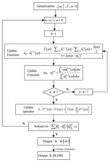
Figure 1.
The flow charts of variational mode decomposition (VMD).
2.2. Reduced Frequency Aliasing Effect
Mode aliasing or mode mixing is a common phenomenon in the process of EMD, which is defined as signal components in the same intrinsic mode function (IMF) mode containing different disparate scales or components in the same scale residing in different IMF components [26]. Actually, mode aliasing will affect the feature extraction seriously. In order to verify a reduction in the effects of frequency aliasing of VMD, a multi-harmonic signal is analyzed in this subsection. The multi-harmonic signal can be written as follows:
The sampling frequency of is 2000 Hz, while the number of sampling points N is 2000. The temporal waveform of the simulated signal and its Fast Fourier Transform (FFT) spectrum are both shown in Figure 2. Obviously, there are five frequency components, namely 30, 150, 200, 300, and 500 Hz, in the spectrum.
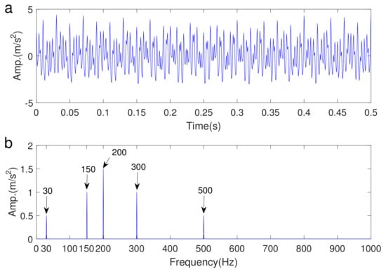
Figure 2.
The simulated multi-harmonic signal: (a) temporal waveform (b) its Fast Fourier Transform (FFT) spectrum.
When the simulated signal was decomposed with VMD, the number of modes K was set to 5, and two kinds of initialization of the center frequency , denoted as and , were adopted in the verification, respectively. Finally, five BLIMFs achieved with VMD and their corresponding spectra are illustrated in Figure 3a–d, respectively. It can be seen in Figure 3a,b that all of the components in the signal can be separated very well without any redundant components and mode mixing when was initialized by . All five components of the original signal can be also detected successfully in Figure 3c,d when the initialization of was chosen as in conjunction with a small value of . Meanwhile, the IMF components obtained by EMD and their spectra are given in Figure 3e,f. However, it is found that there is no ideal harmonic component in Figure 3e because of the severe mode aliasing of EMD. In addition, it should be noted that the decomposed BLIMFs are very different from the IMFs shown in Figure 3f, since VMD is no longer a recursive decomposition algorithm.
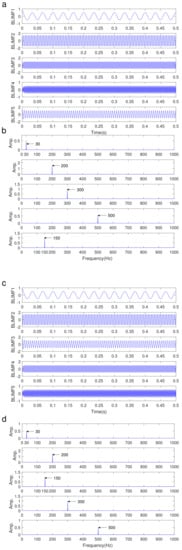
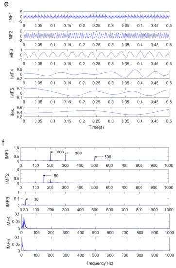
Figure 3.
Multi-harmonic signal analysis: (a) results of VMD with the initialization of the center frequency and their spectra (b); (c) results of VMD with the initialization of the center frequency and their spectra (d); (e) results of empirical mode decomposition (EMD) and their spectra (f). IMF = intrinsic mode function; BLIMF = band-limited intrinsic mode function.
3. The Proposed Hybrid Demodulation Technique
3.1. Modulation Intensity Distribution
MID is a kind of signal demodulation method that has cyclostationary properties. It is very suitable for the analysis of first-order modulation (discrete carrier frequency) and is also applicable to the analysis of a two-order modulation (random carrier frequency) signal [20]. MID can reveal the relationship between the cyclic frequency and carrier frequency in the bi-frequency domain. In order to better interpret the principle of MID, a simple modulated signal can be assumed as below:
where is the amplitude, , and is frequency doubling. The spectrum of the above signal consists of a spectrum line located at the center frequency (carrier signal) together with some spectrum lines symmetrically located around the frequency and spaced by cyclic frequency (modulation components) in Figure 4.
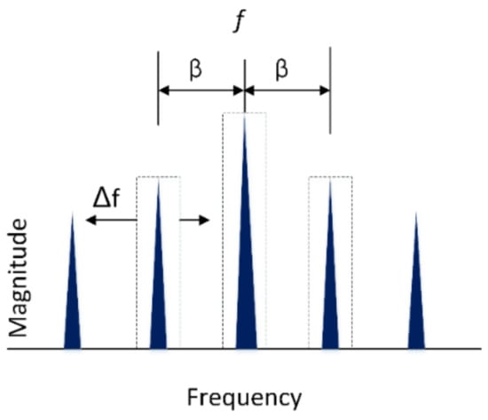
Figure 4.
The process of the sideband filtering.
Actually, the core ideal of MID is the sideband filter that allows us to extract the potential carrier signal together with the corresponding modulating signals. Thus, the filtered signal by this technique only has specific signal components and reduced noise. The filtered signal can be given by [27]
where represents the filtered version of in a narrow frequency band The result of the proposed sideband filtering might be then utilized for computing the relationship between three spectral components spaced by the frequency that is indicated in the presence of modulation [11]. The spectral correlation (SCor) density can be used as an indicator to detect modulation components in the signal. SCor density is defined by
where is the completed envelope of the filtered version of the signal in a narrow frequency band can be calculated as an STFT with a rectangular time window [28].
As is given in Equation (8), the relationship between and is
Therefore, Equation (6) may be written as a time average of a cyclic periodogram.
Then, SCor density can be represented as follows:
where is defined by Equation (5). It should be noted that multiplication by in Equation (9) performs a frequency shifting operation by cyclic frequency so as to offer the same central frequency for components and . In addition, since the operation proposed in Equation (7) can be illustrated as a joint down-sampling and filtering procedure, the down-conversion operation takes place during the computation of . Based on Equation (10), the spectral correlation density between components and is given by
Similarly, the SCor density can be also computed between components and , that is,
It should be noted that frequency shifting in Equations (11) and (12) causes the frequency to be the center frequency for both filtered components. To find the relationship between three spectral components spaced by cyclic frequency , the two SCor densities introduced in Equations (11) and (12) are adopted to calculate the MID using a given which can be expressed by
Practically, the product of SCor densities as the MID might not be the most utilized metric because of large differences in signal energy in lots of frequency bands. In such cases, the illustration of MID maps may be much more useful when the absolute measure of modulation intensity is normalized between 0 and 1. Therefore, the can be readily extended to the use of the spectral coherence (SCoh) density as the MID [16]. SCoh density is given by
Then, the expression of MID with SCoh is also given below:
Certainly, both and can be employed in signal demodulation. The difference between them will be investigated in the following subsection.
3.2. A Hybrid Demodulation Technique via MID and VMD
Since the acquired vibration signals of a rotating machine are usually multi-components and complex modulation signals, VMD can be used as a pre-processing method to decompose a complex signal into a series of mono-harmonic components so as to further improve the demodulation performance of the MID. Thus, the developed hybrid demodulation technique has complementary merits in the demodulation of a complex signal, whose effectiveness will be first demonstrated using a simulated signal.
A numerical signal is simulated with an impulsive signal , a multi-harmonic signal and Gaussian white noise , which is written by [29]
where the impulsive signal and the multi-harmonic signal are separately given by
The sampling frequency and number of sampling points of the signal in Equation (17) are set to 40,960 Hz and 4096, respectively. The carrier frequency of the impulsive component is 3000 Hz in Equation (18). The damping period of is T = 0.01 s, so its modulation frequency is 100 Hz. Two noise variances of the simulated signal are considered in order to verify the noise robustness of the proposed technique. The original temporal waveform of the simulated signal and its spectrum are shown in Figure 5. It can be seen in Figure 5a that the simulated impulsive signal is almost buried in the multi-harmonic signal by the added noise. MID is then used with the meaningful BLIMF2 for the demodulation.
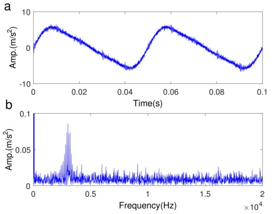
Figure 5.
Simulated vibration signal (a) the time domain waveform (b) the FFT spectrum.
The impulsive components usually represent transient signatures generated by a local defect in a rotating machine. Sub-band components of the simulated signal are obtained by the VMD and EMD techniques, which are found in Figure 6a,b, respectively. VMD can not only effectively detect the impulsive signatures (see BLIMF2 in in Figure 6a), but also successfully identify the multi-harmonic component (see BLIMF1 in Figure 6a). However, EMD can only detect the impulsive signal (IMF3 in Figure 6b).
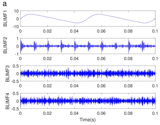
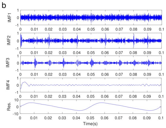
Figure 6.
The decomposed BLIMFs of the simulated vibration signal using VMD (a) and IMF3 using EMD (b).
is then used to analyze the raw simulated signal, and the result is shown in Figure 7. We can find that the cyclic frequency and the carrier frequency cannot be obviously detected due to the added strong noise as well as the influences of the multi-harmonic components. Since the impulsive signal has been successfully identified with VMD, MID is then used to demodulate the meaningful BLIMF2. of the BLIMF2 is shown in Figure 8a, where it can be found that the carrier frequency is 3000 Hz and the cycle frequency (modulation frequency) as well as its multipliers are about 100 Hz. The validation of the proposed hybrid technique is thus well-demonstrated. Moreover, MID is also used to analyze the IMF3 achieved by EMD. of the IMF3 is illustrated in Figure 8b. It can be clearly seen in Figure 8a,b that the result of the BLIMF2 is much better than that of IMF3.
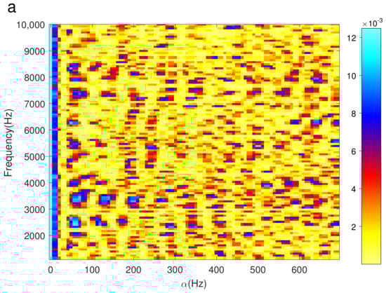
Figure 7.
The of the original simulated vibration signal (the noise variance is 0.3).
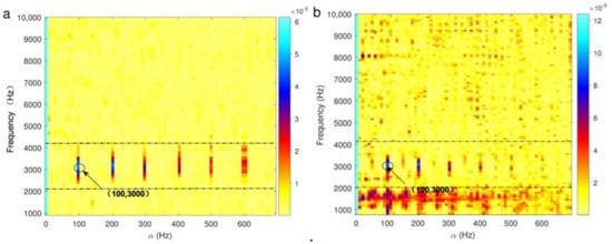
Figure 8.
The of the decomposed BLIMF2 using VMD (a) and IMF3 using EMD (b).
A noise variance of 0.7 is set in the simulated signal in Figure 9. is then used to analyze the simulated signal, and the result is found in Figure 7a. We can find that the cyclic frequency and the carrier frequency cannot be obviously detected due to the strong noise. Once more, MID is also used to demodulate the BLIMF2 component. of the BLIMF2 is shown in Figure 9b, where it can be clearly seen that the carrier frequency is 3000 Hz and the cycle frequency (modulation frequency) is about 100 Hz. This demonstrates the noise robustness of the proposed technique.
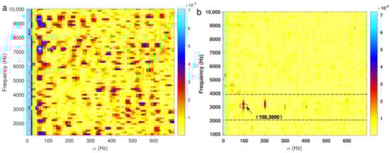
Figure 9.
The of the simulated vibration signal (the noise variance is 0.7) (a) and the decomposed BLIMF2 using VMD (b).
In addition, we will also investigate the difference in the and algorithms in signal demodulation. Thus, the algorithm is also used to analyze the BLIMF2 component and the IMF3 component, respectively. It can be found in Figure 10a,b that the carrier frequency and the cycle frequency are both detected, but the multipliers of the cycle frequencies are not very clearly detected compared with Figure 8a,b. The reason is that the spectral correlation indicator cannot fully play the role of a modulation intensity factor. Thus, spectral coherence analysis will be used in the MID in the following application. The effectiveness of the proposed hybrid demodulation technique will be further investigated using practical gear vibration signals.
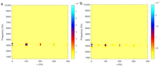
Figure 10.
The of the decomposed BLIMF2 using VMD (a) and IMF3 using EMD (b).
4. Identification of a Tooth Defect Using the Proposed Technique
A wind turbine is a high-cost and relatively complex system. Malfunctions of gear often occur in wind turbines due to the harsh working conditions [30,31]. The proposed hybrid method of MID combined with VMD is applied to identify four types of tooth faults in a multi-stage gearbox in the Wind Turbine Diagnostics Simulator (WTDS) platform.
4.1. The Test Rig
The WTDS test rig is illustrated in Figure 11a, while a schematic of the testing gearbox is shown in Figure 11b. The power drivetrain system consists of a two-stage parallel gearbox and a two-level epicyclic gearbox. The system was driven by a 3HP motor. The rotating frequency of the input shaft was set to 29.8 Hz, while the sampling frequency was set to 2.56 kHz. The meshing frequency was about 864 Hz. The rotation speed was 3450 r/min. The torque was 6.089 Nm. The parallel gearbox was selected as the test object in this experimental validation, and its structure and specifications are shown in Figure 12a in detail. A VibraQuest data acquisition system was used to collect raw vibration data with piezoelectric acceleration sensors installed on bearing covers of the input shaft and the output shaft in the parallel gearbox. Four types of tooth defect, namely, root crack, chipped tooth, surface fault, and missing tooth, are used in this experiment, which are respectively illustrated in Figure 12b–e.
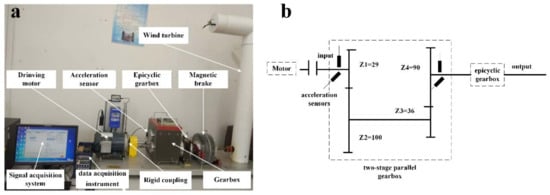
Figure 11.
The Wind Turbine Diagnostics Simulator (WTDS) experimental setup (a) schematic of the testing gearbox (b).
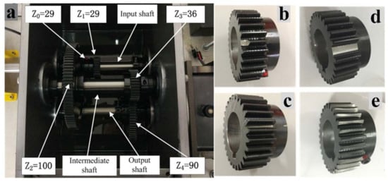
Figure 12.
(a) The parameter of the two-stage parallel gearbox and gears used in the experiment with (b) a chipped tooth, (c) a tooth root crack, (d) a broken tooth, and (e) tooth surface abrasion.
4.2. Tooth Root Crack
The collected original signal of the tooth root crack in the experiment is shown in Figure 13, where impulsive signatures cannot be found in the temporal waveform. It can be only seen in the spectrum that the calculated meshing frequency is about 864 Hz. The reason is that the original signal of the faulty gear is generally influenced by AM/FM components and the additive noise. It is thus difficult to distinguish the condition of the gears based on the above observation.
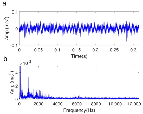
Figure 13.
The original signal of the gear with a tooth root crack: (a) temporal waveform (b) the FFT spectrum.
The decomposed BLIMFs with VMD are shown in Figure 14a. The cyclical impulsive sub-band component (BLIMF2) can be clearly seen. Then, MID is used to further identify the modulation signatures in this BLIMF2. The result of the of BLIMF2 is given in Figure 15a, where the modulation frequency (or cyclic frequency) and its multipliers can be clearly observed. The cyclic frequency is 29.13 Hz and is equal to the rotating frequency of the input shaft, which shows that those impulsive signatures were induced by a local defect in the gear. In addition, the carrier frequency is in nature dominated by the first-order gear meshing frequency (about 850 Hz). Therefore, the failure of the gear on the input shaft has also been demonstrated.
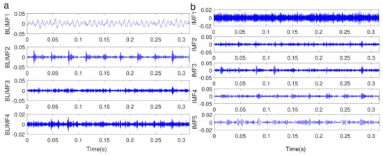
Figure 14.
The decomposed BLIMFs using VMD (a) and IMFs using EMD (b) from the signal of the gear with a tooth root crack.
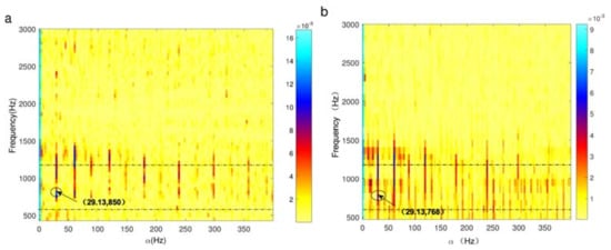
Figure 15.
The of BLIMF2 (a) and IMF3 (b).
The decomposed IMFs with EMD are shown in Figure 14b, where we can find that the cyclical impulsive component (IMF3) is detected. The of IMF3 is given in Figure 15b. It can be seen that the modulation frequency (the cyclic frequency) is also 29.13 Hz, which is equal to the rotating frequency of the input shaft. However, the carrier frequency represents the first-order gear meshing frequency (about 768 Hz). The carrier frequency is not identified in this case. It is obvious that a better result can be achieved using the proposed method than that of EMD combined with MID.
4.3. Chipped Tooth
The original signal of the chipped tooth is illustrated in Figure 16. Although the chipped tooth defect is much severe than the tooth root crack, there are no other meaningful signatures found in the time-domain waveform and its spectrum, except some slight impulsive components in the original signal.
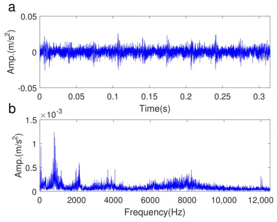
Figure 16.
The original signal of the gear with a chipped tooth (a) temporal waveform (b) the FFT spectrum.
The decomposed BLIMF components with VMD are shown in Figure 17a. Similarly, VMD can not only extract the periodic impulsive component (see BLIMF2), but also well-separate the signal and noise to some extent. The MID of BLIMF2 is given in Figure 18a, where the modulation frequency (cyclic frequency 29.13 Hz) is also equal to the rotating frequency of the input shaft. In addition, the carrier frequency is in nature dominated by the first-order gear meshing frequency (about 850 Hz). Figure 17b shows IMFs achieved using EMD, where we can find that EMD also extracts the periodic impulsive component (see IMF4). It can be easily found in the MID of IMF4 given in Figure 18b that the modulation frequency (cyclic frequency) is also 29.13 Hz and the carrier frequency roughly dominates around 800 Hz. Obviously, the proposed method can achieve a better result than that of EMD combined with MID.
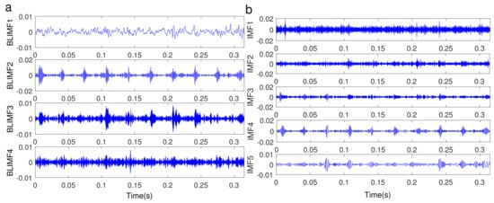
Figure 17.
The decomposed BLIMFs using VMD (a) and IMFs using EMD (b) from the signal of the gear with a chipped tooth.
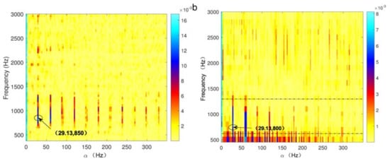
Figure 18.
The of BLIMF2 (a) and IMF4 (b).
In addition, it can be found in the pigmentation directly illustrated in the bi-frequency plot of MID shown in Figure 15a and Figure 18a that the color is darker in Figure 18a due to the severe chipped tooth defect in comparison with the slight tooth root crack. Therefore, to some extent, the severity of gear faults can be judged by observing the pigmentation of the modulation spectrum intensity distribution.
4.4. Tooth Surface Abrasion
The original signal of tooth surface abrasion is displayed in Figure 19. Although it can be found in the frequency domain that the original signal of the gear is mainly combined with the low frequency component near the 1730 Hz resonance band, it is still difficult to judge the running state of the gear.
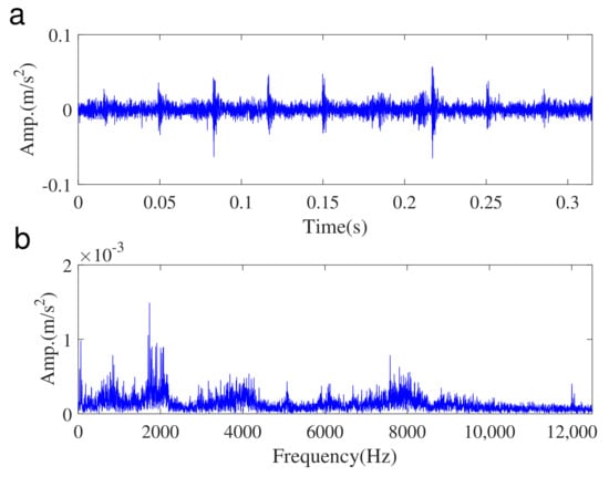
Figure 19.
The original signal of tooth surface abrasion (a) temporal waveform (b) its spectrum.
Once more, the decomposed BLIMF components using VMD are shown in Figure 20a, where periodical impulsive characteristics can be obviously found from the second and the third sub-signals. The IMFs achieved by EMD are illustrated in Figure 20b, where some periodical impulsive information can be also found from the second IMF. The MID of BLIMF2 is shown in Figure 21a, where the modulation frequency (equal to the 29.13 Hz cyclic frequency) and its harmonics can be clearly found. Most importantly, the carrier frequency (about 1750 Hz) is approximate to the double meshing frequency in this case, which is well in accordance with the signatures induced by gear surface abrasion. The MID of IMF2 is shown in Figure 21b. MID combined with EMD cannot identify the modulated frequency and the carrier frequency in this case. This demonstrates that the proposed technique can well-differentiate different gear defects.
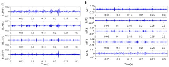
Figure 20.
The decomposed BLIMFs using VMD (a) and IMFs using EMD (b) from the signal of the gear with tooth surface abrasion.
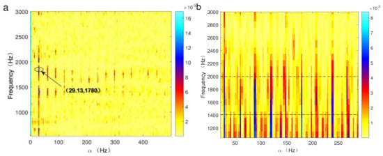
Figure 21.
The of BLIMF2 (a) and IMF2 (b).
4.5. Broken Tooth
In this case, the original signal of a broken tooth is illustrated in Figure 22. In Figure 23a,b, the decomposed BLIMFs and IMFs using VMD and EMD are separately found, where impulsive components can be also seen from BLIMF1 and IMF2. Subsequently, BLIMF1 and IMF2 are analyzed using MID, whose results are given in Figure 24a,b, respectively. It can be found that the modulation frequency and its harmonics are successfully detected once again using the proposed technique, while the carrier frequency is also identified as the meshing frequency (about 850 Hz) in this case. The modulation frequency and its harmonics can be detected using EMD and MID in Figure 24b. The carrier frequency is not identified in this case. It can be found in Figure 24a that the pigmentation of MID is much darker than those in Figure 15a and Figure 18a, since the broken tooth defect is more severe than the chipped tooth and tooth root crack defects.
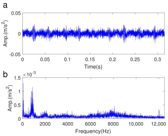
Figure 22.
The original signal of a broken tooth (a) temporal waveform (b) the FFT spectrum.
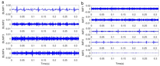
Figure 23.
The decomposed BLIMFs using VMD (a) and IMFs using EMD (b) from the signal of the gear with a broken tooth.
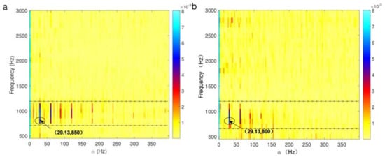
Figure 24.
The of BLIMF1 (a) and IMF3 (b).
5. Conclusions
A hybrid demodulation approach has been proposed for detecting defects in a multistage gearbox using variational mode decomposition and modulation intensity distribution. Variational mode decomposition is used as a pre-processing technique prior to modulation intensity distribution. The reduced frequency aliasing effect of variational mode decomposition is evaluated, which demonstrated that variational mode decomposition is very useful for separating noise and harmonic components. Moreover, the influences of spectral coherence density and spectral correlation density on the modulation intensity distribution have been also investigated. The effectiveness and noise robustness of the proposed method have been well-verified using a simulated signal compared with the empirical mode decomposition algorithm associated with modulation intensity distribution. The merits of the presented technique are as follows: (i) variational mode decomposition can effectively separate noise and harmonic components in the original signal due to its good reduced frequency aliasing effects; (ii) modulation intensity distribution can numerically identify the hidden cyclostationary signatures in the bi-frequency domain and thus can well-differentiate different gear defects; and (iii) the pigmentation visually illustrated in modulation intensity distribution plots can be adopted to quantitatively detect gear defects. The effectiveness of the proposed hybrid demodulation method has been well-verified with simulated and four experimental tests corresponding to different gear health conditions. The results show that the performance of the presented method is also better than that of empirical mode decomposition combined with modulation intensity distribution.
Besides this, a new technique that has been developed to automatically select the optimal components achieved by variational mode decomposition will be reported in future work. Model-based techniques are another important method for fault diagnosis. A comparison between the model-based technique and the proposed signal-based technique will be also considered in the future.
Author Contributions
C.H., J.Y., S.Z. and Y.W. proposed the idea and designed the experiments. C.H. carried out the experiments and analyzed the data. C.H. and S.Z. drafted the paper. C.H. and Y.W. revised the paper.
Acknowledgments
The major part of the study was supported by the project of the National Natural Science Foundation of China (51475098 and 61463010) and the Guangxi Natural Science Foundation (2016GXNSFFA380008). The High Level Innovation Team of Colleges and Universities of Guangxi and the Excellent Scholar Program are gratefully acknowledged. This work is also partially supported by the Recruitment Hundred-Talent Program of Global Experts and the Innovation Project of Guangxi Graduate Education (YCSW2017136).
Conflicts of Interest
The authors declare no conflict of interest.
References
- Zhang, D.; Yu, D. Multi-fault diagnosis of gearbox based on resonance-based signal sparse decomposition and comb filter. Measurement 2017, 103, 361–369. [Google Scholar] [CrossRef]
- Li, Z.; Yan, X.; Yuan, C.; Peng, Z.; Li, L. Virtual prototype and experimental research on gear multi-fault diagnosis using wavelet-autoregressive model and principal component analysis method. Mech. Syst. Signal Process. 2011, 25, 2589–2607. [Google Scholar] [CrossRef]
- Jing, L.; Zhao, M.; Li, P.; Xu, X. A convolutional neural network based feature learning and fault diagnosis method for the condition monitoring of gearbox. Measurement 2017, 111, 1–10. [Google Scholar] [CrossRef]
- Chen, J.; Patton, R.J. Robust Model-Based Fault Diagnosis for Dynamic Systems; Kluwer Academic Publishers: Dordrecht, The Netherlands, 1999. [Google Scholar]
- Ding, S.X. Model-Based Fault Diagnosis Techniques: Design Schemes, Algorithms, and Tools; Springer: Berlin/Heidelberg, Germany, 2008. [Google Scholar]
- Dalpiaz, G.; Rubini, R.; D’Elia, G.; Cocconcelli, M.; Chaari, F.; Zimroz, R.; Bartelmus, W.; Haddar, M. Advances in Condition Monitoring of Machinery in Non–Stationary Operations; Springer: Berlin/Heidelberg, Germany, 2014. [Google Scholar]
- Feng, Z.; Zhang, D.; Zuo, M.J. Planetary gearbox fault diagnosis via joint amplitude and frequency demodulation analysis based on variational mode decomposition. Appl. Sci. 2017, 7, 775. [Google Scholar] [CrossRef]
- Nacib, L.; Saad, S.; Sakhara, S. A comparative study of various methods of gear faults diagnosis. J. Fail. Anal. Prev. 2014, 14, 645–656. [Google Scholar] [CrossRef]
- Fan, X.; Zuo, M.J. Gearbox fault detection using Hilbert and wavelet packet transform. Mech. Syst. Signal Process. 2006, 20, 966–982. [Google Scholar] [CrossRef]
- Huang, N.E.; Shen, Z.; Long, S.R.; Wu, M.C.; Shih, H.H.; Zheng, Q. The empirical mode decomposition and the Hilbert spectrum for nonlinear and non-stationary time series analysis. Proc. R. Soc. Lond. A Math. Phys. Eng. Sci. 1998, 454, 903–995. [Google Scholar] [CrossRef]
- Wang, Y.; He, Z.; Zi, Y. Enhancement of signal denoising and multiple fault signatures detecting in rotating machinery using dual-tree complex wavelet transform. Mech. Syst. Signal Process. 2010, 24, 119–137. [Google Scholar] [CrossRef]
- Dragomiretskiy, K.; Zosso, D. Variational mode decomposition. IEEE Trans. Signal Process. 2014, 62, 531–544. [Google Scholar] [CrossRef]
- Wang, Y.; Markert, R.; Xiang, J.; Zheng, W. Research on variational mode decomposition and its application in detecting rub impact fault of the rotor system. Mech. Syst. Signal Process. 2015, 60, 243–251. [Google Scholar] [CrossRef]
- Wang, Y.; Markert, R. Filter bank property of variational mode decomposition and its applications. Signal Process. 2016, 120, 509–521. [Google Scholar] [CrossRef]
- Mohanty, S.; Gupta, K.K.; Raju, K.S. Hurst based vibro-acoustic feature extraction of bearing using EMD and VMD. Measurement 2018, 117, 200–220. [Google Scholar] [CrossRef]
- Zhang, S.; Wang, Y.; He, S.; Jiang, Z. Bearing fault diagnosis based on variational mode decomposition and total variation denoising. Meas. Sci. Technol. 2016, 27. [Google Scholar] [CrossRef]
- Urbanek, J.; Antoni, J.; Barszcz, T. Detection of signal component modulations using modulation intensity distribution. Mech. Syst. Signal Process. 2012, 28, 399–413. [Google Scholar] [CrossRef]
- Tian, X.; Gu, J.X.; Rehab, I.; Abdalla, G.M.; Gu, F.; Ball, A.D. A robust detector for rolling element bearing condition monitoring based on the modulation signal bispectrum and its performance evaluation against the Kurtogram. Mech. Syst. Signal Process. 2017, 100, 167–187. [Google Scholar] [CrossRef]
- Zhang, R.; Gu, X.; Gu, F.; Wang, T.; Ball, A.D. Gear Wear Process Monitoring Using a Sideband Estimator Based on Modulation Signal Bispectrum. Appl. Sci. 2017, 7, 274. [Google Scholar] [CrossRef]
- Sawalhi, N.; Randall, R.B. Simulating gear and bearing interactions in the presence of faults: Part I. The combined gear bearing dynamic model and the simulation of localised bearing faults. Mech. Syst. Signal Process. 2008, 22, 1924–1951. [Google Scholar] [CrossRef]
- Antoni, J. Cyclostationarity by examples. Mech. Syst. Signal Process. 2009, 23, 987–1036. [Google Scholar] [CrossRef]
- Staszewski, W.J.; Worden, K.; Tomlinson, G.R. Time–frequency analysis in gearbox fault detection using the Wigner–Ville distribution and pattern recognition. Mech. Syst. Signal Process. 1997, 11, 673–692. [Google Scholar] [CrossRef]
- Antoni, J. Cyclic spectral analysis of rolling-element bearing signals: Facts and fictions. J. Sound Vib. 2007, 304, 497–529. [Google Scholar] [CrossRef]
- Randall, R.B.; Antoni, J.; Chobsaard, S. The relationship between spectral correlation and envelope analysis in the diagnostics of bearing faults and other cyclostationary machine signals. Mech. Syst. Signal Process. 2001, 15, 945–962. [Google Scholar] [CrossRef]
- Liu, H.; Song, B.; Qin, H.; Qiu, Z. An adaptive-ADMM algorithm with support and signal value detection for compressed sensing. IEEE Signal Process. Lett. 2013, 20, 315–318. [Google Scholar] [CrossRef]
- Wu, Z.; Huang, N.E.; Chen, X. The multi-dimensional ensemble empirical mode decomposition method. Adv. Adapt. Data Anal. 2009, 1, 339–372. [Google Scholar] [CrossRef]
- Urbanek, J.; Barszcz, T.; Antoni, J. Integrated modulation intensity distribution as a practical tool for condition monitoring. Appl. Acoust. 2014, 77, 184–194. [Google Scholar] [CrossRef]
- Gardner, W. Measurement of spectral correlation. IEEE Trans. Acoust. Speech Signal Process. 1986, 34, 1111–1123. [Google Scholar] [CrossRef]
- Xiang, J.; Zhong, Y.; Gao, H. Rolling element bearing fault detection using PPCA and spectral kurtosis. Measurement 2015, 75, 180–191. [Google Scholar] [CrossRef]
- Urbanek, J.; Barszcz, T.; Sawalhi, N.; Randall, R. Comparison of amplitude-based and phase-based methods for speed tracking in application to wind turbines. Metrol. Meas. Syst. 2011, 18, 295–304. [Google Scholar] [CrossRef]
- Bartelmus, W.; Zimroz, R. A new feature for monitoring the condition of gearboxes in non-stationary operating conditions. Mech. Syst. Signal Process. 2009, 23, 1528–1534. [Google Scholar] [CrossRef]
© 2018 by the authors. Licensee MDPI, Basel, Switzerland. This article is an open access article distributed under the terms and conditions of the Creative Commons Attribution (CC BY) license (http://creativecommons.org/licenses/by/4.0/).