Abstract
Gratings with complex multilayer strips are studied under inclined incident light. Great interest in these gratings is due to applications as input/output tools for waveguides and as subwavelength metafilms. The structured strips introduce anisotropy in the effective parameters, providing additional flexibility in polarization and angular dependences of optical responses. Their characterization is challenging in the intermediate regime between subwavelength and diffractive modes. The transition between modes occurs at the Wood’s anomaly wavelength, which is different at different angle of incidence. The usual characterization with an effective film using permittivity and permeability has limited effectiveness at normal incidence but does not apply at inclined illumination, due to the effect of periodicity. The optical properties are better characterized with effective medium strips instead of an effective medium layer to account for the multilayer strips and the underlying periodic nature of the grating. This approach is convenient for describing such intermediate gratings for two types of applications: both metafilms and the coupling of incident waves to waveguide modes or diffraction orders. The parameters of the effective strips are retrieved by matching the spectral-angular map at different incident angles.
1. Introduction
There are two different applications of gratings in general. First is a diffraction tool with a period larger than the wavelength, and second is as an engineered film with controlled material parameters. The second type of application requires substantially subwavelength gratings, so that in some ranges of wavelengths and angles they can be described by the effective parameters of a uniform film. For those ranges of wavelengths and angles there are no detectable non-zero diffraction orders. One-dimensional gratings consisting of stacked metal-dielectric strips are investigated for their ability to provide magnetic as well as electric resonances [1,2,3,4]. Such resonances are located in the visible spectrum due to the size of the unit cell—less than 0.5 µm. Effective magnetic permeability appears due to circular currents in the stacked structure. It follows from Maxwell’s equations that the transmission and reflection coefficients for the effective film depend on both the product and the ratio of permittivity and permeability, i.e., on the refractive index and the impedance [5,6]. As for any nonlocal effect, the magnetic response increases with the size-to-wavelength ratio. That is why, in the case of metamaterial applications, we are often at the borderline of applicability of the effective parameter approach [7,8]. Often, the grating can be treated as an effective film at normal incidence but it cannot be at inclined incidence. The boundary angle at a specific wavelength is defined by appearance of the first diffraction order, which is the Wood’s anomaly [9,10,11].
Here we characterize such a grating consisting of a stacked vertical substructure by an effective permittivity and permeability of the strips instead of by a continuous effective layer. The approach captures both the effect of the substructure resulting in an artificial permeability, and the diffraction of a grating, by employing a set of effective parameters for the geometrically defined strips. It should be clear that, as is the case with any effective medium approximation, the model works best in the long wavelength limit compared to the strip dimensions. Note, that the effective layer approach can be applicable only in the spectral range of the zero-order diffraction. Any high-order diffraction would result in a wrong retrieval. The experiments presented here show first diffraction order at 450 nm making effective layer approximation not applicable. It is important to note that a grating with the structured strips can be of great interest for the first type of application, especially as an input/output tool for waveguides. Indeed, the structured strips introduce anisotropy in the effective parameters, which makes it possible to realize different polarization and angular dependences, and this behavior is captured by the proposed model.
For similar grating structures, the permeability and permittivity retrieval process has been previously demonstrated for normal-incidence illumination using rigorous coupled wave (RCW) methods [5,6,12] and using complex transmission and reflection coefficients [3,4]. The retrieval for the effective films, however, cannot be verified conclusively for inclined illumination. This is in large part due to the difficulty arising from the effect of diffraction [8,9]. While diffraction occurs at normal incidence, its higher order effects in the range from 400 nm to 1000 nm are typically masked in the effective layer scheme. Under inclined illumination, the Wood’s anomaly is red-shifted into the visible, higher diffraction orders are no longer hidden, and the effective layer method breaks down.
2. Materials and Methods
In this paper, we study a stacked metal-dielectric grating, shown schematically in Figure 1a, at inclined illumination and develop a method to retrieve an effective anisotropic permittivity and permeability of the strips. The grating is fabricated on a transparent substrate and illuminated with white light at various angles of incidence, while light diffracted from the grating is partially coupled to the waveguiding mode and collected as a function of angle from the edge of the substrate, as shown in Figure 1c. The collected light is then delivered to the spectrometer by a fiber bundle. Additionally, normal incidence transmission and reflection measurements are performed in order to provide some information for spectral positions of resonances. The setup described in Figure 1c will produce a wavelength-angle intensity map. This map will be unique for each angle of incidence and each polarization. The simulation efforts will produce the same intensity maps and transmission spectra to match the experimental spectra by adjusting the unknown strip parameters. Thus, using an iterative procedure where the strip parameters are slightly adjusted individually until the best goodness of fit is obtained, we can determine the proper set of parameters. The fitting is done manually, such that the simulated data appears to visually match the experimental data. This matching process is further detailed in the Results and Discussion section. Here we choose modified rigorous coupled wave (RCW) analysis which is utilized as a package within the Modeled Integrated Scattering Tool (MIST [13]). MIST is a front-end graphical user interface to the SCATMECH C++ library of scattering codes, based on rigorous coupled wave theory [14,15,16], modified to account for anisotropic permittivity and permeability (see Appendix A). With this tool, we are able to model diffraction effects of any order. The matching process must be done for each incident angle and each polarization, including that of normal incidence transmission, and the same unique set of permittivity and permeability functions is required for successful matching. The simulation is quite sensitive to the spectral position, amplitude, and line-shape of the strips’ permittivity and permeability functions. The beauty of this approach also lies in the fact that we need not be concerned with the artifacts in the retrieval caused by the grating periodicity.
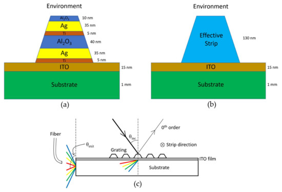
Figure 1.
Sample geometry and experimental setup. Panel (a) shows the vertical substructure of the strip; (b) portrays the replacement of the real structure with an effective strip; (c) depicts the inclined illumination setup, in addition to usual far-field transmission spectroscopy, necessary for retrieving the optical parameters.
Any isotropic medium can be optically characterized by either pair of parameters, index of refraction and impedance , or by permittivity and permeability . All four quantities are causal, complex, and depend on frequency . They are related by
In accounting for a permeability different from unity, it is clear the permittivity and permeability are treated as complex quantities obeying the Kramers–Kronig relations and n and Z are independent functions.
One approach to determine the values for ε and μ of a material, sometimes termed the “effective layer method,” is to use RCW in which the incident light is normal upon the structure. This method however considers the grating as a continuous film and hence, the properties of an effective continuous layer are retrieved. Here, we seek a more complete retrieval which is not restricted to normal incidence, and thus accounts for anisotropy. In this more general situation of incline incidence, a redshift of the Wood’s anomaly into the visible range occurs, which is precisely the wavelength region of our interest and the effective layer retrieval has limited practical use here.
Due to the periodic nature and size of the structure relative to the incident wavelength, an electromagnetic plane wave will undergo diffraction and will transfer some of its power into higher orders. Diffraction effects can be described by the well-known grating equation
where the subscript-free n refers to the transmitted region’s refractive index, is the refractive index in the incident medium, p is the period of the grating, is the wavelength in vacuum, and m is the diffraction order. For the grating under study, our substrate also serves as a waveguide. We wish to simulate the diffraction that occurs due to a periodic grating structure, and the MIST suits our needs for this. MIST includes RCW analysis to simulate the interaction of arbitrarily polarized light with a grating structure of interest. More detail regarding MIST will be given in the subsequent simulation subsection.
The strips of the diffraction grating consist of a total of six layers, essentially forming a metal–insulator–metal (MIM) configuration, which includes adhesion and oxide protection layers. As depicted in Figure 1, each layer of silver lays atop a thin titanium layer, with the metal layers separated by a spacer dielectric, and finally a top protective oxide layer. The die size is 500 μm × 500 μm, with a period of 305 nm and a total height of 130 nm. The bottom and top widths are 155 nm and 80 nm, respectively, which causes an asymmetry to the shape of the two metal strips such that the bottom silver layer is wider than the top silver layer. The metal strips themselves have a thickness of 35 nm, with a 40 nm layer of alumina separating them. Silver is the selected metal due to its low losses at optical frequencies, while alumina has been chosen as the spacer dielectric for its high dielectric constant. It has been shown that the higher dielectric constant spacer is more suitable for magnetic grating metamaterials because it provides better field confinement [17]. Samples have been fabricated on a 15-nm indium-tin-oxide- (ITO) coated fused silica substrate using conventional electron beam lithography (EBL) techniques. The ITO layer is used primarily to provide conduction during EBL. Note that a trapezoidal shape of the cross-section is due to the applied fabrication protocol [6]. After development of the exposed resist, titanium, silver, and alumina layers are deposited by electron beam evaporation. A 3-nm layer of titanium is evaporated before each silver layer to provide good adhesion, making the samples more robust, but lowering the quality of the plasmonic resonances. It is worth mentioning that the roughness and grating quality have been found to be significantly affected by deposition rate [18]. This in turn can affect the optical characteristics of the sample. Specifically, lower deposition rates for gratings and other finer features tend to yield smoother and better-quality nanostructures, as opposed to higher deposition rates giving better quality continuous films. As such, a low deposition rate of 0.1 nm/s has been used. A final liftoff process in acetone is performed revealing the intended grating structure. Figure 2 shows a scanning electron microscopy (SEM) micrograph of the top view of the sample.
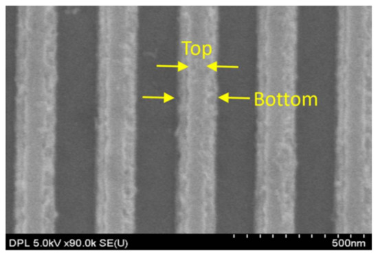
Figure 2.
Scanning electron microscopy (SEM) micrograph of meta-grating sample. Note the trapezoidal shape.
Upon successful fabrication, the sample is used in conjunction with the optical scheme described in Figure 1c. Under normal incidence illumination, diffraction does occur for shorter wavelengths; however, the nonzero orders are trapped in the glass substrate by total internal reflection, and as a result, the detector only detects zero-order diffraction. Supercontinuum white light pulses converted from 800-nm pump (Figure 3) of either transverse electric (TE) or transverse magnetic (TM) polarization illuminate the sample at differing angles of incidence, relative to the sample surface normal. The spectra of the transmission through the substrate at incline incidence are used to normalize the spectral response of the samples. Figure 3 gives an example of such spectra at 30°. The laser source stability is 10% and an example of its output at a particular angle through the substrate as well as its stability with time and with different polarizations is shown in Figure 3. Upon striking the grating, light diffracts at many angles. These diffracted rays are waveguided by total internal reflection through the substrate only in the negative direction. The intensities are collected via a scanned fiber of core diameter 500 μm located a distance of 0.5 mm from the substrate edge, and is subsequently delivered to an imaging spectrometer, whose spectral resolution is 1.5 nm. Note the angular resolution of measurement is 0.5° The output intensity will then be a function of both the angle and wavelength in a spectral-angular intensity distribution (Figure 1c). We ignore rays that propagate in the positive direction which may eventually return to the detector by means of many internal reflections. The reason for this is that, with the angles of incidence used, these rays will not undergo total internal reflection within the substrate, and due to significant loss from many of these repeated reflections, they contribute several orders of magnitude less signal. The process is repeated for incident angles of 30°, 40°, 50°, and 60°, and for two linear polarizations (TE or TM) for a total of eight spectral-angular intensity maps. What follows is a matching process utilizing simulation methods for both normal incidence transmission (zero-order diffraction) as well as the spectral-angular map (nonzero-order diffraction).
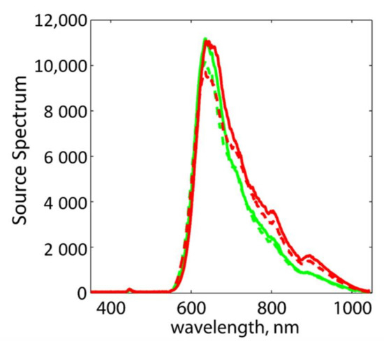
Figure 3.
Substrate transmission at 30° incline, showing the stability of the source output spectra. These spectra are collected for each angle of incidence and used later for normalizing procedures. Green and red lines represent TM and TE polarizations, respectively. The dashed variants show the stability of each after one hour.
Note, that in past retrieval schemes, the grating is approximated as an effective layer and far field transmission and reflection simulations are matched to experimentally observed data (for example [1,2,3]). The type of simulation, that is based on RCW methods, allows retrieval of the complex transmission and reflection coefficients, which can then in turn be used to calculate the permittivity and permeability, albeit as a continuous effective layer. In reality, since a periodic structure is used, diffraction occurs at normal incidence for where is the substrate refractive index. In our case, this approximately translates to first order diffraction occurring at normal incidence for wavelengths less than 450 nm. Thus the effective layer approximation is valid only for the spectral range where the measured transmittance/reflection only contains zero-order information and the higher (nonzero) orders are not allowed.
In this paper, retrieval of the individual strips’ effective optical properties is accomplished by matching simulation spectral-angular data from the designed waveguiding structure, as well as the normal incidence transmission, to the corresponding set of experimental data. For this we use the RCW model included in the MIST. To describe the interacting system, MIST requires the grating geometry, substrate and superstrate media, incident light wavelength, polarization, and angle of incidence, as well as the optical properties of the strips. Despite the strips consisting of several metal and dielectric layers, we model the strip as a single unit—the effective strip. All the roughness and crystal quality of the materials are included in the effective parameters. The physical dimensions of the strip are those of the real sample, while the effective parameters of the strips are what we seek, and are also the only set of unknown variables. A unique ability of MIST is that it allows the calculation of any arbitrary diffraction order as well as anisotropic magnetic behavior. In this way, we can provide any tabulated dispersion for a range of frequencies for all permittivity and permeability functions. We briefly mention that, for inclined illumination and the wavelengths we use, it is only necessary to analyze a single diffraction order. Namely , the first order, contributes to a meaningful relative intensity at the output. Minus is due to geometrical convention. The other orders either do not exist, or their efficiencies are negligible—as is the case for orders higher than the first order.
Any arbitrary complex function for both ε(λ) and μ(λ) can be supplied to MIST. Typically, in anisotropic media the electric (magnetic) susceptibility and therefore permittivity (permeability) functions exist in the form of a second rank tensor. Each function will uniquely have three nonzero effective medium components, namely:
where each component is a complex and frequency dependent quantity. The off-diagonal components are zero due to the geometry of the grating. Figure 4 shows the coordinate system being used.
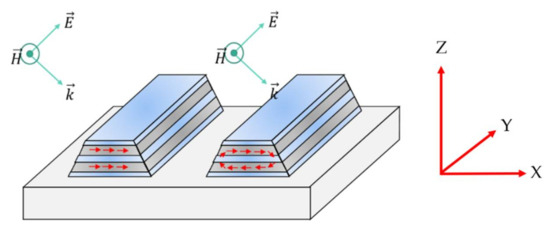
Figure 4.
Representation of the actual trapezoidal shape of the grating due to fabrication limitations. A TM-polarized beam is incident at an incline; depending on frequency, either a symmetric (Left) or antisymmetric (Right) mode may be excited. Note that the strips are still considered to be infinite in the y-direction.
If only normal incidence transmission is utilized, it is not guaranteed that all the components of the effective permittivity and permeability of the strips are involved. We find that there are several functions that will provide a suitable match to the transmission data. Additionally, the z-components of the permittivity and permeability are concealed at normal incidence, and we only begin to noticeably detect their effect at larger angles of incidence. Only when the normal incidence matching is used in conjunction with the incline illumination results can we obtain the correct set of effective optical properties of the system.
We next discuss the physical grounds for the accepted fitting formulas on the six unknown components. Different polarizations and incident angles are used to isolate and better capture specific components of the effective permittivity and permeability. Moreover, we find there is a significant polarization dependency on the output, due to the strong resonance occurring with the TM polarization and lack of resonance with TE polarization. Figure 4 illustrates that when the E-field lies along the strip axis, this TE-polarized wave is unable to produce any resonant effects, and thus the strip will behave as a diluted metal. In this case the observable permeability is unity, hence, . We note that by keeping the x- and z-components of the effective permeability, nonmagnetic response is an enforced condition. Meanwhile the observable component when using TE polarization will be strictly that of εy, though as we shall see it differs moderately from the standard EMT of a dilute metal. Hence by using TE polarized light, we can isolate the y-component of the permittivity.
On the other hand, when the incident wave is TM polarized, both symmetric and antisymmetric resonant current modes may be excited. Here we see no effect from either μx or μz due to the fixed direction of the magnetic field along the strip. However, a magnetic dipole response manifests with μy via the oscillations of the light wave’s magnetic field. In fact, it is this magnetic resonance which is precisely the desired effect that we hope to observe. The electric permittivity takes form with εx and εz. It should be clear that with normal incidence measurements, the total anisotropy cannot be recovered. Let us now summarize the results provided by polarization:
where the left matrices are sensed with TE polarization and the right matrices are sensed with TM polarization.
It is only and which display resonant behavior, while shows dilute metal characteristics, and and are simply unity. The z-component of the permittivity is not expected to be resonant in the visible spectrum, though its form via simulation will turn out to be that of a somewhat modified Drude function.
There are, then, a total of four unknown parameters that must be modeled. For the TM resonant modes, both the permittivity and permeability functions have asymmetry of the resonance (see, for example [5,18]). Because of this asymmetry, we choose a transversal optical longitudinal optical (TOLO) oscillator function [19] to describe these modes, rather than a classical Lorentzian. These take the form
and
where, after matching, we find = 0.11, , , , and , while for μy, = 0.13, , , , and . Here, is the photon energy. For these dielectric functions to remain physical with and , the constraint must be satisfied.
Meanwhile, to model “diluted metal” for both and , we use a Drude function of the form
where and for we have , , and , while for we have , , and . It is interesting to note that without the large offset parameter, , for the Wood’s anomaly peak will be hidden in transmission spectra.
The details regarding the exact spectral position, amplitude, and sharpness of each resonance and the parameters for the dielectric functions are initially unknown. Therefore, an iterative technique must be performed until an acceptable match has been made for both normal incidence transmission as well as for each angle of incidence and polarization of the spectral angular map. As previously mentioned, TE polarization is employed to uniquely determine . As an example, for this case there are three parameters from the Drude relationship above that must be found. Values for each parameter are initially chosen with some physical justification, and subsequently the simulation is completed for all angles of incidence. The relative intensities of the spots on the spectral-angular map are analyzed, and one at a time the parameters are changed gradually to provide a closer match in intensity. The same parameters must also satisfy the normal incidence transmission for this polarization. In this way, we find the values that describe the y-component of the permittivity.
On the contrary, the TM polarization case is considerably more complex due to the fact that not one, but three components of permittivity and permeability affect the outcome, namely , , and . Additionally, the resonant functions each contain five fitting parameters resulting in several more degrees of freedom. However, there exist two resonances in the transmission spectra (Figure 5). The shorter wavelength resonance is associated with electric permittivity function and the longer wavelength resonance with magnetic permeability function. The following section provides details of the results of this matching procedure.
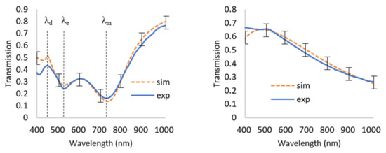
Figure 5.
Normal incidence transmission for TM (Left) and TE (Right) polarizations. Note that only is responsible for TE spectra, while TM spectra depends on , , and . With TM polarization, , , and correspond to the Wood’s anomaly (diffraction threshold), electric resonance, and magnetic resonance, respectively. Data is matched by providing incremental adjustments to the parameters of each dielectric function. Note that the set of parameters providing agreement here must also provide satisfactory matching for the spectral-angular data. Error bars in simulated spectra reflect ±5% uncertainty.
3. Results and Discussion
The designed grating is considered optically magnetic due to the ability of TM-polarized visible light to excite asymmetric circulating currents in the metal layers, thereby giving rise to a magnetic moment directly along the strips of the structure. This is fundamentally a result of the oscillating magnetic field along the strip axis and Faraday’s law. Both a symmetric current mode and an asymmetric mode may be excited, representing an electric and magnetic resonance, respectively. The spectral position of the magnetic resonance has been previously demonstrated to be a result of the effective width of the grating (or fill factor) [20], though the normal incidence transmission local minima provide a baseline of sorts to determine the spectral locations for both and As seen in Figure 5 the TM polarized transmission displays two local minima; the first, and the second, . These represent the electric and magnetic resonances, respectively, and specifically refer to and . Therefore, we have in mind a starting point for the spectral location of the resonances of the permittivities and permeability. The sharp peak at is due to the Wood anomaly and is not observed in simulation until is properly determined. As an example, if is given a constant nonabsorbing value of , the sharp peak at is washed out; in this case a static offset to the real part of approximately is required for the diffraction threshold peak to appear.
The simulation results for the spectral-angular map are performed with the experimental values of the period of the grating, the location of the incident beam relative to the waveguide edge, as well as the substrate thickness and refractive index (see Figure 6). In Figure 6 we also explain why the spectral angular maps to be seen in Figure 7 and Figure 8 are not continuous. Indeed, depending on the incident beam positions relative to the substrate edge, there are three possible scenarios. The beam at a particular wavelength may either hit the corner and split between upward and downward as shown in Figure 6a, or propagate in one of two directions, upward or downward. If the beam goes upward it makes a gap in the down side as indicated by arrows on Figure 6b. We emphasize that these aforementioned parameters taken from experiments control only the location and the size of the “spots” seen in the spectral-angular maps in Figure 7 and Figure 8. More importantly, the permittivities and permeabilities are mainly responsible for the intensities of these spots.
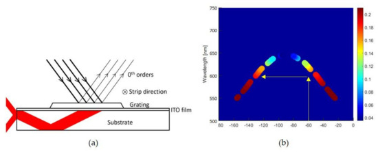
Figure 6.
The geometry of the sample affects the output; this is shown for parallel rays interacting with the grating (a). Note, that depending on the incident beam positions relative to the substrate edge there are three possible scenarios, these rays may either hit the corner and split between upward and downward as shown in (a), or propagate in one of two directions, upward or downward. If the beam goes upward it makes a gap in the down side (b). Map (b) is an angular extension of Figure 8b SIM TM 40°, as an example; the gap at −60° is pointed by arrow.
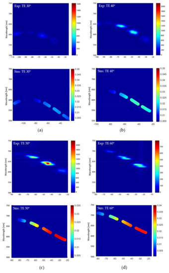
Figure 7.
Experimental (top panels) and simulated (bottom panels) spectral-angular map of TE polarized incident light for incident angles 30° (a), 40° (b), 50° (c), and 60° (d). The intensity scales are in the same units for all maps of the TE polarization. Simulated data are matched to experimental data by considering maximum intensity in a spot.
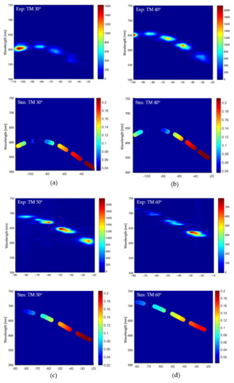
Figure 8.
Experimental (top panels) and simulated (bottom panels) spectral-angular map of TM polarized incident light for incident angles 30° (a), 40° (b), 50° (c), and 60° (d). The intensity scales are in the same units for all maps of the TM polarization. Simulated data are matched to experimental data by considering maximum intensity in a spot.
To retrieve the effective optical properties, we begin with an initial guess for each parameter in the TOLO and Drude wavelength-dependent functions. This guess is influenced by the experimental transmission data and gives a starting point for the resonant spectral positions as well as the non-resonant spectra modeled as a diluted metal. These functions provide a value for permittivity and permeability at each wavelength, and are then fed to the MIST GUI which operates on each value using the modified RCW code. By varying the conditions, it will output either a transmission spectrum at normal incidence or a spectral-angular map—both must be performed. One by one, each parameter of the TOLO and Drude functions are iteratively adjusted until both the transmission and spectral-angular maps at all angles both match satisfactorily based on eye evaluation. This process is guided by the most sensitive parameters for the resonant spectral position, amplitude terms, followed by the spectral width term, and lastly the asymmetrical parameters. For example, to obtain , and , we use the TM experimental data. Realizing that is responsible for the magnetic resonance and mainly responsible for the electric resonance, both amplitude and spectral position terms are initially chosen such that they best match the transmission data for the respective minima. The spectral positions for the resonant functions are initially chosen to be the same as those of the transmission minima. Note, these positions may not exactly coincide after finalizing the matching. Since the two resonances are not spectrally separated by a significant amount, increasing the amplitude of, for example, can have an impact on the simulated transmission’s local electric minima, and vice versa.
Matching is assessed for the spectral-angular maps by comparing each spot’s relative intensity. Upon doing so, we have best matched the simulated spectra to the experimental data. Thus, we have found each component previously discussed, namely, , and . Meanwhile and are set equal to unity as an enforced condition. Again, note that physical arguments are used to evaluate suitable functions, such as exhibiting a behavior similar to that of a dilute metal—a result of the non-resonant TE mode. The result of the normal incidence matching is shown in Figure 5, while all spectral-angular matching results for varied angles and polarizations are shown in Figure 7a–d and Figure 8a–d. The results in Figure 7 and Figure 8 all account for uncertainty in the spectral-angular position by allowing each data point to have a specific radius, such that it reflects the experimental data uncertainty. Furthermore, based on Figure 9 and Figure 10, Figure 11 shows the functions chosen to satisfy matching of the experimental data. It is emphasized that the matching in Figure 5 and Figure 7 and Figure 8 are not independent of one another, but rather the same set of permittivity and permeability must provide agreement for both.
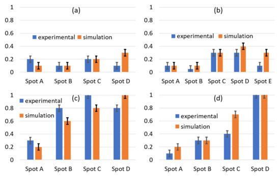
Figure 9.
Spectral-angular data conversion for TE of each prominent “spot” to 1D column graph. The labels A, B, C, D, and E refer to the spots from left to right in Figure 7 in each intensity map at different incident angles: 30° (a), 40° (b), 50° (c), and 60° (d). Error bars reflect a 10% uncertainty. All intensities are on a relative zero to one scaling system.
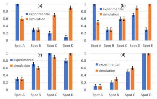
Figure 10.
Spectral-angular data conversion for TM of each prominent “spot” to 1D column graph. The labels A, B, C, D, and E refer to the spots from left to right in Figure 8 in each intensity map, while panels a-d correspond to different incident angles 30° (a), 40° (b), 50° (c), and 60° (d). Error bars reflect a 10% uncertainty. All intensities are on a relative zero to one scaling system.
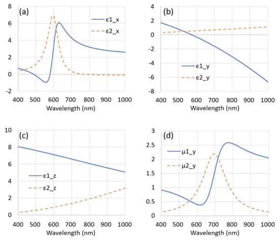
Figure 11.
Retrieved parameters of the permittivity and permeability via our methods; note μx and μz (not pictured) are unity. (a–c) respectively show the x-, y-, and z-components of the permittivity while (d) shows the y-component of the permeability. ε1 and μ1 refer to real parts, while ε2 and μ2 refer to imaginary parts of the corresponding function.
To obtain a successful match, both normal incidence transmission and waveguided inclined illumination simulation data should agree with the experimental results. It is extremely challenging to simultaneously have both agree with a high degree of accuracy, especially using singly resonant Lorentzian-type functions with a limited number of fitting parameters. An improved match with the spectral-angular map will tend to significantly deteriorate the normal incidence match, and vice versa. Here we have attempted to minimize the degrees of freedom for more convenient fitting and to demonstrate the retrieval process.
The matching of the normal incidence data alone is straightforward. For TM polarization, one typically associates the permeability strictly with the longer wavelength (magnetic) resonance λm and the x- and z-permittivities with the shorter wavelength (electric) resonance. Incremental adjustments are made to the respective amplitudes, spectral positions, and sharpness of each function. The same process is done for TE polarization for the y-component of the permittivity. However, the difficulty that arises is that these functions must now also provide agreement with the spectral-angular data. Since only one component is responsible in the TE polarization, agreement with the spectral-angular map here occurs rather naturally. On the other hand, due to the TM polarization containing three functions that are responsible for the output, the agreement is not as straightforward. At this stage, further adjustments to these three functions are made such that the spectral-angular maps agree.
At first glance, the matching for the spectral-angular map is difficult to discern visually. To further clarify the matching success, in each map, we label each spot and characterize it by how much average relative intensity it receives. In this way, the three-dimensional plot can be reduced to a one-dimensional column graph, as shown in Figure 9 and Figure 10. This is reasonable because only the material properties can provide the correct relative intensities, while geometry and diffraction dictate the angle and wavelength possible at each location. Since the material properties (i.e., permittivity and permeability) are responsible for the intensity of each spot, while the geometry and diffraction provide the spectral-angular location, this reduced one dimensional plot is best representative of the fitting, as this extracts only the desired effective optical parameters from the rest of the information producing Figure 7 and Figure 8.
We can then compare intensities of each spot. Note that one set of permittivity and permeability must satisfy all sets of data, including normal incidence data as shown in Figure 5, which makes matching trustable.
As one can see from the comparative presentation in Figure 9 and Figure 10, the agreement between the experiment and simulations are not ideal for some spots. For example, spots 3 and 4 in the TM 30° incident angle trial, which correspond to exit angles of approximately −65° and −45°, respectively, we note there is simulated radiation that is not quite detected experimentally. On the contrary, most all other spots at other incident angles are in close relative agreement. With slight deviations of the current optical properties’ spectral position, amplitude, sharpness or symmetry, the “overall matching” drastically reduces. Here, overall matching simply translates to the matching of all eight spectral angular maps and the normal incidence transmission. For example, a 5-nm deviation in spectral position of the permeability may improve the matching for spots 3 and 4 in the TM 30° incident angle match, but subsequently worsen several other spots for other angles. Hence with the presented optical parameters (Figure 11), the best “overall match” was obtained.
Obtaining a good fit for all angles of incidence, in addition to normal incidence transmission gives all components of the permittivity and permeability of the effective strips. As always, the fitting is limited by the accuracy, to which we know the exact geometry, roughness, and any fluctuations that occur throughout the real grating structure.
The previous effective layer method works if normal incidence applications are required in which only the wavelengths longer than Wood anomaly are considered. This turns out normally to be reasonable for the visible spectrum. However, if one is trying to avoid the issue of diffraction in the wavelength range of interest, the period of the grating should be pushed to smaller dimensions, shifting the first diffraction event to shorter wavelengths. This begins to present a significant fabrication challenge. Even with a decreased period dimension, when oblique incidence is used with the metamaterial, the Wood anomaly is red shifted into the visible, creating an obvious problem for the effective layer method. In contrast, by using the effective strip retrieval, diffraction is accounted for, the period does not need to be pushed to smaller dimensions, and oblique incidence applications can be realized with the proper set of parameters. We introduce Table 1 below to summarize the comparison.

Table 1.
Comparison between effective layer and strip methods for parameter retrieval.
Note, that the main point of introducing magnetic response is that the two parameters, refractive index and impedance, become independent. If we can describe everything with just electric permittivity, thus n = 1/Z, and magnetic response is absent, meaning μ = 1.
The capability of such a stacked grating material to waveguide the diffracted modes resulting from inclined illumination of the periodic grating surface makes it possible to apply such structures in biosensing. Using this design, the spectrum of the diffracted modes is sensitive to the refractive index of the material on the grating surface. For this reason, any changes in the refractive index due to a biochemical reaction on the surface [21] can be detected with this method. Additionally, upon retrieving the effective strip parameters, one may utilize such a grating design that exhibits a specialized set of optical properties in more practical situations where oblique incidence illumination is natural, such as the improvement of the efficiency in solar cells with unpolarized incident light [22]. Finally, we may generalize the method of parameter retrieval to other periodic nanostructures by using a similar experimental setup and simulation process. With a better understanding of how the effective optical properties of the strips depend on the geometry and materials chosen, it is hoped that further research will allow one to engineer a material with a specific set of optical parameters in mind which do not naturally occur.
4. Conclusions
We demonstrate a new approach for retrieving the effective optical properties of the structured strips of a metamaterial grating. The simulations are performed for an effective grating, implying uniform anisotropic material, using the well-known RCW technique, which is modified to allow magnetic behavior and anisotropy. Notably this expands the relevance of the model to capturing properties for inclined illumination by capturing the anisotropy of the properties of the strips in contrast to the validity at normal incidence only of the effective layer model. Coupling experimental measurements of samples with inclined illumination in addition to normal incidence to a scattering software tool (MIST) allows us to model both inclined and normal incidence illumination and capture relevant diffracted orders. Providing the proper set of complex permittivity and permeability functions, a successful fit to the experimental data will occur. This retrieval method allows for capturing behavior in nonzero diffraction orders. Indeed, the diffraction features observed in the experiment and simulations in Figure 5 at 450 nm have been excluded from the retrieval results in Figure 11 due to the applied approach. Thus our method provides a more broadly relevant effective property extraction for use in applications of magnetic gratings. The coupling of experimental methods to the MIST package is additionally useful in that, once the optical parameters are obtained, one may probe the system via the same simulation environment in other ways to realize applications, such as waveguide-based biosensing, and to optimize grating performance by examining configuration changes. We believe a similar scheme can be useful for two-dimensional gratings [23], i.e., the so-called “fishnet” nanostructure, to obtain their effective unit parameters.
Acknowledgments
Vladimir P. Drachev acknowledges support of this work by Russian Ministry of Education and Science grant RFMEFI58117X0026.
Author Contributions
Vladimir P. Drachev, Augustine M. Urbas and Dean P. Brown conceived and designed the experiments; David P. Lyvers, Kevin M. Roccapriore, Ekaterina Poutrina and Dean P. Brown performed experiments; Thomas A. Germer extended the RCW theory to include magnetic susceptibility, as described in Appendix A, Kevin M. Roccapriore and Thomas A. Germer performed numerical simulations. All authors contributed to overall data analysis and scientific discussions. Kevin M. Roccapriore, Vladimir P. Drachev, David P. Lyvers, Augustine M. Urbas and Thomas A. Germer wrote the manuscript with contributions from all authors. Vladimir P. Drachev supervises the project.
Conflicts of Interest
The authors declare no conflicts of interest.
Appendix A
The RCW code used in this study implements the theory of Moharam et al. [15] as extended by Li [16] to properly account for the Fourier decomposition of the fields in the presence of discontinuities. To account for diagonal anisotropy and magnetic response of the media, the theory was further extended. For transverse electric (TE) polarization, the matrix in Equation (14) of Moharam’s paper [15] in the presence of diagonal ε and is replaced by
where , and , , and are Toeplitz matrices formed from the Fourier coefficients of , , and , respectively. is then replaced by . Similarly, for transverse magnetic (TM) polarization, the matrix in Equation (34) of Moharam’s paper [15] in the presence of diagonal ε and is replaced by
where , and , , and are Toeplitz matrices formed from the Fourier coefficients of , , and , respectively. is then replaced by .
References
- Kildishev, A.V.; Cai, W.; Chettiar, U.K.; Yuan, H.-K.; Sarychev, A.K.; Drachev, V.P.; Shalaev, V.M. Negative refractive index in optics of metal-dielectric composites. JOSA B 2006, 23, 423–433. [Google Scholar] [CrossRef]
- Brown, D.P.; Walker, M.A.; Urbas, A.M.; Kildishev, A.V.; Xiao, S.; Drachev, V.P. Direct measurement of group delay dispersion in metamagnetics for ultrafast pulse shaping. Opt. Express 2012, 20, 23082–23087. [Google Scholar] [CrossRef] [PubMed]
- Drachev, V.P.; Podolskiy, V.A.; Kildishev, A.V. Hyperbolic metamaterials: New physics behind a classical problem. Opt. Express 2013, 21, 15048–15064. [Google Scholar] [CrossRef] [PubMed]
- Ekinci, Y.; Christ, A.; Agio, M.; Martin, O.J.F.; Solak, H.H.; Löffler, J.F. Electric and magnetic resonances in arrays of coupled gold nanoparticle in-tandem pairs. Opt. Express 2008, 16, 13287–13295. [Google Scholar] [CrossRef] [PubMed]
- Smith, D.R.; Schultz, S.; Markoš, P.; Soukoulis, C.M. Determination of effective permittivity and permeability of metamaterials from reflection and transmission coefficients. Phys. Rev. B 2002, 65, 195104. [Google Scholar] [CrossRef]
- Smith, D.R.; Vier, D.C.; Koschny, T.; Soukoulis, C.M. Electromagnetic parameter retrieval from inhomogeneous metamaterials. Phys. Rev. E 2005, 71. [Google Scholar] [CrossRef] [PubMed]
- Yuan, H.-K.; Chettiar, U.K.; Cai, W.; Kildishev, A.V.; Boltasseva, A.; Drachev, V.P.; Shalaev, V.M. A negative permeability material at red light. Opt. Express 2007, 15, 1076–1083. [Google Scholar] [CrossRef] [PubMed]
- Kildishev, A.; Chettiar, U. Cascading optical negative index materials. Appl. Comput. Electromagn. Soc. J. 2007, 22, 172–183. [Google Scholar]
- Nilsson, P.-O. Determination of Optical Constants from Intensity Measurements at Normal Incidence. Appl. Opt. 1968, 7, 435–442. [Google Scholar] [CrossRef] [PubMed]
- Wood, R.W. Anomalous Diffraction Gratings. Phys. Rev. 1935, 48, 928–936. [Google Scholar] [CrossRef]
- Hessel, A.; Oliner, A.A. A New Theory of Wood’s Anomalies on Optical Gratings. Appl. Opt. 1965, 4, 1275–1297. [Google Scholar] [CrossRef]
- Ni, X. PhotonicsSHA-2D: Modeling of Single-Period Multilayer Optical Gratings and Metamaterials. Available online: https://nanohub.org/resources/sha2d (accessed on 11 May 2017).
- Germer, T.A. Modeled Integrated Scatter Tool (MIST). Available online: https://www.nist.gov/services-resources/software/modeled-integrated-scatter-tool-mist (accessed on 17 January 2018).
- Moharam, M.G.; Gaylord, T.K. Rigorous coupled-wave analysis of grating diffraction—E-mode polarization and losses. J. Opt. Soc. Am. 1983, 73, 451–455. [Google Scholar] [CrossRef]
- Moharam, M.G.; Grann, E.B.; Pommet, D.A.; Gaylord, T.K. Formulation for stable and efficient implementation of the rigorous coupled-wave analysis of binary gratings. JOSA A 1995, 12, 1068–1076. [Google Scholar] [CrossRef]
- Li, L. Use of Fourier series in the analysis of discontinuous periodic structures. JOSA A 1996, 13, 1870–1876. [Google Scholar] [CrossRef]
- Cai, W.; Shalaev, V. Optical Metamaterials; Springer: New York, NY, USA, 2010; ISBN 978-1-4419-1150-6. [Google Scholar]
- Drachev, V.P.; Chettiar, U.K.; Kildishev, A.V.; Yuan, H.-K.; Cai, W.; Shalaev, V.M. The Ag dielectric function in plasmonic metamaterials. Opt. Express 2008, 16, 1186–1195. [Google Scholar] [CrossRef] [PubMed]
- Schubert, M.; Tiwald, T.E.; Herzinger, C.M. Infrared dielectric anisotropy and phonon modes of sapphire. Phys. Rev. B 2000, 61, 8187–8201. [Google Scholar] [CrossRef]
- Cai, W.; Chettiar, U.K.; Yuan, H.-K.; de Silva, V.C.; Kildishev, A.V.; Drachev, V.P.; Shalaev, V.M. Metamagnetics with rainbow colors. Opt. Express 2007, 15, 3333–3341. [Google Scholar] [CrossRef] [PubMed]
- Liang, W.; Huang, Y.; Xu, Y.; Lee, R.K.; Yariv, A. Highly sensitive fiber Bragg grating refractive index sensors. Appl. Phys. Lett. 2005, 86, 151122. [Google Scholar] [CrossRef]
- Kruk, S.S.; Wong, Z.J.; Pshenay-Severin, E.; O’Brien, K.; Neshev, D.N.; Kivshar, Y.S.; Zhang, X. Magnetic hyperbolic optical metamaterials. Nat. Commun. 2016, 7, 11329. [Google Scholar] [CrossRef] [PubMed]
- Xiao, S.; Chettiar, U.K.; Kildishev, A.V.; Drachev, V.P.; Shalaev, V.M. Yellow-light negative-index metamaterials. Opt. Lett. 2009, 34, 3478–3480. [Google Scholar] [CrossRef] [PubMed]
© 2018 by the authors. Licensee MDPI, Basel, Switzerland. This article is an open access article distributed under the terms and conditions of the Creative Commons Attribution (CC BY) license (http://creativecommons.org/licenses/by/4.0/).