Robust Optimization for Household Load Scheduling with Uncertain Parameters

Abstract

Home energy management systems (HEMS) face many challenges of uncertainty, which have a great impact on the scheduling of home appliances. To handle the uncertain parameters in the household load scheduling problem, this paper uses a robust optimization method to rebuild the household load scheduling model for home energy management. The model proposed in this paper can provide the complete robust schedules for customers while considering the disturbance of uncertain parameters. The complete robust schedules can not only guarantee the customers’ comfort constraints but also cooperatively schedule the electric devices for cost minimization and load shifting. Moreover, it is available for customers to obtain multiple schedules through setting different robust levels while considering the trade-off between the comfort and economy.

1. Introduction

Residential customers are faced with diverse pricing schemes implemented by utilities to stimulate demand response [1,2,3], and are hence faced with the subsequent problem on how to operate the household appliances to minimize the electricity payment under the premise of human comfort. The growing integration of household generation, mainly intermittent renewable generation, makes this problem even more complex. By integrating advanced automatic control and information and communication technologies, home energy management systems (HEMS) make it possible for residential customers to optimally manage their household appliances, i.e., to shift and curtail household loads to properly respond to the various pricing schemes [4]. Under this background, HEMS have been attracting increasing attention in recent years.

There are many studies that model the household load scheduling problem as a deterministic optimization problem [5,6]. In [7], a detailed home energy management system structure is developed to determine the optimal day-ahead appliances scheduling under hourly pricing and peak power-limiting. In [8], in order to distinguish the energy consumption modes and corresponding status of different appliances, home appliances are assigned dynamic priorities, and a real-time household load priority scheduling algorithm, based on the allocated priority and renewable source availability prediction, is proposed to minimize the cost of energy consumption with customers’ comfort constraints. Aiming at minimizing the electricity bill and customers’ dissatisfaction at the same time, Soares et al. [9] propose a multi-objective genetic algorithm to optimize the time allocation of domestic loads, and similar to the Non-dominated Sorting Genetic Algorithm II, some changes have been introduced in the proposed algorithm to adapt the physical characteristics of the load scheduling problem and improve the usability of results.

However, in these studies, many parameters, such as the time-varying prices, ambient temperature, customer behaviors, etc., are assumed to be obtained through day/hour/minute-ahead forecasting, which contains inevitable uncertainties that will undermine the feasibility and optimality of the load schedules obtained. In order to tackle this issue, many researchers have conducted a large number of works and made very large achievements. In general, these works are divided into the following two methods. One method is to enhance the accuracy of forecast parameters by improving the forecasting methods. In [10], a new hybrid model that combines two well-known methods for short-term power forecasting of a grid-connected photovoltaic plant is introduced. And hourly forecasts of photovoltaic power output show a quite good accuracy and efficiency of the developed hybrid model. In [11], Weron collects a variety of methods and ideas about electricity price forecasting. Although these methods have different strengths and weaknesses, it is proved that these methods have obtained varying degrees of success and forecasting precision. Another method is to make ultimate schedules to withstand the uncertainty through various kinds of uncertain optimizations. In [12], a stochastic scheduling technique is used to handle the uncertainties contained in the energy consumption and runtime of household appliances. In [13], typical uncertain parameters in the day-ahead temperature scheduling for air-conditioning are modeled by membership functions with fuzzy set theory. In [14], normally distributed random variables are used to describe the uncertain parameters, and a chance constrained optimization model is then formulated to accommodate the uncertainties.

Although the aforementioned papers make great success to deal with these uncertain parameters in HEMS, there exists some limitations and shortcomings. Due to the complexity of impacting sources in the forecast model and randomness of human behaviors, some forecast parameters, especially like the ambient parameters and customer behavioral parameters, are still not accurate enough to represent the real environment. Meanwhile, most forecast methods need a large amount of historical data which is difficult or expensive for household customers to obtain. Especially, the stochastic programming accounts for a large part of the uncertain optimization methods. Since the characteristics of heuristic algorithms are widely used in the stochastic programming, it is inevitable that the results will be trapped in local optima and make the iteration rather time-consuming.

Differing form the above studies, this paper applies a robust optimization method to tackle the uncertainties in household load scheduling. In 1973, Soyster firstly gained the solutions under the worst situation of uncertain parameters through linear robust optimization [15]. To decrease the conservatism of linear robust optimization, Ben-Tal et al. [16] proposed the adjustable robust optimization counterpart. Bertsimas and Sim [17,18] extended the robust optimization by introducing an adjustable factor to reflect the different choices from the uncertain parameters set. The robust optimization proposed by Bertsimas has some advantages in handling the uncertainties in parameters: through modeling the uncertain parameters varying in a given uncertainty set, it avoids complex random variables which are subjected to the probability distribution or fuzzy membership function, and it maintains the linearity of the problem so that the global optimal solution can be obtained by a linear programming solver. Additionally, based on setting different values of the factor, it can flexibly control the conservative levels of the results. Based on these, quite a few works [19,20,21] pay significant attention to robust optimization in HEMS. Thus, this robust method is applied in HEMS to solve the scheduling problem with uncertainties.

In this paper, a home energy management system equipped with photovoltaic generation and an energy storage device is established. A household load scheduling with uncertain parameters is formulated to minimize the electricity bill of customers and operates under the comfort constraints. Specifically, the main contributions of this paper can be summarized as follows:

• Two typical examples of uncertain parameters, outdoor temperature and hot water demand, are modelled as uncertainty sets, based on which household load scheduling problem with uncertainties is formulated. For researching the uncertainties, the uncertain parameters are presented in the form of interval numbers.
• A robust optimization method is applied to deal with the uncertainties in the comfort constraints. The robust counterpart transformation is the key component of robust optimization. Via deducing the robust counterpart, the original scheduling problem is transformed into a mixed integer linear programming problem, of which the global optimum can be found by mature tools, such as CPLEX. The proposed method avoids the time-consuming iterations in many other uncertain optimization methods.
• An uncertainty analysis that quantifies the violation degree of the comfort constraints is designed and conducted to test the proposed method. The results show that the complete robust schedules is able to guarantee that the comfort constraints will not be violated. Moreover, schedules with different robust levels can be obtained to make a trade-off between the comfort violation and electricity payment.

This paper is organized as follows: Section 2 introduces the mathematical model of the home energy management system, including the uncertain parameters, objective function, and constraints; Section 3 introduces the robust optimization method and completes the derivation of the robust counterpart; and, finally, the simulation results are presented and analyzed in Section 4 and Section 5.

2. Mathematical Model

2.1. Uncertain Parameters

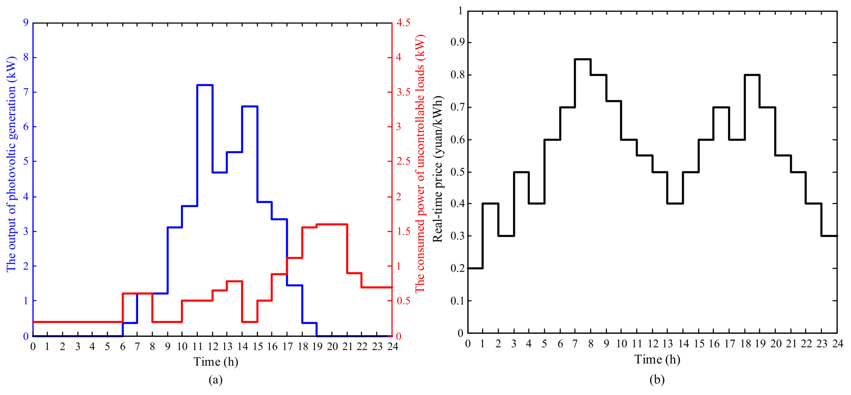
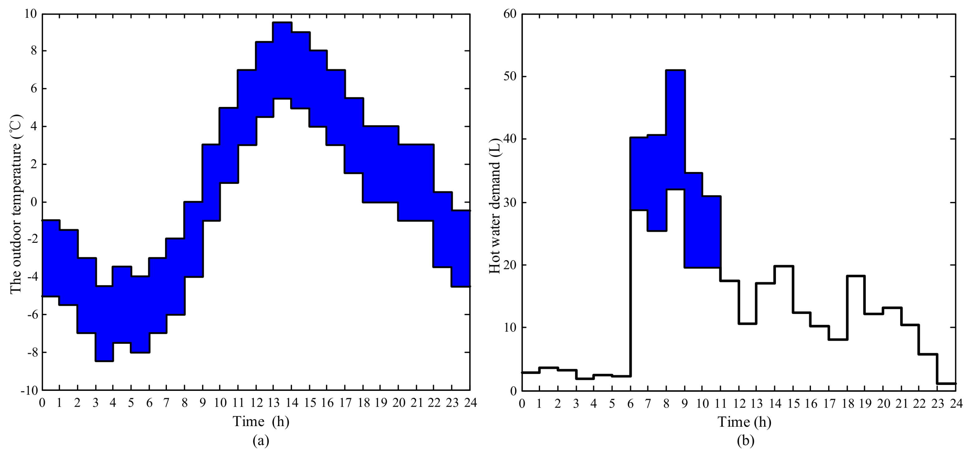
In household load scheduling, the outdoor temperature and hot water demand for the next day are representative uncertain parameters that are closely affected by the randomness in the environment and human behaviors and cannot be predicted precisely in practice. Thus, the deviation from the forecast value will lead to the ineffectiveness of the original optimal schedules especially for the loads associated with the uncertain parameters.

To formulate the uncertainties, it is assumed that the uncertain parameters vary in given intervals (i.e., the uncertainty sets) of which the boundaries are set around the predicted values. In practice, the uncertain parameters may take any value in the uncertainty set. Note that no complex probability distribution is assumed within the uncertain parameters.

According to the analysis in [13] and [22], the actual outdoor temperature will fluctuate around the forecast values. Thus, the uncertainty set for the outdoor temperature can be described as follows:

$${\tilde{\theta }}_{out,i}\in [{\overline{\theta }}_{out,i}-{\widehat{\theta }}_{out,i},{\overline{\theta }}_{out,i}+{\widehat{\theta }}_{out,i}]$$

(1)

where ${\tilde{\theta }}_{out,i}$ represents the outdoor temperature (which is uncertain during the scheduling stage) at the ith time step of the next day. ${\overline{\theta }}_{out,i}$ and ${\widehat{\theta }}_{out,i}$ are the forecast value and the maximum deviation value of the outdoor temperature considered at the ith time step of the next day. Generally, the forecast values are obtained through the weather forecast issued by the local meteorological department. The maximum deviation considered can be confidently summarized by using sufficient historical data. If no sufficient data is available, it can be set as a certain percentage of the forecast value as an approximate estimation.

According to [23], the uncertainty of hot water demand comes from random human behavior, such as an extra shower that will lead to extra usage of hot water. Therefore, the uncertainty set for the hot water demand can be described as follows:

$${\tilde{d}}_i\in [{\overline{d}}_i,{\overline{d}}_i+{\widehat{d}}_i]$$

(2)

where ${\tilde{d}}_i$ represents the uncertain hot water demand at the ith time step of the next day; ${\overline{d}}_i$ and ${\widehat{d}}_i$ are the forecast value and maximum extra usage of the hot water demand at the ith time step of the next day.

To respond to flexible electricity prices, the household load scheduling problem is formulated into a mathematical programming problem, of which the objective is to minimize the next-day electricity bill for a customer and the constraints are the operational and comfort limits of the appliances. The solution of the programming problem are the operational schedules for every appliances. The formulation of the problem is detailed below.

2.2. Objective Function

Considering the fact that customers with local generation may feed electricity back to the bulk grid, the objective function is formulated to minimize the electricity bill of the next day, which consists of the payment from buying electricity and the revenue from selling electricity. The objective function is expressed as:

$$\min {\displaystyle \sum _{i=1}^{N}pric{e}_i}(({\displaystyle \sum _{\delta \in A}{P}_{\delta ,i}})-(P_{ESD,i}^{dch}+P_{PV,i}))\Delta t$$

(3)

$$pric{e}_i=\{\begin{array}{cc}pric{e}_{buy,i}& \left({\displaystyle \sum _{\delta \in A}{P}_{\delta ,i}}\right)\ge \left(P_{ESD,i}^{dch}+P_{PV,i}\right)\\ pric{e}_{sell,i}& \left({\displaystyle \sum _{\delta \in A}{P}_{\delta ,i}}\right)<\left(P_{ESD,i}^{dch}+P_{PV,i}\right)\end{array}$$

(4)

In Equations (3) and (4), N is the total number of the time steps for the next day; $\Delta t$ is the time length of a single step; A is the set of all household loads; $P_{\delta ,i}$ is the power consumption of the load $\delta$ at the ith time step; $P_{ESD,i}^{dch}$ and $P_{PV,i}$ represent the active power output of the energy storage device and photovoltaic generation respectively; and $pric{e}_{buy,i}$ and $pric{e}_{sell,i}$ denote the price of buying and selling electricity at the ith time step.

2.3. Constraints

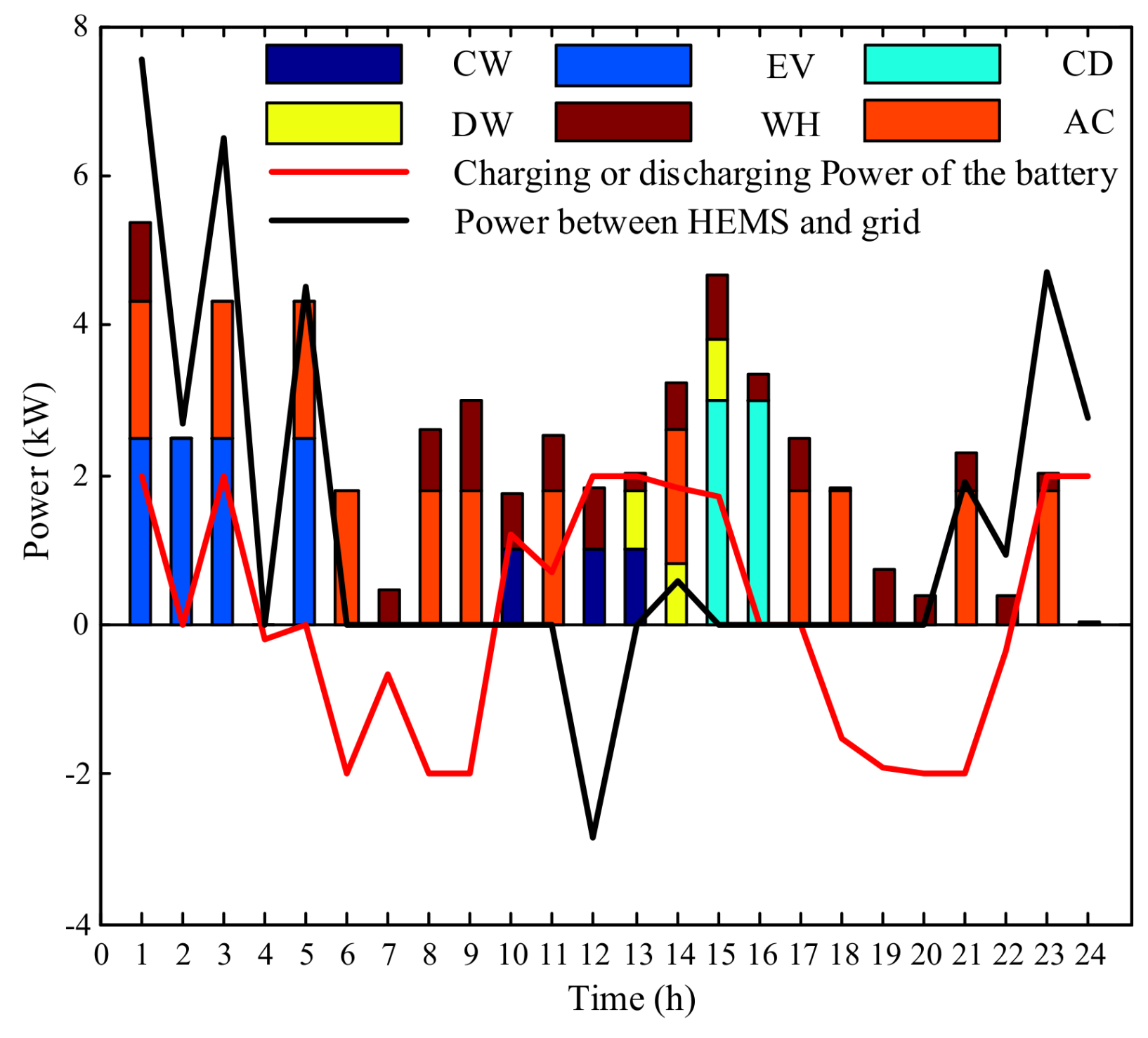
The constraints include the operational limits of household loads and the comfort requirement of customers. For a residential home, the number of appliances can reach about 15 or more. Several appliances have similar operational characteristics so they are classified into the same category. In this paper, the household loads are classified into four main categories: the loads with uncertain parameters, uncontrollable loads, uninterruptible loads, and interruptible loads. Additionally, the energy storage device can be regarded as one special load in which the active power is negative while discharging. Furthermore, because the uncontrollable loads cannot be scheduled, it is directly modeled as a fixed load curve, which will be used in the objective function to calculate the electricity bill.

2.3.1. Loads with Uncertain Parameters

The loads with uncertain parameters widely exist in houses, such as the air conditioner (AC), water heater (WH), refrigerator, etc. As stated in Section 2.1, this paper takes the AC and WH as the typical examples to be studied, which are associated the uncertainties in the outdoor temperature and hot water use.

As for an AC, due to the heat exchange between the indoor and outdoor environment, the indoor temperature is closely related to the uncertain outdoor temperature, thus being an uncertain variable as well. This relationship can be described as the following Equation (5), which is derived based on the recursive formula presented in [24]:

$$\begin{array}{l}{\tilde{\theta }}_{room,i+1}={\displaystyle \sum _{n=1}^{i}R\cdot p_{AC}^r(1-e^{\frac{-\Delta t}{RC}})}\cdot {(e^{\frac{-\Delta t}{RC}})}^{i-n}\cdot x_{AC,n}+{\displaystyle \sum _{n=1}^i(1-e^{\frac{-\Delta t}{RC}})\cdot {(e^{\frac{-\Delta t}{RC}})}^{i-n}\cdot {\tilde{\theta }}_{out,n}}\\ +{\theta }_{room,1}\cdot {(e^{\frac{-\Delta t}{RC}})}^i\begin{array}{cc}& \forall i\in \{1...N\}\end{array}\end{array}$$

(5)

where ${\tilde{\theta }}_{room,i}$ and ${\tilde{\theta }}_{out,i}$ are the uncertain indoor and outdoor temperatures at the ith time step, respectively; $x_{AC,i}$ represents the working status of the AC (0—off status, 1—heating status and −1—cooling status); the constants R and C are the equivalent heat resistance and capacity; $p_{AC}^r$ represents the rated power of the AC. It should be noted that ${\theta }_{room,1}$ is the initial indoor temperature, which is given as an initial condition before scheduling.

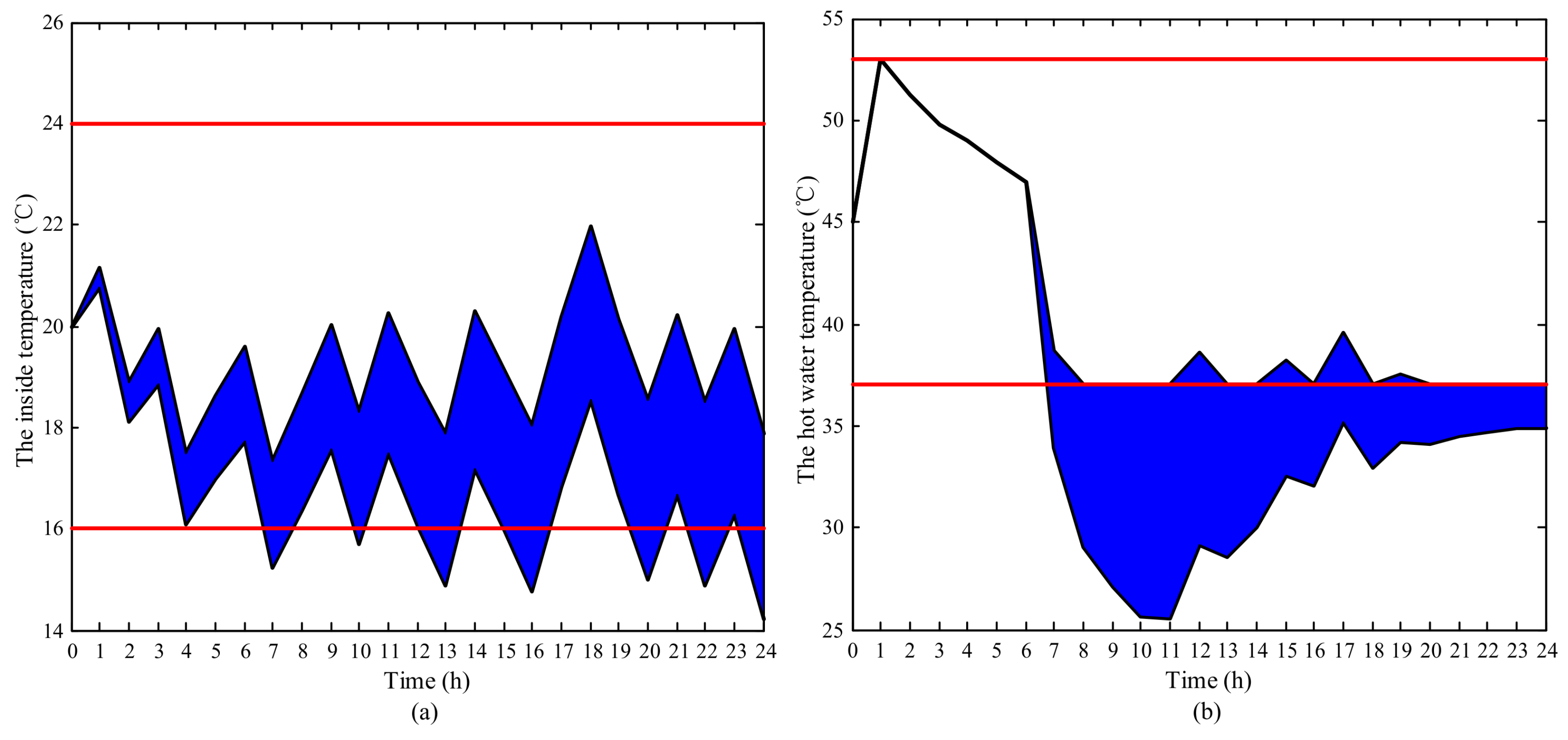
The main constraint associated with the AC is the thermal comfort constraint. That is, the uncertain indoor temperature has to be maintained in a preset range at each time step:

$${\theta }_{room}^{\min }\le {\tilde{\theta }}_{room,i+1}\le {\theta }_{room}^{\max }\begin{array}{cc}& \forall i\in \left\{1\dots N\right\}\end{array}$$

(6)

$$P_{AC,i}=\left|x_{AC,i}\right|\cdot p_{AC}^r$$

(7)

where ${\theta }_{room}^{\min }$ and ${\theta }_{room}^{\max }$ are the lower and upper boundaries of the preset comfort range. Equation (7) shows the relationship among the power consumption, the working status and the rated power of the AC.

As for a WH, the decrease of the water temperature in tank results from the heat exchange with the environment and the hot water usage. Due to the excellent insulation, the heat loss in the process of the heat exchange can be ignored [25]. Then the main cause of the temperature dropping is the hot water usage and the followed supplementary cold water. Based on the energy conservation law, the water temperature in tank can be calculated as follows:

$${\tilde{\theta }}_{water,i+1}=\{\begin{array}{l}\frac{x_{EWH,i}\cdot \rho }{CM}+(1-\frac{{\tilde{d}}_i}{M})\cdot ({\theta }_{water,1}-{\theta }_{cold})+{\theta }_{cold},i=1\\ \\ {\displaystyle \sum _{n=1}^{i-1}[{\displaystyle \prod _{k=n+1}^i(1-\frac{{\tilde{d}}_k}{M})}]\cdot \frac{x_{EWH,n}\cdot \rho }{CM}+\frac{x_{EWH,i}\cdot \rho }{CM}}+{\displaystyle \prod _{n=1}^i(1-\frac{{\tilde{d}}_n}{M})\cdot ({\theta }_{water,1}-{\theta }_{cold})+{\theta }_{cold},i=2\cdots N}\end{array}$$

(8)

where ${\tilde{\theta }}_{water,i+1}$ is the uncertain water temperature in tank at the ith time step; ${\tilde{d}}_i$ is uncertain hot water usage; $x_{EWH,i}$ is the heating power; the constant $\rho$ is the transfer coefficient between J and kWh, taking the value of 3.6 × 10⁶; the constant C is the specific heat capacity of water, being 4.2 × 10³; M is the mass of the water in full tank; and ${\theta }_{water,1}$ is the initial water temperature in tank, which is also given before scheduling.

Similar to AC, the constraint of the WH is also about thermal comfort:

$${\theta }_{water}^{\min }\le {\tilde{\theta }}_{water,i+1}\le {\theta }_{water}^{\max }\begin{array}{cc}& \forall i\in \{1...N\}\end{array}$$

(9)

$$P_{EWH,i}=x_{EWH,i}$$

(10)

where ${\theta }_{water}^{\min }$ and ${\theta }_{water}^{\max }$ are the lower and upper thresholds which are preset by customers. Equation (10) shows that the heating power of the WH is the decision variable to be optimized.

2.3.2. Interruptible Loads

Interruptible loads (IL) are allowed to be stopped during their working time so that load shifting can be achieved. Electric vehicles (EVs) and clothes washers (CWs) are two examples of this category of load. The constraints for interruptible loads can be expressed as follows:

$$x_{IL,i}=\{\begin{array}{l}0\begin{array}{cc}& \forall i\in [1,b_{IL})\cup (e_{IL},N],i\in N^{+}\end{array}\\ 0\mathrm{or}1\begin{array}{cc}\begin{array}{cc}& \end{array}& \forall i\in [b_{IL},e_{IL}],i\in N^{+}\end{array}\end{array}$$

(11)

$${\displaystyle \sum _{i=b_{IL}}^{e_{IL}}{x}_{IL,i}=l_{IL}}$$

(12)

$$P_{IL,i}=x_{IL,i}\ast p_{IL}^r$$

(13)

where $x_{IL,i}$ is the working status of interruptible loads (0—off, 1—on); $[b_{IL},e_{IL}]$ represents the allowable working period; $l_{IL}$ is the required working time to; and $p_{IL}^r$ is the rated power.

2.3.3. Uninterruptible Loads

Uninterruptible loads (UIL) have very similar operational characteristic to interruptible loads and are also allowed to be shifted. However, uninterruptible loads, like a clothes dryer (CD) or a dishwasher (DW), cannot be interrupted once it starts working. Therefore, additional constraints should be proposed [20].

$$x_{UIL,i}=\{\begin{array}{l}0\begin{array}{cc}& \forall i\in [1,b_{UIL})\cup (e_{UIL},N],i\in N^{+}\end{array}\\ 0\mathrm{or}1\begin{array}{cc}\begin{array}{cc}& \end{array}& \forall i\in [b_{UIL},e_{UIL}],i\in N^{+}\end{array}\end{array}$$

(14)

$${\displaystyle \sum _{i=b_{UIL}}^{e_{UIL}}{x}_{UIL,i}=l_{UIL}}$$

(15)

$${\displaystyle \sum _{i=j}^{j+l_{UIL}-1}{x}_{UIL,i}=(x_{UIL,j}-x_{UIL,j-1})\cdot l_{UIL}\forall j\in (b_{UIL},e_{UIL}-l_{UIL}+1],j\in N^{+}}$$

(16)

$$P_{UIL,i}=x_{UIL,i}\ast p_{UIL}^r$$

(17)

Similar to interruptible loads, $x_{UIL,i}$ is the working status of uninterruptible loads (0—off, 1—on); $[b_{UIL},e_{UIL}]$ represents the allowable working period; $l_{UIL}$ is the required working time; $p_{UIL}^r$ represents the rated power. Among the constraints, Equation (16) is the additional one for describing the uninterruptible feature.

2.3.4. Energy Storage Device

Household energy storage devices are usually batteries (e.g., lead-acid, Li-ion). Batteries charge and discharge to match the output of the local photovoltaic generation. The operational limits during the charging and discharging process are as follows [26]:

$$SO{C}_{i+1}=SO{C}_i+\frac{{\eta }_{ch}\cdot P_{ESD,i}^{ch}\cdot \Delta t}{Q_r}-\frac{P_{ESD,i}^{dch}\cdot \Delta t}{{\eta }_{dch}\cdot Q_r}-\epsilon \cdot \Delta t$$

(18)

$$0\le P_{ESD,i}^{ch}\le p_{\max }^{ch}\cdot x_{ESD,i}^{ch}\begin{array}{cc}& \forall x_{ESD,i}^{ch}\in \{0,1\}\end{array}$$

(19)

$$0\le P_{ESD,i}^{dch}\le p_{\max }^{dch}\cdot x_{ESD,i}^{dch}\begin{array}{cc}& \forall x_{ESD,i}^{dch}\in \{0,1\}\end{array}$$

(20)

$$x_{ESD,i}^{ch}+x_{ESD,i}^{dch}\le 1$$

(21)

$$SO{C}_{\min }\le SO{C}_{i+1}\le SO{C}_{\max }\begin{array}{cc}& \forall i\in \{1...N\}\end{array}$$

(22)

$$SO{C}_{N+1}\ge SO{C}_{ini}$$

(23)

where $P_{ESD,i}^{ch}$ and $P_{ESD,i}^{dch}$ represent the charging and discharging power; $x_{ESD,i}^{ch}$ and $x_{ESD,i}^{dch}$ represent the charging and discharging status ($x_{ESD,i}^{ch}$ = 1 and $x_{ESD,i}^{dch}$ = 0 indicate that the energy storage device is charging; $x_{ESD,i}^{ch}$ = 0 and $x_{ESD,i}^{dch}$ = 1 indicate that the energy storage device is discharging); ${\eta }_{ch}$ and ${\eta }_{dch}$ are the efficiency of charging and discharging; $p_{\max }^{ch}$ and $p_{\max }^{dch}$ are maximum power of charging and discharging; $\epsilon$ represents self-discharge rate; Equations (18)–(22) constrain that the battery should not overcharge and overdischarge; and Equation (23) ensures that the battery capacity at the final time step of the day is no less than that of the initial time step at the beginning of the day.

3. Robust Optimization for Household Load Scheduling

3.1. Robust Optimization

In the view of mathematics, the above scheduling problem is a mixed integer programming (MIP) problem with uncertainties. A nominal mixed integer programming is given as Equation (24).

$$\begin{array}{l}\mathrm{minimize}{\mathit{c}}^{\prime }\mathit{x}\\ \mathrm{subject}\mathrm{to}\mathit{A}\mathit{x}\le \mathit{b},\mathit{l}\le \mathit{x}\le \mathit{u}\\ x_i\in \mathbb{Z},\begin{array}{cc}& i=1,\cdots ,k\end{array}\end{array}$$

(24)

However, the existence of the uncertain parameters (some elements in $\mathit{b}$ of the Equation (24)) hinder the available methods like branch and bound method from solving the problem. Therefore, the robust optimization technique proposed by Bertsimas et al. is applied to make the uncertain programming problem solvable and to make the solutions robust.

In the robust optimization, if the element $a_{ij}$ in the matrix A is uncertain, it should be replaced by ${\tilde{a}}_{ij}$ that takes value in $\left[{\overline{a}}_{ij}-{\widehat{a}}_{ij},{\overline{a}}_{ij}+{\widehat{a}}_{ij}\right]$ of which ${\overline{a}}_{ij}$ and ${\widehat{a}}_{ij}$ are the mean value and range of the coefficient (the elements in $\mathit{b}$ can be seen as $a_{ij}$ through some transformations [12,13]). A new parameter is then defined as$z_{ij}=\left({\tilde{a}}_{ij}-{\overline{a}}_{ij}\right)/{\widehat{a}}_{ij}$, so $z_{ij}$ is a bounded random variable (but with unknown distribution) which is within [−1,1].

In order to deal with the uncertain but bounded parameters, Bertsimas et al. also introduced a number ${\Gamma }_i$ that takes value in the interval $\left[0,|J_i|\right]$, where $J_i=\left\{j|{\widehat{a}}_{ij}>0\right\}$ for each constraint. The purpose of intruding this parameter ${\Gamma }_i$ is to adjust the robustness against the level of conservatism of the solution. Specifically, the number of the coefficients that are considered as uncertain equals to $\left(\lfloor {\Gamma }_i\rfloor +1\right)$. For the former $\lfloor {\Gamma }_i\rfloor$ uncertain coefficients, the coefficients are considered to vary in the interval $\left[{\overline{a}}_{ij}-{\widehat{a}}_{ij}，{\overline{a}}_{ij}+{\widehat{a}}_{ij}\right]$; for the final uncertain coefficient, it is considered to vary in $\left[{\overline{a}}_{ij}-\left({\Gamma }_i-\lfloor {\Gamma }_i\rfloor \right){\widehat{a}}_{ij},{\overline{a}}_{ij}+\left({\Gamma }_i-\lfloor {\Gamma }_i\rfloor \right){\widehat{a}}_{ij}\right]$. The larger ${\Gamma }_i$ is, the more uncertainties will be considered during the optimization, and the more robust of the solution will be. When ${\Gamma }_i$ equals to $\left|J_i\right|$, it means that the solution can satisfy all the situations regardless of what value the uncertain parameter takes.

3.2. Robust Counterpart Transformation

Based on the above definition and method, the original programming problem Equation (24) can be transformed into the following robust counterpart [18]:

$${\displaystyle \sum _{j=1}^n{\overline{a}}_{ij}}{x}_j+\underset{z_i\in Z_i}{{\displaystyle \max }}\{{\displaystyle \sum _{j\in J_i}{\widehat{a}}_{ij}}{x}_j{z}_{ij}\}\le b_i\begin{array}{cc}& \forall i\end{array}$$

(25)

$$\mathit{l}\le \mathit{X}\le \mathit{u},Z=\{z|\left|z_{ij}\right|\le 1,\forall j\in J_i,{\displaystyle \sum _{j\in J_i}\left|z_{ij}\right|\le {\Gamma }_i}\}$$

(26)

3.2.1. Robust Counterpart Transformation of the Uncertain Outdoor Temperature

When it comes to household load scheduling, the constraints with uncertain parameters need to be transformed into the robust counterpart. Firstly, we should transform the constraints of AC into the matrix form. From the above paper, only one parameter is uncertain in each constraint and it does not appear in matrix A. Thus, introducing a new variable $x_{AC,N+1}=1$ makes this uncertain parameter classified into matrix A. To simplify the proof, set $k_1=e^{-\Delta t/RC},k_2=(1-e^{-\Delta t/RC})$. Then the matrix form for constraints is as follows:

$$\begin{array}{l}\mathit{c}\le \tilde{\mathit{A}}\cdot \left[\begin{array}{c}{x}_{AC,1}\\ x_{AC,2}\\ ⋮\\ ⋮\\ x_{AC,N}\\ x_{AC,N+1}\end{array}\right]\le \mathit{b},\tilde{\mathit{A}}=\left[\begin{array}{cccccc}{k}_2\cdot R\cdot p_{AC}^r& 0& \cdots & \cdots & 0& k_2\cdot {\tilde{\theta }}_{out,n}\\ k_2\cdot k_1\cdot R\cdot p_{AC}^r& k_2\cdot R\cdot p_{AC}^r& 0& \cdots & ⋮& {\displaystyle \sum _{n=1}^2{k}_2\cdot k_1{}^{2-n}\cdot {\tilde{\theta }}_{out,n}}\\ ⋮& ⋮& \ddots & \ddots & ⋮& ⋮\\ ⋮& ⋮& ⋮& \ddots & 0& ⋮\\ k_2\cdot k_1{}^{N-1}\cdot R\cdot p_{AC}^r& k_2\cdot k_1{}^{N-2}\cdot R\cdot p_{AC}^r& \cdots & \cdots & k_2\cdot R\cdot p_{AC}^r& {\displaystyle \sum _{n=1}^N{k}_2\cdot k_1{}^{N-n}\cdot {\tilde{\theta }}_{out,n}}\end{array}\right]\\ \mathit{b}={\left[\begin{array}{ccccc}{\theta }_{room}^{\max }-{\theta }_{room,1}\cdot k_1& {\theta }_{room}^{\max }-{\theta }_{room,1}\cdot k_1{}^2& \cdots & \cdots & {\theta }_{room}^{\max }-{\theta }_{room,1}\cdot k_1{}^N\end{array}\right]}^T\\ \mathit{c}={\left[\begin{array}{ccccc}{\theta }_{room}^{\min }-{\theta }_{room,1}\cdot k_1& {\theta }_{room}^{\min }-{\theta }_{room,1}\cdot k_1{}^2& \cdots & \cdots & {\theta }_{room}^{\min }-{\theta }_{room,1}\cdot k_1{}^N\end{array}\right]}^T\end{array}$$

(27)

Since ${\tilde{\theta }}_{out,i}\in [{\overline{\theta }}_{out,i}-{\widehat{\theta }}_{out,i},{\overline{\theta }}_{out,i}+{\widehat{\theta }}_{out,i}]$, then there exists ${\tilde{a}}_{ij}\in [{\overline{a}}_{ij}-{\widehat{a}}_{ij},{\overline{a}}_{ij}+{\widehat{a}}_{ij}],{\overline{a}}_{ij}\in \overline{\mathit{A}},{\widehat{a}}_{ij}\in \widehat{\mathit{A}}$. The details are shown in Equation (28):

$$\begin{array}{l}\overline{A}=\left[\begin{array}{cccccc}{k}_2\cdot R\cdot p_{AC}^r& 0& \cdots & \cdots & 0& k_2\cdot {\overline{\theta }}_{out,n}\\ k_2\cdot k_1\cdot R\cdot p_{AC}^r& k_2\cdot R\cdot p_{AC}^r& 0& \cdots & ⋮& {\displaystyle \sum _{n=1}^2{k}_2\cdot k_1{}^{2-n}\cdot {\overline{\theta }}_{out,n}}\\ ⋮& ⋮& \ddots & \ddots & ⋮& ⋮\\ ⋮& ⋮& ⋮& \ddots & 0& ⋮\\ k_2\cdot k_1{}^{N-1}\cdot R\cdot p_{AC}^r& k_2\cdot k_1{}^{N-2}\cdot R\cdot p_{AC}^r& \cdots & \cdots & k_2\cdot R\cdot p_{AC}^r& {\displaystyle \sum _{n=1}^N{k}_2\cdot k_1{}^{N-n}\cdot {\overline{\theta }}_{out,n}}\end{array}\right]\\ \widehat{A}=\left[\begin{array}{cccccc}0& 0& \cdots & \cdots & 0& k_2\cdot {\widehat{\theta }}_{out,n}\\ 0& 0& 0& \cdots & ⋮& {\displaystyle \sum _{n=1}^2{k}_2\cdot k_1{}^{2-n}\cdot {\widehat{\theta }}_{out,n}}\\ ⋮& ⋮& \ddots & \ddots & ⋮& ⋮\\ ⋮& ⋮& ⋮& \ddots & 0& ⋮\\ 0& 0& \cdots & \cdots & 0& {\displaystyle \sum _{n=1}^N{k}_2\cdot k_1{}^{N-n}\cdot {\widehat{\theta }}_{out,n}}\end{array}\right]\end{array}$$

(28)

Based on the robust optimization method proposed by Bertsimas, ${\Gamma }_i\in [0,\left|J_i\right|]=$[0,1] and $J_i=\{N+1\}$. Thus, the original robust counterparts from Equations (25) and (26) can be transformed into the following formulas:

$${\displaystyle \sum _{j=1}^N{\overline{a}}_{ij}}{x}_{AC,j}+\underset{z_i\in Z_i}{{\displaystyle \max }}\{{\displaystyle \sum _{j\in J_i}{\widehat{a}}_{ij}}{x}_{AC,j}{z}_{ij}\}\le b_i\begin{array}{cc}& \forall i\end{array}$$

(29)

$${\displaystyle \sum _{j=1}^N{\overline{a}}_{ij}}{x}_{AC,j}+\underset{z_i\in Z_i}{{\displaystyle \min }}\{{\displaystyle \sum _{j\in J_i}{\widehat{a}}_{ij}}{x}_{AC,j}{z}_{ij}\}\ge c_i\begin{array}{cc}& \forall i\end{array}$$

(30)

$$l\le X\le u,Z=\{z|\left|z_{ij}\right|\le 1,\forall j\in J_i,{\displaystyle \sum _{j\in J_i}\left|z_{ij}\right|\le {\Gamma }_i}\},{\Gamma }_i\in [0,1],x_{AC,N+1}=1$$

(31)

Then, going on the simply conversion of the max and min functions, the transformed formulas are:

$${\displaystyle \sum _{j=1}^N{\overline{a}}_{ij}}{x}_{AC,j}+{\displaystyle \sum _{j=\mathrm{N}+1}{\widehat{a}}_{ij}}{x}_{AC,j}{\Gamma }_i\le b_i\begin{array}{cc}& \forall i\end{array}$$

(32)

$${\displaystyle \sum _{j=1}^N{\overline{a}}_{ij}}{x}_{AC,j}+{\displaystyle \sum _{j=\mathrm{N}+1}{\widehat{a}}_{ij}}{x}_{AC,j}{\Gamma }_i\ge c_i\begin{array}{cc}& \forall i\end{array}$$

(33)

Bringing the detailed elements in Equation (28) back into Equations (32) and (33), the final linear robust counterparts can be obtained:

$$\begin{array}{l}({\displaystyle \sum _{n=1}^{i}R\cdot p_{AC}^r(1-e^{\frac{-\Delta t}{RC}})}\cdot {(e^{\frac{-\Delta t}{RC}})}^{i-n}\cdot x_{AC,n}+{\displaystyle \sum _{n=1}^i(1-e^{\frac{-\Delta t}{RC}})\cdot {(e^{\frac{-\Delta t}{RC}})}^{i-n}\cdot {\overline{\theta }}_{out,n}}+{\theta }_{room,1}\cdot {(e^{\frac{-\Delta t}{RC}})}^i\\ +{\Gamma }_{AC,i}\cdot {\displaystyle \sum _{n=1}^i(1-e^{\frac{-\Delta t}{RC}})\cdot {(e^{\frac{-\Delta t}{RC}})}^{i-n}\cdot {\widehat{\theta }}_{out,n}})\le {\theta }_{room}^{\max },\forall i\in \{1...N\}\end{array}$$

(34)

$$\begin{array}{l}({\displaystyle \sum _{n=1}^{i}R\cdot p_{AC}^r(1-e^{\frac{-\Delta t}{RC}})}\cdot {(e^{\frac{-\Delta t}{RC}})}^{i-n}\cdot x_{AC,n}+{\displaystyle \sum _{n=1}^i(1-e^{\frac{-\Delta t}{RC}})\cdot {(e^{\frac{-\Delta t}{RC}})}^{i-n}\cdot {\overline{\theta }}_{out,n}}+{\theta }_{room,1}\cdot {(e^{\frac{-\Delta t}{RC}})}^i\\ -{\Gamma }_{AC,i}\cdot {\displaystyle \sum _{n=1}^i(1-e^{\frac{-\Delta t}{RC}})\cdot {(e^{\frac{-\Delta t}{RC}})}^{i-n}\cdot {\widehat{\theta }}_{out,n}})\ge {\theta }_{room}^{\min },\forall i\in \{1...N\}\end{array}$$

(35)

where ${\Gamma }_{AC,i}$ is the parameter that control the solution robustness for the air conditioner, which takes a value in the range [0,1].

3.2.2. Robust Counterpart Transformation of Uncertain Water Demand

Similarly for the water heater, the linear robust counterparts for the constraints in Equations (8) and (9) with the uncertain water demand should be given. However, unlike the air conditioner, strong duality should be used to deduce the robust counterpart considering the multiple uncertainties (i.e., outdoor temperature and hot water use) involved. Except the uncertain parameters in matrix A, there is another one uncertain parameter which do not appear in matrix A in each constraint. Thus, introducing the new variable $x_{EWH,N+1}=1$ makes this uncertain parameter classified into matrix A. To simplify the proof, set $k=\rho /CM,r=({\theta }_{water,1}-{\theta }_{cold})>0$. Then the matrix form for constraints is as follows:

$$\begin{array}{l}c\le \tilde{A}\cdot \left[\begin{array}{c}{x}_{EWH,1}\\ x_{EWH,2}\\ ⋮\\ ⋮\\ x_{EWH,N}\\ x_{EWH,N+1}\end{array}\right]\le b,\tilde{A}=\left[\begin{array}{cccccc}k& 0& \cdots & \cdots & 0& (1-\frac{{\tilde{d}}_1}{M})\cdot r\\ k\cdot (1-\frac{{\tilde{d}}_2}{M})& k& 0& \cdots & ⋮& {\displaystyle \prod _{n=1}^2(1-\frac{{\tilde{d}}_n}{M})\cdot r}\\ ⋮& ⋮& \ddots & \ddots & ⋮& ⋮\\ ⋮& ⋮& ⋮& \ddots & 0& ⋮\\ k\cdot {\displaystyle \prod _{n=2}^N(1-\frac{{\tilde{d}}_n}{M})}& k\cdot {\displaystyle \prod _{n=3}^N(1-\frac{{\tilde{d}}_n}{M})}& \cdots & \cdots & k& {\displaystyle \prod _{n=1}^N(1-\frac{{\tilde{d}}_n}{M})\cdot r}\end{array}\right]\\ b={\left[\begin{array}{ccccc}{\theta }_{water}^{\max }-{\theta }_{cold}& {\theta }_{water}^{\max }-{\theta }_{cold}& \cdots & \cdots & {\theta }_{water}^{\max }-{\theta }_{cold}\end{array}\right]}^T\\ c={\left[\begin{array}{ccccc}{\theta }_{water}^{\min }-{\theta }_{cold}& {\theta }_{water}^{\min }-{\theta }_{cold}& \cdots & \cdots & {\theta }_{water}^{\min }-{\theta }_{cold}\end{array}\right]}^T\end{array}$$

(36)

The functions with uncertain variables in the coefficient matrix are all monotonically decreasing function, and ${\tilde{d}}_i\in [{\overline{d}}_i,{\overline{d}}_i+{\widehat{d}}_i]$. Thus, the elements in the coefficient matrix are decreasing, along with the increase of ${\tilde{d}}_i$. Thus, ${\tilde{a}}_{ij}\in [{\overline{a}}_{ij}-{\widehat{a}}_{ij},{\overline{a}}_{ij}],{\overline{a}}_{ij}\in \overline{A},{\widehat{a}}_{ij}\in \widehat{A}$ and the details are shown in Equations (37) and (38):

$$\overline{A}=\left[\begin{array}{cccccc}k& 0& \cdots & \cdots & 0& (1-\frac{{\overline{d}}_1}{M})\cdot r\\ k\cdot (1-\frac{{\overline{d}}_2}{M})& k& 0& \cdots & ⋮& {\displaystyle \prod _{n=1}^2(1-\frac{{\overline{d}}_n}{M})\cdot r}\\ ⋮& ⋮& \ddots & \ddots & ⋮& ⋮\\ ⋮& ⋮& ⋮& \ddots & 0& ⋮\\ k\cdot {\displaystyle \prod _{n=2}^N(1-\frac{{\overline{d}}_n}{M})}& k\cdot {\displaystyle \prod _{n=3}^N(1-\frac{{\overline{d}}_n}{M})}& \cdots & \cdots & k& {\displaystyle \prod _{n=1}^N(1-\frac{{\overline{d}}_n}{M})\cdot r}\end{array}\right]$$

(37)

$$\widehat{A}=\left[\begin{array}{cccccc}0& 0& \cdots & \cdots & 0& [(1-\frac{{\overline{d}}_1+{\widehat{d}}_1}{M})-(1-\frac{{\overline{d}}_1}{M})]\cdot r\\ k\cdot [(1-\frac{{\overline{d}}_2}{M})-(1-\frac{{\overline{d}}_2+{\widehat{d}}_2}{M})]& 0& 0& \cdots & ⋮& [{\displaystyle \prod _{n=2}^2(1-\frac{{\overline{d}}_n}{M})}-{\displaystyle \prod _{n=1}^2(1-\frac{{\overline{d}}_n+{\widehat{d}}_n}{M})]\cdot r}\\ ⋮& ⋮& \ddots & \ddots & ⋮& ⋮\\ ⋮& ⋮& ⋮& \ddots & 0& ⋮\\ k\cdot [{\displaystyle \prod _{n=2}^N(1-\frac{{\overline{d}}_n}{M})}-{\displaystyle \prod _{n=2}^N(1-\frac{{\overline{d}}_n+{\widehat{d}}_n}{M})]}& k\cdot [{\displaystyle \prod _{n=2}^N(1-\frac{{\overline{d}}_n}{M})}-{\displaystyle \prod _{n=3}^N(1-\frac{{\overline{d}}_n+{\widehat{d}}_n}{M})]}& \cdots & \cdots & 0& [{\displaystyle \prod _{n=2}^N(1-\frac{{\overline{d}}_n}{M})}-{\displaystyle \prod _{n=1}^N(1-\frac{{\overline{d}}_n+{\widehat{d}}_n}{M})]\cdot r}\end{array}\right]$$

(38)

Based on the robust optimization method proposed by Bertsimas, we can obtain $J_i=\{N+1\},i=1$, $J_i=\{1,\cdots ,i-1,N+1\},i=2\cdots N$ and ${\Gamma }_i\in [0,\left|J_i\right|]=$[0,i]. Thus, the original robust counterparts (25–26) can be transformed into the following formulas:

$${\displaystyle \sum _{j=1}^N{\overline{a}}_{ij}}{x}_{AC,j}+\underset{z_i\in Z_i}{{\displaystyle \max }}\{{\displaystyle \sum _{j\in J_i}{\widehat{a}}_{ij}}{x}_{AC,j}{z}_{ij}\}\le b_i\begin{array}{cc}& \forall i\end{array}$$

(39)

$${\displaystyle \sum _{j=1}^N{\overline{a}}_{ij}}{x}_{AC,j}+\underset{z_i\in Z_i}{{\displaystyle \min }}\{{\displaystyle \sum _{j\in J_i}{\widehat{a}}_{ij}}{x}_{AC,j}{z}_{ij}\}\ge c_i\begin{array}{cc}& \forall i\end{array}$$

(40)

$$l\le X\le u,Z=\{z|-1\le z_{ij}\le 0,\forall j\in J_i,{\displaystyle \sum _{j\in J_i}\left|z_{ij}\right|\le {\Gamma }_i}\},{\Gamma }_i\in [0,i],x_{AC,N+1}=1$$

(41)

Obviously, there is $\underset{z_i\in Z_i}{{\displaystyle \max }}\{{\displaystyle \sum _{j\in J_i}{\widehat{a}}_{ij}}{x}_{AC,j}{z}_{ij}\}=0$ in Equation (39). While Equation (40) cannot be directly solved which should apply the strong duality to transform. The final form of the linear robust counterparts is directly given as follows:

$${\displaystyle \sum _{j=1}^N{\overline{a}}_{ij}}{x}_{AC,j}\le b_i\begin{array}{cc}& \forall i\end{array}$$

(42)

$${\displaystyle \sum _{j=1}^N{\overline{a}}_{ij}}{x}_{AC,j}-({\Gamma }_{EWH,i}\cdot p_i+{\displaystyle \sum _{j\in J_i}{q}_{ij}})\ge c_i\begin{array}{cc}& \forall i\end{array}$$

(43)

$$p_i+q_{ij}\ge {\widehat{a}}_{ij}{y}_j\begin{array}{cc}& \forall i,\forall j\in J_i\end{array}$$

(44)

$$-y_j\le x_j\le y_j\begin{array}{cc}& \forall j\end{array}$$

(45)

$$p_i,q_{ij}\ge 0\begin{array}{cc}& \forall i,\forall j\in J_i\end{array}$$

(46)

$${\overline{a}}_{ij}\in \overline{\mathit{A}},{\widehat{a}}_{ij}\in \widehat{\mathit{A}},b_i\in \mathit{b},c_i\in \mathit{c}$$

(47)

where ${\Gamma }_{EWH,i}$ is the parameter that controls the solution robustness for the water heater, which takes a value in the range [0,i].

3.3. Solution to the Robust Counterpart

The household load scheduling with uncertain parameters is finally transformed into a mixed integer linear programming (MILP) problem. In this MILP problem, the objective function is still the one before transformation, but the constraints consist of the new constraints as presented as Equations (34)–(35), (42)–(47), and the original constraints as presented by Equations (11)–(23). Many existing methods, tools, and commercial software are available to obtain the ultimate solution. Among the abundant methods, the heuristic-based evolutionary algorithms, like particle swarm optimization (PSO), the model predictive method, and the commercial software CPLEX are some representative ones.

However, because of numerous appliances, the MILP proposed in this paper contains too many decision variables and constraints which may cause the curse of dimensionality. In this situation, the heuristic algorithms are not suitable for solving. Given the powerful calculating capacity and various solvers, this paper adopts the commercial software CPLEX (Version 12.6.3.0, IBM, New York, NY, USA, 2016) to gain the optimal schedules. CPLEX is a commercial mathematical programming solver produced by IBM Corporation in the United States. It can solve various mathematical programming problems, including linear programming (LP), quadratic programming (QP), and mixed integer linear programming (MILP) stably and efficiently.

4. Simulation Result

4.1. Simulation Design

In this paper, a day-ahead household load scheduling (from 0 a.m. to 12 p.m.) is presented. The time length of each step is set as one hour, and that is to say, the total number of time steps in the scheduling horizon is 24. The power output of the photovoltaic generation with 10 kWh capacity and the power consumption of uncontrollable loads are taken from [19], as shown in Figure 1a. The real-time price for buying electricity is easily taken from [14], shown in Figure 1b, and the price for selling electricity is assumed to be a fixed tariff, being 0.34 yuan/kWh. The operational parameters of interruptible loads, uninterruptible loads, and the energy storage device are listed in

Table 1. Parameters of interruptible loads.

Appliance	${\mathit{b}}_{\mathit{I}\mathit{L}}$	${\mathit{e}}_{\mathit{I}\mathit{L}}$	${\mathit{l}}_{\mathit{I}\mathit{L}}$ (h)	${\mathit{p}}_{\mathit{I}\mathit{L}}^{\mathit{r}}$ (KWh)
Cloth Washer (CW)	7:00	17:00	3	1
Electrical Vehicle (EV)	0:00	8:00	4	2.5

,

Table 2. Parameters of uninterruptible loads.

Appliance	${\mathit{b}}_{\mathit{U}\mathit{I}\mathit{L}}$	${\mathit{e}}_{\mathit{U}\mathit{I}\mathit{L}}$	${\mathit{l}}_{\mathit{U}\mathit{I}\mathit{L}}$ (h)	${\mathit{p}}_{\mathit{U}\mathit{I}\mathit{L}}^{\mathit{r}}$ (KWh)
Cloth Dryer (CD)	12:00	22:00	2	3
Dish Washer (DW)	12:00	20:00	3	0.8

and

Table 3. Parameters of the energy storage device.

Parameter	Value	Parameter	Value	Parameter	Value
${\eta }_{ch}$	0.95	$p_{\max }^{ch}\left(\mathrm{kW}\right)$	2	$SO{C}_{\min }$	0.1
${\eta }_{dch}$	0.95	$p_{\max }^{dch}\left(\mathrm{kW}\right)$	2	$SO{C}_{\max }$	0.9
$\epsilon (\mathrm{kWh}/\mathrm{h})$	0.004	$SO{C}_{ini}$	0.5	-	-

. Taken from [13] and [27], the heat resistance and capacity for the air conditioner are 18 °C/kW and 0.525 kWh/°C, and the mass capacity of the tank is 100 L. Additionally, the rated power of the air conditioner and water heater are 1.8 kW and 3.6 kW, respectively. The preset temperature allowable ranges as comfort constraints of the air conditioner and water heater are [16 °C, 24 °C] and [37 °C, 53 °C], respectively. Note that the air conditioner is working in the heating mode to warm the room.

According to the statistics in [17], the uncertainty set of the outdoor temperature (the possible range of the outdoor temperature) for the next day is shown in Figure 2a. As for the hot water demand, it is assumed that extra hot water usage occurs at each time step from 6 a.m. to 11 a.m., and thus the corresponding uncertainty set is assumed as shown in Figure 2b. Given the above settings, based on the theory of robust optimization, the robust parameter ${\Gamma }_{EWH,i}$ should follow:

$$\begin{array}{l}{\Gamma }_{EWH,i}\in \left\{0\right\},i\in [1,6]\\ {\Gamma }_{EWH,i}\in [0,i],i\in [7,11]\\ {\Gamma }_{EWH,i}\in [0,11],i\in [12,24]\end{array}$$

(48)

4.2. The Impact of the Uncertainties

In this subsection, the influence of the uncertainties will be analyzed. When the uncertainties in the outdoor temperature and water demand are ignored during the scheduling stage, the household load scheduling is just the result of a deterministic optimization where the average of the forecast values are used as the input parameters. Under this situation, the schedules for all appliances is shown in Figure 3. It is found that all interruptible and uninterruptible loads satisfy their corresponding constraints.

However, with executing the obtained schedules, the real temperature ranges of the air in the room and water in the tank, considering the uncertainties outdoor temperature and hot water use, are shown in Figure 4a,b, respectively. It can be seen that the actual temperature of the indoor air and hot water may take values from the blue intervals. Unfortunately, the uncertainty of the outdoor temperature generates great volatility in the indoor temperature, and at some time steps have even caused a violation of the comfort constraints (e.g., the minimum indoor temperature will reach as low as 14 °C), which are unacceptable for common customers.

Compared with the outdoor temperature, the extra hot water usage produces a more serious impact on the water temperature for the WH. As shown in Figure 4b, when the behavior of extra hot water usage happens, the water temperature immediately drops by a large degree, which is far below the lower threshold. In addition, this impact will continue until many steps after the time of extra water usage. As shown in Figure 4b, comfort violation will always happen after 7 a.m.

In summary, the uncertainties may lead to the comfort violation for both AC and WH if they are not considered during the scheduling stage. Moreover, the uncertainties may affect the optimality of schedules of other loads since they are co-scheduled in the HEMS.

4.3. Complete Robust Schedules

In order to tackle the problems caused by the uncertainties, the presented robust optimization method is used and the complete robust schedules can be obtained, under which the comfort constraints will not be violated regardless of what values the uncertain parameters take. To achieve this, all the robust parameters (Γ) in the robust optimization formulation should be taken as the maximum values. Figure 5a,b give the actual temperature ranges of the indoor air and hot water under the complete robust schedules.

Compared with Figure 4a, Figure 5a indicates that the AC turns on heating during the many periods during which the indoor temperature may be lower than the lower threshold, so that the comfort constraints are guaranteed. Additionally, compared with Figure 4b, Figure 5b shows that the water is intelligently preheated to a higher temperature during the period of 3 a.m. to 6 a.m. before the extra hot water usage. The effect of doing this is very obvious and attractive: firstly, it benefits from the low electricity price during such periods; secondly, the higher water temperature withstands the influence caused by extra hot water usage. Overall, the complete robust schedules absolutely satisfy all comfort constraints for both the AC and WH. This proves the feasibility and effectiveness of the proposed robust optimization in handling household load scheduling with uncertain parameters.

The schedules for other appliances in the complete robust schedules are shown in Figure 6. From Figure 6, it can be seen that complete robust schedules optimally rearrange all schedules and redesign the charging and discharging plans for the battery. This rescheduling leads to low electricity payment (12.75 yuan) by shifting loads to the period with low electricity prices. In spite of this, to guarantee the comfort constraints, the total electricity bill has inevitably increased by 2.94 yuan when compared with that under deterministic optimization (9.81 yuan).

4.4. Schedules with Different Robust Levels

When the robust parameter takes different values, different solutions with different levels of conservatism can be obtained. For customers, different levels of conservatism make it possible to make trade-offs between the economy and comfort. In order to compare the comfort and economy of the schedules with different robust levels, the comfort is quantitatively described by the violation rate of the comfort constraints (see [25]), which is calculated through Monte Carlo simulation where all uncertain parameters are assumed to follow uniform distribution. Without loss of generality, the robust level $\alpha$ (the ratio of the robust parameter to its maximum value), is defined to unify the levels of conservatism for all comfort constraints.

Table 4. The economy and violation rate of schedules with different robust levels.

Robust Level $\mathit{\alpha }$	Violation Rate for the Comfort Constraints of AC	Violation Rate for the Comfort Constraints of WH	Electricity Bill/Economy (Yuan)
1	0	0	12.75
0.8	0.003	0.008	12.48
0.6	0.024	0.075	12.20
0.4	0.062	0.113	11.70
0.2	0.181	0.643	11.11
0	0.517	1.000	9.81

shows the economy and comfort of the schedules with different robust levels.

As shown in Table 4, with the robust level increasing, the violation rates for the comfort constraints of the AC and WH go on declining but the electricity bill is rising. This result demonstrates that the customers can give up some comfort to save more money. Various schedules with different robust levels are offered to customers.

5. Conclusions

In this paper, the household load scheduling problem with uncertain parameters is studied. First of all, the scheduling problem is formulated as a mathematical programming problem which aims at minimizing the electricity bill under various constraints. Unlike the deterministic household load scheduling, the uncertain parameters, such as the outdoor temperature and extra hot water usage, are focused and modeled into uncertainty sets. After that, robust optimization is applied in the scheduling to deal with the uncertainties.

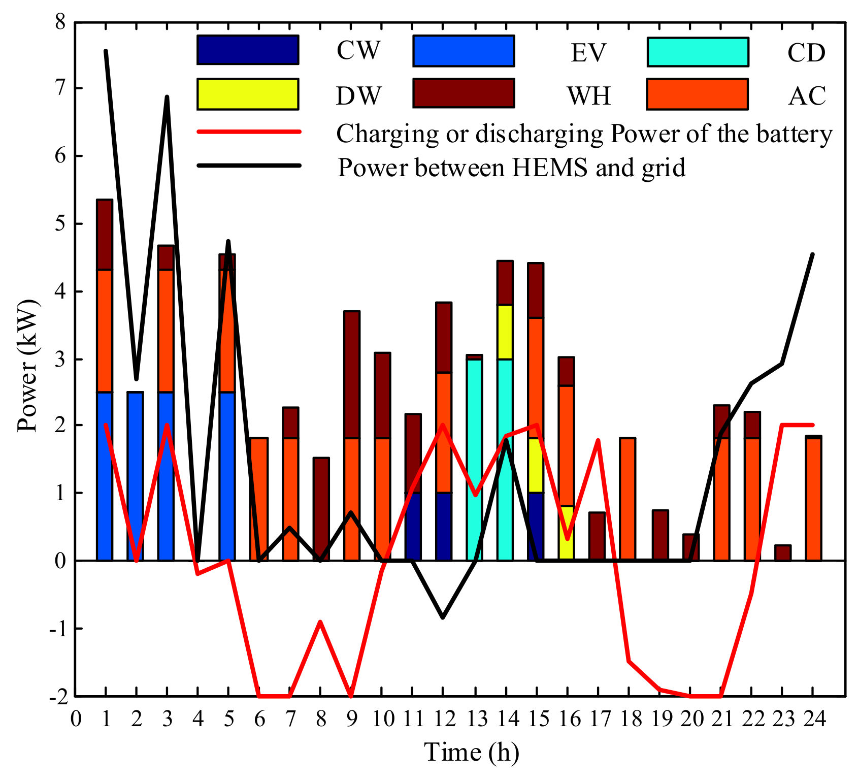
In the simulation results, the impact of uncertainties on the feasibility of the schedules is evaluated and analyzed first. The result indicates that the uncertain parameters may cause the infeasibility of the schedules derived from deterministic optimization. After that, the complete robust schedules are proposed and verified, which are capable of withstanding all the uncertainties, leading to no comfort violation. Finally, the economy and comfort of schedules with different robust levels are compared quantitatively. The proposed robust optimization method allows customers to make a trade-off between the economy and comfort, by choosing the schedules with different robust levels.

References

1. Siano, P. Demand response and smart grids—A survey. Renew. Sustain. Energy Rev. 2014, 30, 461–478. [Google Scholar] [CrossRef]
2. Datchanamoorthy, S.; Kumar, S.; Ozturk, Y.; Lee, G. Optimal time-of-use pricing for residential load control. In Proceedings of the 2011 IEEE International Conference on Smart Grid Communications, Brussels, Belgium, 17–20 October 2011; pp. 375–380. [Google Scholar]
3. Fallah, S.N.; Deo, R.C.; Shojafar, M.; Conti, M.; Shamshirband, S. Computational Intelligence Approaches for Energy Load Forecasting in Smart Energy Management Grids: State of the Art, Future Challenges, and Research Directions. Energies 2018, 11, 596. [Google Scholar] [CrossRef]
4. Beaudin, M.; Zareipour, H. Home energy management systems: A review of modelling and complexity. Renew. Sustain. Energy Rev. 2015, 45, 318–335. [Google Scholar] [CrossRef]
5. Zhao, Z.; Lee, W.C.; Shin, Y.; Song, K.B. An optimal power scheduling method for demand response in home energy management system. IEEE Trans. Smart Grid 2013, 4, 1391–1400. [Google Scholar] [CrossRef]
6. Sun, H.C.; Huang, Y.C. Optimization of power scheduling for energy management in smart homes. Procedia Eng. 2012, 38, 1822–1827. [Google Scholar] [CrossRef]
7. Paterakis, N.G.; Erdinc, O.; Bakirtzis, A.G.; Catalão, J.P. Optimal household appliances scheduling under day-ahead pricing and load-shaping demand response strategies. IEEE Trans. Ind. Inform. 2015, 11, 1509–1519. [Google Scholar] [CrossRef]
8. Liu, X.; Ivanescu, L.; Kang, R.; Maier, M. Real-time household load priority scheduling algorithm based on prediction of renewable source availability. IEEE Trans. Consum. Electron. 2012, 58, 318–326. [Google Scholar]
9. Soares, A.; Antunes, C.H.; Oliveira, C.; Gomes, Á. A multi-objective genetic approach to domestic load scheduling in an energy management system. Energy 2014, 77, 144–152. [Google Scholar] [CrossRef]
10. Bouzerdoum, M.; Mellit, A.; Pavan, A.M. A hybrid model (SARIMA–SVM) for short-term power forecasting of a small-scale grid-connected photovoltaic plant. Sol. Energy 2013, 98, 226–235. [Google Scholar] [CrossRef]
11. Weron, R. Electricity price forecasting: A review of the state-of-the-art with a look into the future. Int. J. Forecast. 2014, 30, 1030–1081. [Google Scholar] [CrossRef]
12. Chen, X.; Wei, T.; Hu, S. Uncertainty-aware household appliance scheduling considering dynamic electricity pricing in smart home. IEEE Trans. Smart Grid 2013, 4, 932–941. [Google Scholar] [CrossRef]
13. Hong, Y.Y.; Lin, J.K.; Wu, C.P.; Chuang, C.C.C. Multi-objective air-conditioning control considering fuzzy parameters using immune clonal selection programming. IEEE Trans. Smart Grid 2012, 3, 1603–1610. [Google Scholar] [CrossRef]
14. Huang, Y.; Wang, L.; Guo, W.; Kang, Q.; Wu, Q. Chance Constrained Optimization in a Home Energy Management System. IEEE Trans. Smart Grid 2016, 99, 1–9. [Google Scholar] [CrossRef]
15. Soyster, A.L. Technical note-convex programming with set-inclusive constraints and applications to inexact linear programming. Oper. Res. 1973, 21, 1154–1157. [Google Scholar] [CrossRef]
16. Ben-Tal, A.; Goryashko, A.; Guslitzer, E.; Nemirovski, A. Adjustable robust solutions of uncertain linear programs. Math. Program. 2004, 99, 351–376. [Google Scholar] [CrossRef]
17. Bertsimas, D.; Sim, M. The price of robustness. Oper. Res. 2004, 52, 35–53. [Google Scholar] [CrossRef]
18. Bertsimas, D.; Sim, M. Robust discrete optimization and network flows. Math. Program. 2003, 98, 49–71. [Google Scholar] [CrossRef]
19. Wang, C.; Zhou, Y.; Jiao, B.; Wang, Y.; Liu, W.; Wang, D. Robust optimization for load scheduling of a smart home with photovoltaic system. Energy Convers. Manag. 2015, 102, 247–257. [Google Scholar] [CrossRef]
20. Chen, Z.; Wu, L.; Fu, Y. Real-time price-based demand response management for residential appliances via stochastic optimization and robust optimization. IEEE Trans. Smart Grid 2012, 3, 1822–1831. [Google Scholar] [CrossRef]
21. Conejo, A.J.; Morales, J.M.; Baringo, L. Real-time demand response model. IEEE Trans. Smart Grid 2010, 1, 236–242. [Google Scholar] [CrossRef]
22. Wang, J.; Li, Y.; Zhou, Y. Interval number optimization for household load scheduling with uncertainty. Energy Build. 2016, 130, 613–624. [Google Scholar] [CrossRef]
23. Wang, C.; Zhou, Y.; Wu, J.; Wang, J.; Zhang, Y.; Wang, D. Robust-index method for household load scheduling considering uncertainties of customer behavior. IEEE Trans. Smart Grid 2015, 6, 1806–1818. [Google Scholar] [CrossRef]
24. Pedrasa, M.A.A.; Spooner, T.D.; MacGill, I.F. Coordinated scheduling of residential distributed energy resources to optimize smart home energy services. IEEE Trans. Smart Grid 2010, 1, 134–143. [Google Scholar] [CrossRef]
25. Du, P.; Lu, N. Appliance commitment for household load scheduling. IEEE Trans. Smart Grid 2011, 2, 411–419. [Google Scholar] [CrossRef]
26. Alrumayh, O.; Bhattacharya, K. Model predictive control based home energy management system in smart grid. In Proceedings of the 2015 IEEE Electrical Power and Energy Conference, London, ON, Canada, 26–28 October 2015; pp. 152–157. [Google Scholar]
27. 2012 ASHRAE Handbook—HVAC Systems and Equipment Amer. Soc. Heating, Refrigerating and Air-Conditioning Eng., Inc., 2012. Available online: http://app.knovel.com/web/search.v?q=2012%20ASHRA.E%20Handbook&my_subscription=FALSE&search_type=tech-reference (accessed on 10 October 2012).
Figure 1. (a) Power output of the photovoltaic generation and power consumption of the uncontrollable loads for the next day; and (b) the real-time price for the next day.
Applsci 08 00575 g001
Figure 2. (a) The uncertainty set of the outdoor temperature for the next day; and (b) the uncertainty set of the hot water demand for the next day.
Applsci 08 00575 g002
Figure 3. The schedules of household appliances (without considering the uncertainties). CW: clothes washers; EV: electric vehicles; CD: clothes dryer; DW: dishwasher; WH: water heater; AC: air conditioner.
Applsci 08 00575 g003
Figure 4. (a) The actual temperature set of the air in room; and (b) the actual temperature set of the hot water in tank.
Applsci 08 00575 g004
Figure 5. (a) The actual temperature range of the air in room (under the complete robust schedules); and (b) the actual temperature range of the hot water in tank (under the complete robust schedules).
Applsci 08 00575 g005
Figure 6. The complete robust schedules of household appliances.
Applsci 08 00575 g006