Abstract
Non-intrusive load monitoring (NILM) is a cost-effective technique for extracting device-level energy consumption information by monitoring the aggregated signal at the entrance of the electric power. With the large-scale deployment of smart metering, NILM should ideally be designed to operate purely on the low-rate data from smart meters. In this paper, an approach based on Graph Shift Quadratic Form constrained Active Power Disaggregation (GSQF-APD) is proposed, which is built upon matrix factorization and introduces graph shift quadratic form constraint according to piecewise smoothness of the power signal. In addition, a two-step iterative optimization method is designed to solve this problem. The first step minimizes the regularization term to find the signal with minimum variation, and then the second step uses the simulated annealing (SA) algorithm to iteratively minimize the objective function and constraint based on the total graph variation minimizer. Using one open-access dataset, the strength of GSQF-APD is demonstrated through three sets of experiments. The numerical results show the superior performance of GSQF-APD, with Graph Laplacian Quadratic Form constrained Active Power Disaggregation (GLQF-APD) and the state-of-the-art NILM methods as benchmarks.
1. Introduction
In recent years, the effects of global warming that are mainly caused by the increase of carbon emissions are becoming more and more tangible. Studies have demonstrated that this phenomenon is directly related to humans’ activities and their inefficient use of fossil fuel energy and natural resources, thus it is urgent to promote energy efficiency at homes, commercial sectors, and industries [1]. An effective method is to allow users to monitor the device-level energy consumption information for a long time. Indeed, statistics show that residential and commercial buildings account for 40% of total energy consumption [2], and studies have estimated that via energy feedback and specific appliance upgrade programs up to 20% of this consumption could be avoided [3].
Non-intrusive load monitoring (NILM) [4] or load disaggregation is an attractive method that decomposes the mixed energy signal into several individual signals of electrical appliances using only the measurements at the entrance of the electric power. It can provide detailed consumption information both to the energy provider and to the consumers. Compared with the conventional intrusive load monitoring technique that requires installation of one sensor for each appliance, NILM is advantageous without sub-metering or additional hardware, eliminating cost and installation complexity. Moreover, NILM can support the revamping of equipment, demand response [5], and enable the prediction of the power demand, the decision making for policy makers, and the prevention of overloading or blackouts over the energy network via appliance load shifting [6].
1.1. State of the Art in NILM
NILM appeared in the 1980s, since then, its research has been conducted for more than 30 years. Early studies in NILM aim to label the state changing event by identifying distinct electrical features of individual appliances. They can be divided into two groups, steady state and transient state analysis. The common steady-state NILM methods are based on active power and reactive power [7,8,9]. Other steady-state approaches rely on harmonics [10], voltage, and current waveform [11], or the voltage–current (V–I) trajectory analysis [12,13]. Transient analysis at start-up [14,15,16,17,18] is also a unique and effective method which can provide more distinguishable features. However, most of the aforementioned methods require high sampling frequency in the order of kHz or MHz. For example, it was suggested that the sampling rate should be at least 8 kHz for harmonics-based NILM [19]. Unfortunately, such a sampling rate is not practical in most scenarios and is especially inaccessible with the currently available smart meters.
With the large-scale deployment of smart meters in Europe, Australia, and USA [20,21], low-rate NILM based on the data captured from smart meters has drawn increasing attention. It eliminates the need to install additional acquisition devices, therefore greatly reducing hardware costs. According to the different monitoring strategies of electrical appliance operating state, low-rate NILM methods can be categorized into three main classes. The first group includes techniques for load classification, which are often referred to as event-based NILM. Its goal is to output the state transition of each appliance, such as turning on or off. The basic processing procedure of this kind of method is first detecting events, then extracting the signature related to the load event, and finally labelling step changing events via some classification algorithms. The second group comprises approaches for load disaggregation, which defines the NILM as a problem of optimization decomposition or pattern recognition. Since this type of method is not based on load event analysis, they are called non-event based NILM in general. The third group is a combination of the basic ideas in the former two methods and can be referred to as hybrid NILM [22].
Different classification tools have been used for event-based NILM. The maximum likelihood classifier used in Ref. [14] has been demonstrated to be less sensitive to power grid noise than the k-mean-based method, but this approach only works with type I appliances, i.e., the appliances with only ON/OFF states. In Ref. [23], the authors develop a systematic approach of NILM using few training examples with two generic classifiers (k-NN and naïve Bayes) for satisfactory accuracy. A method using an Artificial Neural Network (ANN) for training steady-state real power and reactive power signatures is proposed in Ref. [24], but the experiment scene is too simple, which only includes four appliances in the simulation test. In Ref. [25], the authors propose two algorithms: a low-complexity, supervised approach based on Decision Tree (DT), and an unsupervised method based on Dynamic Time Warping (DTW). Experimental results show that these two methods can disaggregate domestic loads even when the training period is very short. In order to enable correct load (i.e., class) prediction of unlabeled instances in NILM, Gillis et al. [26] introduced a co-training approach as a semi-supervised machine learning technique. However, most published event-based NILM methods make simplifying assumptions when using the labels of the events to estimate energy use for each appliance. To address this problem, Suman Giri and Mario Berges [27] present a framework for creating appliance models based on classification labels and aggregate power measurements, which can help to relax many of these assumptions. Its results show that the data-driven models outperform the heuristic models used by others.
The non-event-based NILM relies on constructing a model that includes signatures of different devices as its bases. The necessity of user intervention for creating models distinguishes unsupervised from supervised methods. The most common approaches for load disaggregation are Hidden Markov Model (HMM), an unsupervised algorithm, and its variations (see [28,29,30,31] and references therein). The early work on unsupervised NILM is presented in Ref. [28], where four different extensions of HMM are tested for better disaggregation results. However, there are some weaknesses of these algorithms, such as high computational complexity and local convergence. Recently, new methods have been proposed to address the weakness of Ref. [28], for example, Hierarchical Dirichlet Process HMM (HDP-HMM) and Hierarchical Dirichlet Process Hidden semi-Markov Model (HDP-HSMM) [31]. In order to improve the performance of standard Factorial HMM (FHMM), M. Aiad et al. [32] presented a novel energy disaggregation model that embeds the information of mutual devices interactions into the FHMM. In [33], the Hierarchical HMM (HHMM) is introduced to enhance the representation power of Markov chain based models, especially for multi-mode appliances. The aforementioned methods have been proved effective to disaggregate simple two state or multi-state loads, yet they heavily rely on clean transition from one state to another, and perform poorly for continuously varying appliances (for example, laptops or any other charger), which do not present a significant step increase in the power. On the other hand, unsupervised methods need manual adjustment of parameters, thus it is challenging to generalize them in practice. For alleviating the aforesaid problems, Kolter et al. [34] developed a method based upon a sparse coding algorithm. It uses a dictionary learning approach to construct the model of each appliance without any prior knowledge and does not make any assumptions. Motivated by the success of deep learning, a new deep learning approach, named ‘deep sparse coding’, is proposed in Ref. [35]. The characteristic is that instead of learning one level of basis/dictionary, it learns multiple layers. Moreover, in order to reduce the complexity of the training/learning process in existing decomposition based algorithms, an innovative time series distance-based approach in the temporal classification domain is proposed [36]. The main strengths are its very short and non-intrusive training period.
In this paper, we propose a low-rate hybrid NILM method. It relies on graph signal processing (GSP) theory [37], an emerging data analysis tool which can be applied to data classification by expressing the piecewise smoothness of a graph signal, and is suitable for training data that is not sufficient to establish effective classification models. Assuming that only a subset of data element labels are known, the GSP-based data classifier will predict the missing labels using the structure of the graph. The authors in Ref. [38] propose a definition of total variation on graph signals based on the concept of graph shift, which is demonstrated as useful for frequency analysis and data classification. A supervised classification method based on GSP is proposed in Ref. [39] and is applied to image and document datasets. Recently, some researchers have applied the theory of GSP into NILM, such as Ref. [40,41], yet they both adopt the graph signal’s total Laplacian smoothness as the regularization term, the classification accuracy of which is lower than that of graph shift-based regularization [38].
1.2. Contributions
Inspired by Ref. [38], we choose active power as signature and propose a GSP-based hybrid NILM algorithm. We first model the power disaggregation as a Matrix Factorization (MF) problem and formulate the objective function. Then, in order to reduce the training complexity and corresponding overhead, we integrate the technical idea of the event-based approaches into the MF problem, thus a novel hybrid NILM is formed, where GSP is used for event detection through adding constraint to the MF problem. In this paper, we construct a graph with the active power measurements and introduce the graph shift quadratic form as a new regularization term of the MF problem. Finally, we design a two-step iterative optimization method to solve the problem, the first step minimizing the regularization term to find the signal with minimum variation, and based on the total graph variation minimizer, the second step uses the simulated annealing (SA) algorithm to iteratively minimize the objective function and constraint.
We refer to the proposed algorithm in this paper as Graph Shift Quadratic Form constrained Active Power Disaggregation (GSQF-APD). The major contributions of this paper are 4-fold, which are listed as follows:
- We pose the power disaggregation as a MF problem and integrate the technical idea of the event-based approaches into the MF problem, i.e., GSQF-APD is actually a hybrid NILM, which can reduce the training complexity.
- The graph shift quadratic form is introduced as a new regularization term, which outperforms the Laplacian-based approach in classification accuracy.
- We separate the appliances from the aggregate power signal one by one in a descending order, which reduces the coverage to low power appliances, and obviously improves the disaggregation accuracy.
- Compared with other algorithms that require a training process, GSQF-APD is less dependent on training data.
2. Methodology
2.1. Problem Statement
As described previously, load disaggregation can be interpreted as a single channel source separation problem, whose main objective is to extract individual source signals from the aggregated signal taken from a single point power meter. The aggregated signal is considered to be a linear mixture of the individual sources. That is,
where P(i) is the observed mixture signal at time ti, pk(i) is the individual active power consumption of appliance k at time ti, and e(i) is the error component including random noise and some unknown appliances in the house. Additionally, Np denotes the number of all known appliances in the house.
In this paper, we use the active power variation as a signature to recover the original component signals from the mixture signal. Thus, we can rewrite the Equation (1) as,
where , , .
An effective method to deal with the source separation problem is MF, where source signal at time ti is modeled by , where denotes the bases collecting the main signatures of source and is the corresponding activation. In this paper, we adopt the difference between mean power value of appliance k’s consecutive states, , as a base. According to the above description, source signal can be expressed as,
where represents the base of device k, and is the activation coefficient.
By performing MF, we need to calculate the activation coefficient for each appliance. Assuming that is available for all appliances during training, we can formulate the corresponding optimization problem before imposing any constraints as,
In Equation (4), is an activation matrix and each row of , i.e., denotes the activation vector of appliance k. is the objective function. b is the base vector and α(i) is the activation vector of all appliances at time ti. Note that N is the total number of samples of interest and denotes the testing phase.
After activation coefficient matrix A1:Np is acquired, we can calculate the power variation of each appliance using Equation (3).
2.2. Graph Shift Quadratic Form Constrained Active Power Disaggregation
As mentioned in [42], one of the key points for designing a MF problem is to find an appropriate application-specific constraint. Unlike previous methods, in this paper, we innovatively integrate the technical idea of the event-based approaches into the MF problem. Rather, we use GSP, an emerging classification technique, to classify the active power variation at each moment by adding graph shift quadratic constraint to the optimization problem in Equation (4). According to the classification results, we can determine whether there is an appliance changing its state and obtain the activation coefficient for each device. That is to say, MF is realized. Once all activation coefficients are calculated, the power consumption at different times of each appliance can be acquired. Hence, our proposed algorithm can be called GSP-based hybrid NILM, which combines the basic ideas of event-based and non-event based NILM. In the following paragraphs, we elaborate on the GSQF-APD algorithm.
There are two basic methods to signal processing on graphs [38]. One is based on the spectral graph theory [43], adopting the graph Laplacian matrix that characterizes the underlying relational structure of the data as its fundamental building block. The other is motivated by the algebraic signal processing (ASP) theory [44,45], using the graph shift operator as its basic building block.
We construct a graph G = (v, E), where indicates the set of nodes and E is a weighted adjacency matrix of the graph. Each node vi v is associated to one sample ΔP(i), . The similarity between ΔP(i) and ΔP(j) is embodied in the edge weight between vi and vj, which is defined by the Gaussian kernel weighting function,
where σ is the scaling factor.
Using the graph, we refer to the samples as a graph signal s, where each element s(i) is indexed by node vi of the given representation graph G = (v, E). In this paper, s is defined as a set of classification labels, in which s(i) corresponds to the label of the class that element ΔP(i) belongs to. The features of a graph signal are very complex, where the smoothness is an important property to reflect the intrinsic structure of the graph signal. The smooth signal model based on the concept of smoothness is widely used in the regularization and semi-supervised learning of graphs. There are two methods to define the total smoothness on graph signals, one using the graph shift matrix (i.e., adjacency matrix) and the other via the graph Laplacian matrix.
The graph signal’s total variation (i.e., global smoothness) based on the shift matrix is defined as [38],
where is the graph shift quadratic form and is the normalized form of graph shift matrix. λmax indicates the eigenvalue of E with the largest magnitude.
The graph signal’s total variation based on the Laplacian matrix is defined as [37],
where is the graph Laplacian quadratic form. The Laplacian matrix L is defined as , where D is a diagonal matrix with elements , .
Large dataset classification usually cannot be performed manually. A common method to address the problem is to use a known structure of the dataset to predict the labels of the remaining elements [38]. In GSP-based data classification, the elements with strong correlation are usually connected by high-weight edges and represented via the same classification label s(i), which makes s vary smoothly from node to node, i.e., the signal values of connected nodes are likely to be the same [40]. Therefore, using the information about similarity between elements, we can infer unknown labels from known ones. If graph signal s is piecewise smooth with respect to the underlying graph structure, S2G(2) and S2L(2) are generally small. Thus, we can introduce them as a regularization term for the optimization problem in Equation (4). Since experiments in Ref. [38] show that classifiers designed by graph shift matrix create higher classification accuracy than the classifier based on the graph Laplacian matrix, we adopt the graph signal’s total variation based on the shift matrix as a regularization term in this paper.
In the training stage, we assume that ΔP(i) and Δpk(i) is accessible, for i = 1, …, n. The final disaggregation task is to estimate Δpk(i), for i = n + 1, …, N. First, we define an N-length graph signal sk for appliance k as,
where Thrk is the power threshold for appliance k, which is set to be one half of the base . During the training process (), if appliance k changes its state at time ti, sk(i) is set to +1; if not, sk(i) is set to −1. For the testing dataset (), we do not know whether the appliance change state at first, so we initialize sk(i) to 0.
Then, using piecewise smoothness of graph signal as a prior, we introduce S2G(2) as a regularization term of the optimization problem in Equation (4), i.e.,
where ω is a regularization parameter, which controls the relative importance of minimization Equation (4) and smoothness of graph signal.
Note that there is a mapping between sk(i) and ak(i). The following is the specific mapping process. Firstly, we need to set the classification threshold Ts. Then, if sk(i) > Ts, we can infer that appliance k changed state at time ti; otherwise, appliance k did not change state, ak(i) = 0. When judging the stat of appliance k changed at ti, we need to further determine whether it is on or off. If ΔP(i) is positive, we can judge appliance k is opening at time ti, so ak(i) = +1. On the contrary, if ΔP(i) is negative, we can judge appliance k is closing at time ti, so ak(i) = −1.
2.3. Two-Step Iterative Optimization Method
Since appliance number NP and the length of testing dataset N-n tend to be large, Equation (9) is difficult to solve as it involves a large set of optimization variables. In order to simplify the solving process, we propose a two-step iterative optimization method. The first step minimizes the regularization term to find the signal with minimum variation, and based on the total graph variation minimizer the second step iteratively minimizes both terms in Equation (9) using SA algorithm to find global optimal solution.
In Step 1, to minimize the regularization term, we adopt the following method. First, the appliances are sorted according to the average power in a descending order. Then, we separate the appliances from aggregate power signal one by one in this order until all the appliances are separated. After an appliance is disaggregated, its power consumption is removed from the total load. Note that this method reduces the coverage to low power appliances, and the disaggregation accuracy is improved obviously.
According to the above analysis, the problem of minimizing the regularization term can be transformed into solving an unconstrained quadratic optimization problem repeatedly as follows,
Let . Using the partitioned matrix computation, we can rewrite the smoothness term as,
Since has determined during training, is a constant vector, denoted by β. Thus, the Equation (10) can be simplified as,
This is a typical unconstrained quadratic optimization problem with the well-known analytical solution [46],
Once sk(n + 1:N) is determined, we can get the activation vector Ak according to the mapping between sk(i) and ak(i). Then we can calculate the power variation of appliance k according to Equation (3). After appliance k has been disaggregated, its contribution to the total power variation is removed by subtracting from , for .
We repeat the process of solving the unconstrained quadratic optimization problem for all appliances in the order of mean power from high to low. By minimizing the regularization term, we can get the optimal , for , which is also called the total graph variation minimizer.
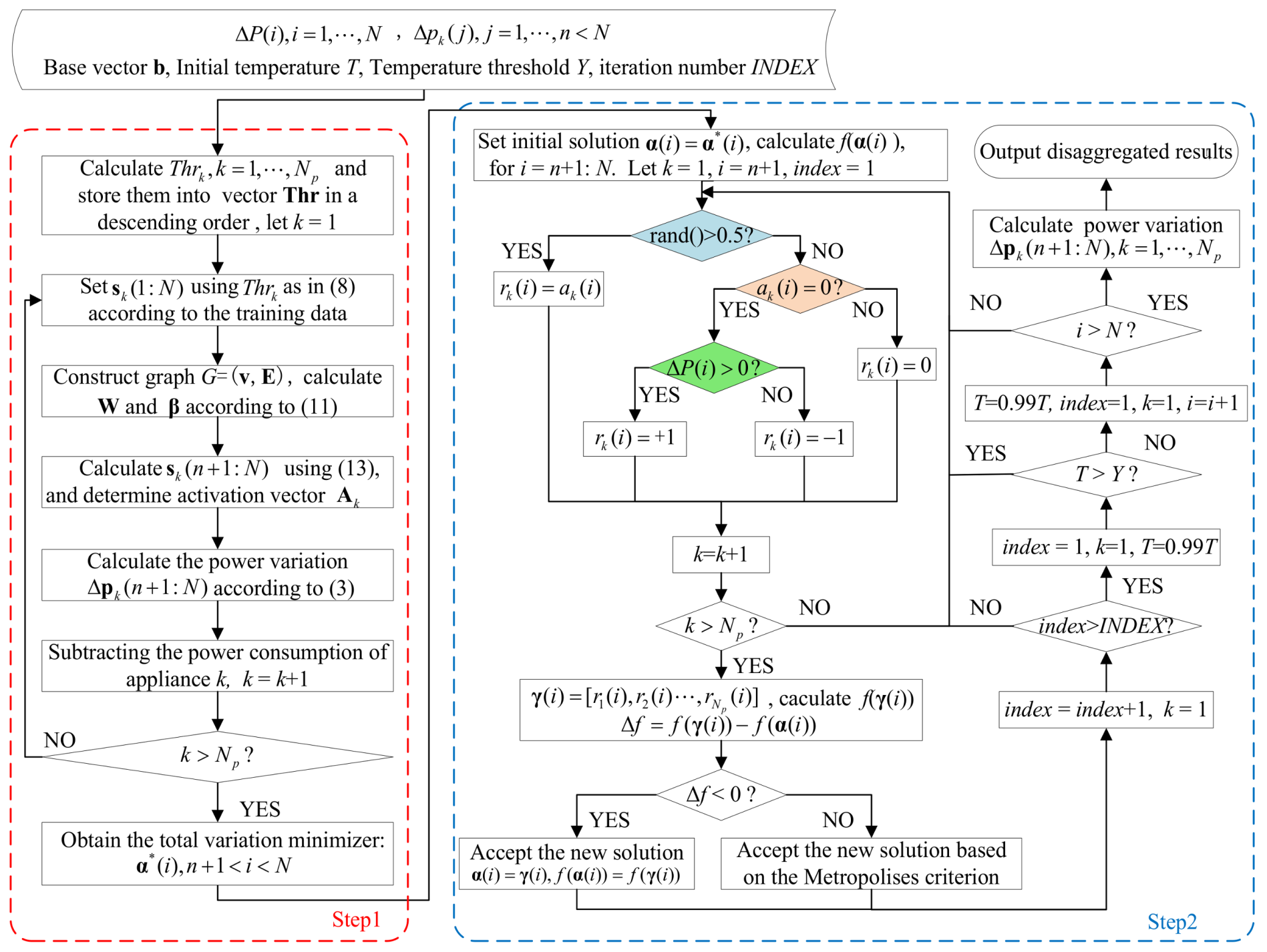
Although in Step 1 we obtain the total graph variation minimizer, it is easy to encounter the over-smooth phenomenon. In order to overcome this problem, in Step 2 we adopt the SA algorithm to minimize the objective function and constraint in Equation (9) iteratively and select the total graph variation minimizer as the initial point. In Ref. [40], the method of generating a candidate solution only guarantees to reduce the number of false positives (FP), but is unable to decrease the number of false negatives (FN). Therefore, in the two-step iterative optimization method, we make a corresponding improvement, adding the processing procedure of the FN, i.e., the green part in the Figure 1. Figure 1 shows the flow chart of the proposed GSQF-APD algorithm.
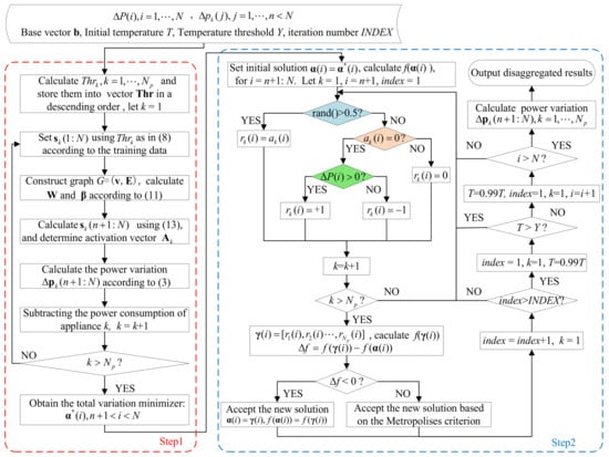
Figure 1.
Flow chart of the proposed GSQF-APD algorithm.
3. Experiment and Results
In this paper, we designed three different experiments for evaluating our proposed GSQF-APD algorithm. The first experiment is designed to demonstrate the disaggregation effectiveness of GSQF-APD. The second experiment is devised to analyze the classification accuracy of the two GSP-based methods, our proposed GSQF-APD, and the other Graph Laplacian Quadratic Form constrained Active Power Disaggregation (GLQF-APD) [40]. The third experiment is carried out to contrast the performance of the proposed algorithm with the state-of-the-art NILM approaches.
3.1. Performance Metrics
According to the research carried out in Ref. [47], the typical metrics chosen to evaluate the algorithm performance involve two aspects of the disaggregation problem: the classification of the switching activity or state transition of all appliances, and the energy disaggregation, i.e., appliances’ contribution in energy consumption.
The representative metrics to evaluate classification performance include precision (Pc), recall (Rc), F-Measure (Fc), and Accuracy (Accc) [47]. Specifically, precision is the proportion of samples recognized as class c that are correct, recall is the proportion of samples belonging to class c that are recognized correctly, F-Measure is taken to be the weighted harmonic mean of precision and recall, and accuracy is the classification ability for all samples. These metrics are defined as follows,
where c ∈ Ω, Ω denotes the set of electric appliances. TPc indicates the samples correctly labeled as ON state of class c; TNc refers to the samples correctly labeled as OFF state of class c; FPc corresponds to OFF state samples wrongly labeled as ON state of class c; FNc denotes ON state samples incorrectly labeled as OFF state of class c.
Finally, in order to present the total performance of the disaggregation system, the average classification accuracy is computed,
where Accc is the cth appliance classification accuracy.
From the perspective of energy disaggregation, the effectiveness of the algorithm is evaluated by comparing the estimated power with the ground truth power consumption.
The related metrics are defined as follows:
• Disaggregation accuracy (DA):
where is the disaggregated power consumption of appliance k at time ti; refers to the actual power of appliance k at time ti, and P(i) is the measured aggregate power consumption at time ti.
• Disaggregation error (DE):
DE provides a global comparison between the ground truth and estimated signal.
• Percentage of contribution in energy consumption (PCEC):
where PCECk represents the contribution of appliance k in energy consumption.
3.2. Experimental Results and Discussion
In this paper, the dataset used for the experiment is the REDD dataset, one open-access dataset containing detailed power usage information from US houses and specifically towards the task of energy disaggregation [48], downsampled to 1 min. For validation purposes, we treat the main type of appliance on the individual circuit as known appliance. They are: microwave (MW), dishwasher (DW), kitchen outlet (KO), stove (ST), air-conditioning (AC), washer dryer (WD), oven (OV), bathroom_gfi (BG), electronics (EL), refrigerator (REFR), and lighting (LT). Besides, baseload and unknown appliances are respectively abbreviated as BL and UN.
In order to implement a realistic energy disaggregation task and verify the effectiveness of our algorithm, the data selected for the experiment should contain all the household devices.
- (1)
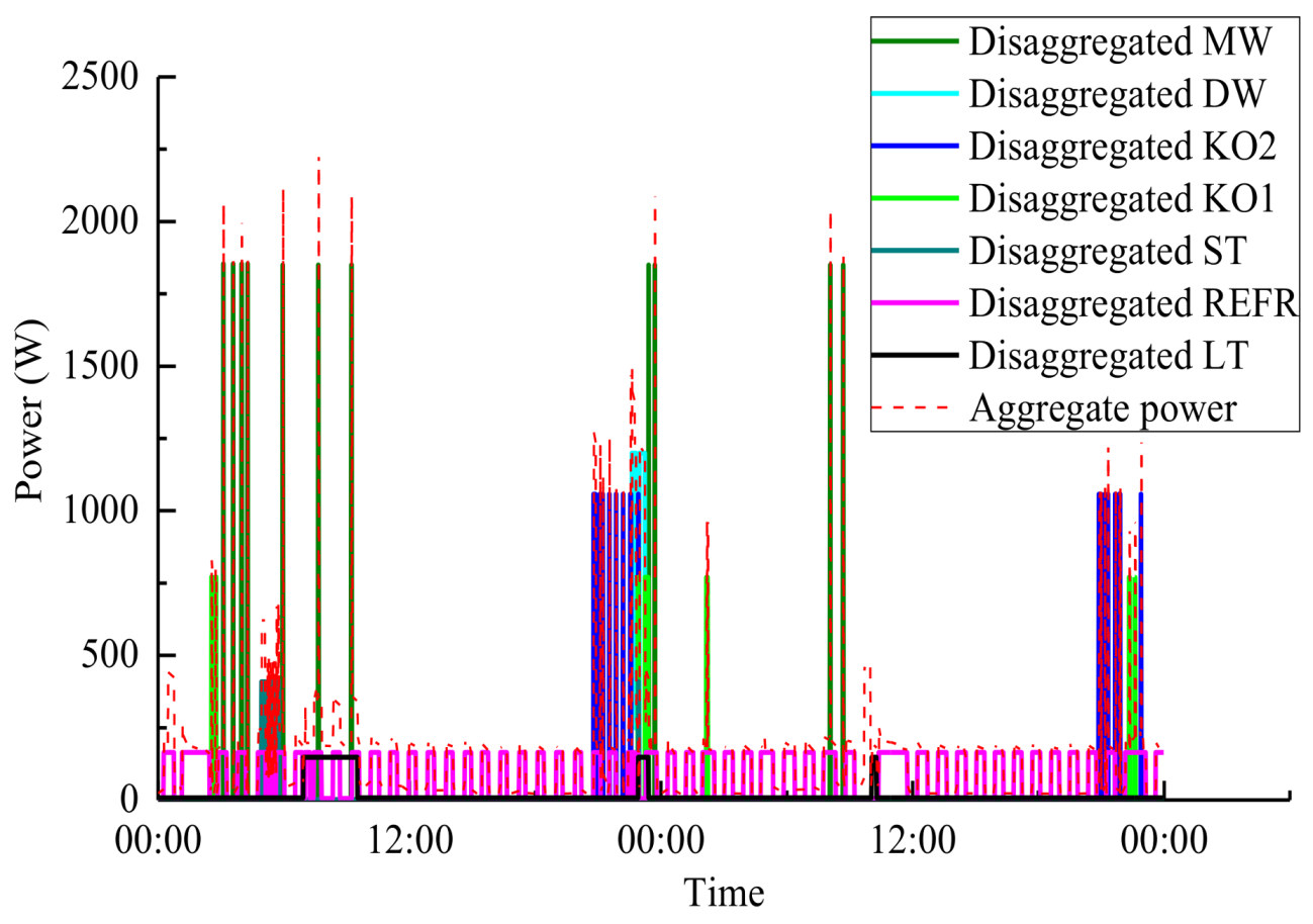
- Effectiveness of GSQF-APD algorithm. In the experiment, we use the aggregated active power readings of House 1 and House 2 from REDD dataset, and respectively select a period of time without any invalid intervals to demonstrate the disaggregation performance of the proposed algorithm. The disaggregation result of GSQF-APD for two typical days of House 2 is shown in Figure 2.
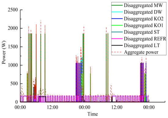 Figure 2. Disaggregation result in House 2 for two days.
The red dotted curve in Figure 2 stands for the aggregate power, and other curves indicate the estimated power consumption of each appliance, which are separated from the aggregate power through GSQF-APD algorithm. Because the aggregated power curve is the superposition of each appliance power curve; to a certain extent, the power consumption of each independent appliance will be reflected on the aggregate power curve. Note that there is a good alignment between the disaggregated results and the actual aggregate power, which demonstrates the excellent performance of GSQF-APD algorithm as a whole.
For a more detailed comparison between the ground truth and the disaggregated appliances’ active power, we conducted a further experiment using the data from House 1, which has a similar number of appliances to House 2 but presents more working states, and thus it is more challenging to disaggregate [49]. The result is shown in Figure 3. In order to evaluate the performance on a single or multiple activations, an appropriate time interval is represented in the figure for each appliance. As shown in Figure 3, the appliances with high steady powers are relatively easy to disaggregate, while those appliances with multiple working states or complex operation period are difficult to recognize. For example, the washer dryer, the oven, the bathroom_gfi, and the kitchen outlet have been successfully reconstructed, however, the microwave and the dishwasher are reconstructed with some errors. For microwave, it performs well in the activation period, whereas it brings in some false energy distribution during the off period. For dishwasher, owing to the multiple power levels, there are some working states not detected or recognized erroneously.
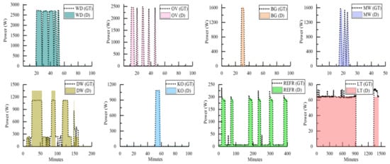
Figure 3.
Detailed disaggregation results for House 1: the disaggregated power (D) is compared against the ground truth (GT) signals.
- (2)
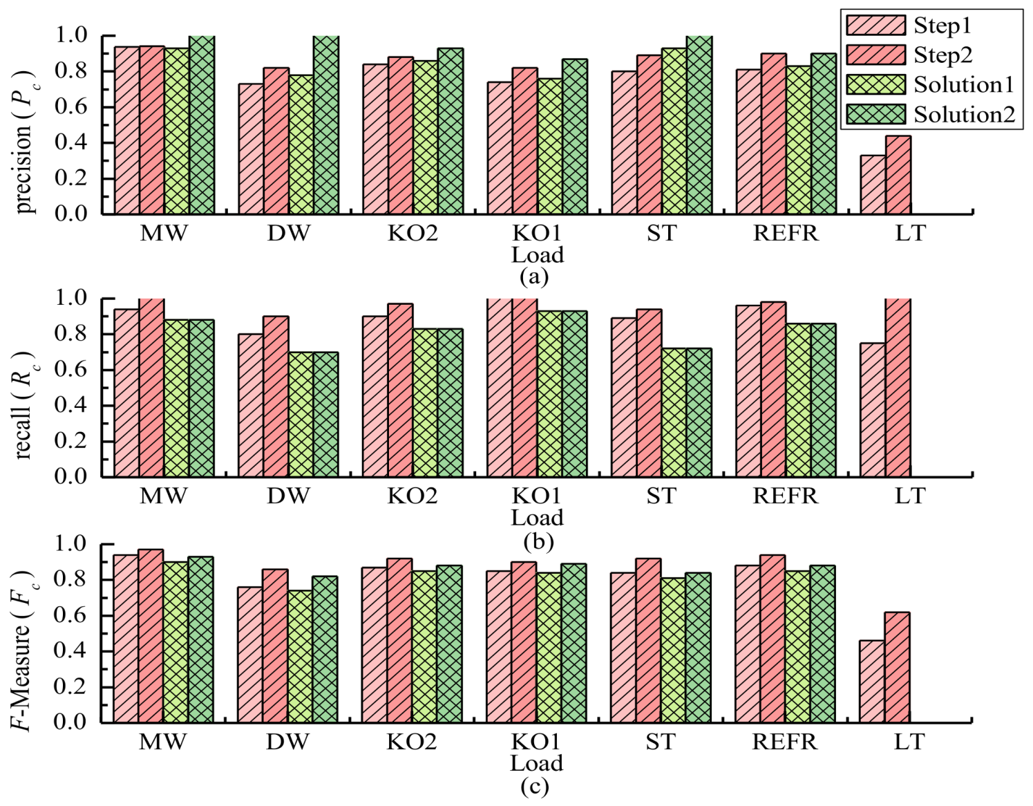
- Comparison of two GSP-based methods, GSQF-APD and GLQF-APD [40]. In this experiment, we compare the two approaches in two sections. In the first section, we compare the classification performance for House 2 of the two methods. The corresponding results are reported in Figure 4, where the precision, recall, and F-Measure are reported in Figure 4a–c, respectively. The values are related to Table 1, which is very informative about details of each appliance’s classification result and the absolute improvement of three classification metrics. Firstly, contrasting Step 1 and Step 2 of the GSQF-APD algorithm, we can see that the Step 2 performs better than Step 1 in classification accuracy, where the precision, recall, and F-measure of most appliances are significantly improved. It further illustrates that Step 2 simultaneously reduces the FP and FN events that occurred in Step 1 by using the SA algorithm to refine the results. Then, we observe that although the GLQF-APD algorithm (Solution 1 and Solution 2) produces a relatively high precision, it leads to significantly worse recall and F-measure performance than the GSQF-APD algorithm, especially for the low power appliances, for instance, lighting. In addition, note that for the GLQF-APD algorithm, the recall does not improve in Solution 2 compared with Solution 1, which indicates that the FN events are not decreased. Overall, our proposed GSQF-APD shows that average F-measure value for House 2 is 0.87, which is better than the GLQF-APD approach that shows F = 0.75 for the same house. Thus, we can conclude that the proposed method is more accurate than GLQF-APD in classification.
 Figure 4. Classification performance comparison of two GSP-based approaches for House 2. (a) Precision; (b) Recall; (c) F-Measure. Remarks: Solution 1 and Solution 2 are two approaches in Ref. [40], which are GLQF-APD.
 Table 1. Performance improvement of the proposed GSQF-APD algorithm compared with GLQF-APD.
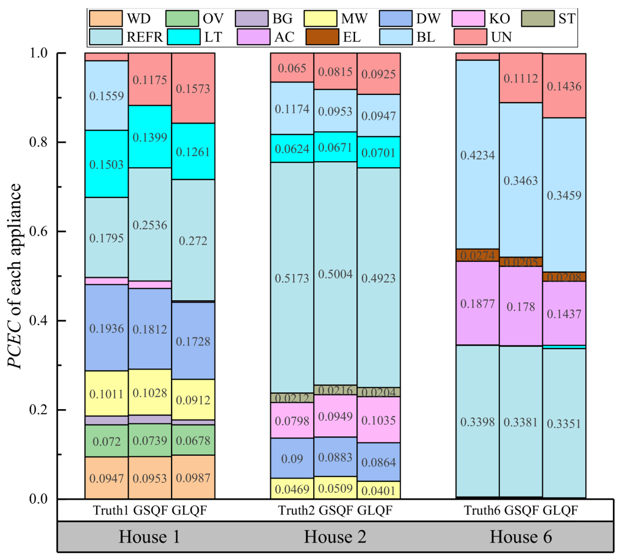
Estimating the percentage of contribution in the total energy consumption or the power usage of each appliance is also an important aspect that has received much attention. Therefore, in the second section, we analyze the PCEC value obtained by GSQF-APD and GLQF-APD. Figure 5 presents the PCEC metric of each appliance in House 1, 2 and 6 during two typical days of testing, where the left, middle, and right groups represent House 1, 2 and 6, respectively. In each group, there are three columns. The first one is the actual energy consumption contribution for each appliance in the whole home, while the last two are PCEC of all the appliances estimated by GSQF-APD and GLQF-APD. Note that baseload refers to the relatively small power produced by other devices (except the main type of appliance) on each circuit, which are characterized with constant opening over a long period of time. Unknown in the first column is defined as the difference between the measured aggregate power and the sum of the appliance’s power in each individual circuit, while in the last two columns it denotes the difference between the sum of disaggregated power and the actual aggregate consumption. From Figure 5, we find that there are some appliances not involved in the particular house. This can be attributed to three aspects: the first one is the appliance is OFF during testing, the second is the appliance’s energy consumption is too low, and the last is that the appliance is not present in the house. Analyzing the results in three houses, we observe that GSQF-APD achieves a better disaggregation performance than GLQF-APD with a closer PCEC metric to the ground truth for most appliances. In House 1, the average absolute difference after decomposition using GSQF-APD algorithm is 3.26%, whereas the average value obtained by GLQF-APD is 4.30%. Similarly, for Houses 2 and 6, the average absolute differences produced by GSQF-APD are 0.90% and 2.12%, lower than the results 1.31% and 2.97% produced by GLQF-APD, respectively.

Figure 5.
Comparison of appliance contribution to the total energy in Houses 1, 2, and 6 for GSQF-APD and GLQF-APD. Remarks: GSQF and GLQF in the figure refer to GSQF-APD and GLQF-APD, respectively.
- (3)
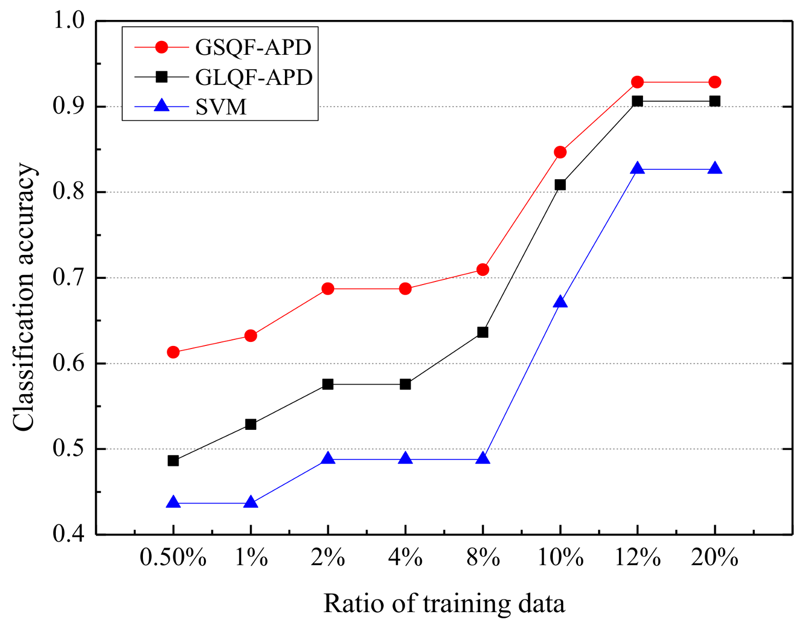
- Comparison with the state-of-the-art NILM approaches: First, a comparison of average classification accuracy of GSQF-APD with GLQF-APD and SVM-based approach for House 2 is shown in Figure 6. We can see that the two GSP-based algorithms, GSQF-APD and GLQF-APD, achieve higher accuracy than the SVM-based method, especially when the ratio of training data is small (under 8%), the difference of classification accuracy can exceed 20%. This observation demonstrates that the GSP-based approach reduces the dependence on training data compared with the SVM-based method. Furthermore, the GSQF-APD approach that uses the graph shift-based regularization term outperforms the GLQF-APD approach that introduces the Laplacian quadratic form as a regularization term. The classification accuracy gap between GSQF-APD and GLQF-APD varies from 2% to 13%. Note that the curve obtained by the SVM-based method presents a relatively obvious step-characteristic, which is due to the fact that training data in a certain interval contains the same number of useful labels.
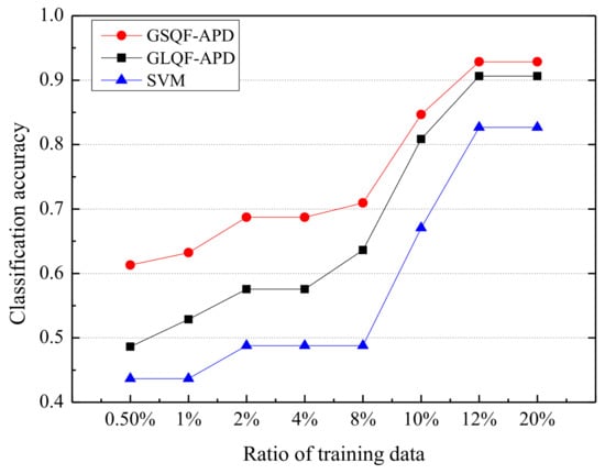 Figure 6. Classification accuracy of House 2 using GSQF-APD, GLQF-APD, and SVM algorithms.
With respect to the training complexity, we adopted the average training time as a metric. When two days of data are used, comprising over N = 2800 samples, the average training time for REDD is about 7.64 s. It is faster than the sparse coding based method which disaggregates the same amount of data in about 25 s, as reported in Ref. [35].
Then, we compare our results, FMP, with those of the GLQF-APD algorithm, FML, the HMM-based algorithm, FMH, as reported in [40], and the DT-based algorithm [25], FMDT.
Table 2, Table 3 and Table 4 show the results for REDD Houses 1, 2, 6, respectively. It can be seen that the proposed GSQF-APD approach in general outperforms other three state-of-the-art NILM approaches across all three houses. The HMM-based method has good performance in disaggregating refrigerator, since its operation is continuous and sole (i.e., usually the only one running at night) and thus has large data availability for training and facilitating good models. However, for other devices especially kitchen appliances, namely stove, microwave, and kitchen outlet, which usually have a short operation time, the HMM-based method performs poor. The DT-based method works well for the appliances that have a long operation time, such as refrigerator in the three houses and the ones that have small fluctuations in power during their steady-state operation, such as microwave in Houses 1 and 2. In addition, it is worth noting that our proposed GSQF-APD achieves the best disaggregation performance for multi-state appliances, for example washer dryer and dishwasher.
Table 2.
Performance of four low-rate NILM algorithms for House 1.
Table 3.
Performance of four low-rate NILM algorithms for House 2.
Table 4.
Performance of four low-rate NILM algorithms for House 6.
On the other hand, Table 5 presents a comparison of disaggregation accuracy of the two GSP-based methods to the three FHMM-based unsupervised methods of [31] and two FHMM-based methods of [32], as reported in [41]. As can be seen from the table, the proposed GSQF-APD algorithm provides the highest accuracy, while the other GSP-based algorithm, GLQF-APD, is more accuracy than Expectation Maximization FHMM (EM-FHMM), Factorial HDP-HMM (F-HDP-HMM) and two FHMM approaches considering or ignoring interaction, but performs more poorly than F-HDP-HSMM.
Table 5.
Disaggregation accuracy comparison with [31] and [32] for House 2.
4. Conclusions and Future Work
In this paper, a novel GSQF-APD algorithm is proposed, which is essentially a GSP-based hybrid NILM. As the experiment results show, adding the graph shift quadratic form constraint to the MF problem leads to significant improvement in classification accuracy compared with the graph Laplacian quadratic form constraint in GLQF-APD. In addition, we discuss the PCEC value of GSQF-APD and GLQF-APD using three houses power measurements from REDD dataset. The results also confirm that our method is robust with a short training phase. Moreover, we demonstrate that GSQF-APD outperforms the state-of-the-art NILM approaches, such as HMM-based algorithm, DT-based algorithm and FHMM-based algorithm. One essential limitation in power disaggregation research is the lack of a comprehensive dataset. Thus we focus on the low-rate NILM, and experiments show that our proposed algorithm works well with data sampled at a frequency of about once a minute.
Further work will include reducing computational complexity and improving event detection via pre-processing (denoising and filtering). Furthermore, we will attempt to decrease the number of FP and FN by exploiting time intervals as a feature. It may be possible to solve the problem of one state change lasting longer than the sampling duration and multiple consecutive events being identified.
Acknowledgments
This work is supported by the “Fundamental Research Funds for the Central Universities” (Project No. 2018MS001).
Author Contributions
Bing Qi and Liya Liu conceived and designed the experiments; Liya Liu performed the simulation; Liya Liu and Xin Wu analyzed the results; Liya Liu and Xin Wu wrote and revised the paper.
Conflicts of Interest
The authors declare no conflict of interest.
References
- Godina, R.; Rodrigues, E.M.G.; Pouresmaeil, E.; Matias, J.C.O.; Catalao, J.P.S. Model predictive control home energy management and optimization strategy with demand response. Appl. Sci. 2018, 8, 408. [Google Scholar] [CrossRef]
- Ariosto, T.; Memari, A.M. Comparative study of energy efficiency of glazing systems for residential and commercial buildings. In Proceedings of the Architectural Engineering Conference, State College, PA, USA, 3–5 April 2013; pp. 409–418. [Google Scholar]
- Armel, K.C.; Gupta, A.; Shrimali, G.; Albert, A. Is disaggregation the holy grail of energy efficiency? The case of electricity. Energy Policy 2013, 52, 213–234. [Google Scholar] [CrossRef]
- Hart, G.W. Nonintrusive appliance load monitoring. IEEE Proc. 1992, 80, 1870–1891. [Google Scholar] [CrossRef]
- Mocanu, E.; Nguyen, P.H.; Gibescu, M. Energy disaggregation for real-time building flexibility detection. In Proceedings of the IEEE Power and Energy Society General Meeting (PESGM), Boston, MA, USA, 17–21 July 2016. [Google Scholar]
- Abubakar, I.; Khalid, S.; Mustafa, M.; Sharee, H.; Mustapha, M. Application of load monitoring in appliances energy management—A review. Renew. Sustain. Energy Rev. 2017, 67, 235–245. [Google Scholar] [CrossRef]
- Dinesh, C.; Nettasinghe, B.W.; Godaliyadda, R.I. Residential appliance identification based on spectral information of low frequency smart meter measurements. IEEE Trans. Smart Grid 2016, 7, 2781–2792. [Google Scholar] [CrossRef]
- Figueiredo, M.; Ribeiro, B.; Almeida, A.D. Electrical signal source separation via nonnegative tensor factorization using on site measurements in a smart home. IEEE Trans. Instrum. Meas. 2014, 63, 364–373. [Google Scholar] [CrossRef]
- Xu, Y.; Milanović, J.V. Artificial-intelligence-based methodology for load disaggregation at bulk supply point. IEEE Trans. Power Syst. 2015, 30, 795–803. [Google Scholar] [CrossRef]
- Wichakool, W.; Avestruz, A.T.; Cox, R.W. Modeling and estimating current harmonics of variable electronic loads. IEEE Trans. Power Electron. 2009, 24, 2803–2811. [Google Scholar] [CrossRef]
- Wichakool, W.; Remscrim, Z.; Orji, U.A.; Leeb, S.B. Smart metering of variable power loads. IEEE Trans. Smart Grid 2015, 6, 189–198. [Google Scholar] [CrossRef]
- Hassan, T.; Javed, F.; Arshad, N. An empirical investigation of V-I trajectory based load signatures for non-intrusive load monitoring. IEEE Trans. Smart Grid 2014, 5, 870–878. [Google Scholar] [CrossRef]
- Wang, L.; Chen, X.; Wang, G. Non-intrusive load monitoring algorithm based on features of V-I trajectory. Electr. Power Syst. Res. 2018, 157, 134–144. [Google Scholar] [CrossRef]
- Henao, N.; Agbossou, K.; Kelouwani, S.; Dubé, Y.; Fournier, M. Approach in nonintrusive type I load monitoring using subtractive clustering. IEEE Trans. Smart Grid 2017, 8, 812–821. [Google Scholar] [CrossRef]
- Makonin, S.; Popowich, F.; Bajić, I.V.; Gill, B.; Bartram, L. Exploiting HMM sparsity to perform online real-time nonintrusive load monitoring. IEEE Trans. Smart Grid 2016, 7, 2575–2585. [Google Scholar] [CrossRef]
- Kong, S.; Kim, Y.; Ko, R.; Joo, S.K. Home appliance load disaggregation using cepstrum-smoothing-based method. IEEE Trans. Consum. Electron. 2015, 61, 24–30. [Google Scholar] [CrossRef]
- Chang, H.H.; Lee, M.C.; Lee, W.J.; Chien, C.L.; Chen, N. Feature extraction-based hellinger distance algorithm for nonintrusive aging load identification in residential buildings. IEEE Trans. Ind. Appl. 2016, 52, 2031–2039. [Google Scholar] [CrossRef]
- Gillis, J.M.; Chung, J.A.; Morsi, W.G. Designing new orthogonal high order wavelets for non-intrusive load monitoring. IEEE Trans. Ind. Electron. 2018, 65, 2578–2589. [Google Scholar] [CrossRef]
- Laughman, C.; Lee, K.; Cox, R.; Shaw, S.; Leeb, S.; Norford, L.; Armstrong, P. Power signature analysis. IEEE Power Energy Mag. 2003, 1, 56–63. [Google Scholar] [CrossRef]
- Department Energy Climate Change. Smart Metering Equipment Technical Specifications Version 2; UK Government: London, UK, 2013.
- Elburg, H.V. Dutch Energy Savings Monitor for the Smart Meter; Rijksdienst Voor Ondernemend Nederland: Assen, The Netherland, 2014. [Google Scholar]
- Liang, J.; Ng, S.K.K.; Kendall, G.; Cheng, J.W.M. Load signature study-part I: Basic concept, structure, and methodology. IEEE Trans. Power Deliv. 2010, 25, 551–560. [Google Scholar] [CrossRef]
- Yang, C.C.; Soh, C.S.; Yap, V.V. A systematic approach in appliance disaggregation using k-nearest neighbours and naive Bayes classifiers for energy efficiency. Energy Effic. 2018, 11, 239–259. [Google Scholar] [CrossRef]
- Biansoongnern, S.; Plangklang, B. Nonintrusive load monitoring (NILM) using an Artificial Neural Network in embedded system with low sampling rate. In Proceedings of the 13th International Conference on Electrical Engineering/Electronics, Computer, Telecommunications and Information Technology (ECTI-CON), Chiang Mai, Thailand, 28 June–1 July 2016; pp. 1–4. [Google Scholar]
- Liao, J.; Elafoudi, G.; Stankovic, L.; Stankovic, V. Non-intrusive appliance load monitoring using low-resolution smart meter data. In Proceedings of the IEEE International Conference on Smart Grid Communications (SmartGridComm), Venice, Italy, 3–6 November 2014; pp. 535–540. [Google Scholar]
- Gillis, J.M.; Morsi, W.G. Non-intrusive load monitoring using semi-supervised machine learning and wavelet design. IEEE Trans Smart Grid 2017, 8, 2648–2655. [Google Scholar] [CrossRef]
- Giri, S.; Berges, M. An energy estimation framework for event-based methods in Non-Intrusive Load Monitoring. Energy Convers. Manag. 2015, 90, 488–498. [Google Scholar] [CrossRef]
- Kim, H.; Marwah, M.; Arlitt, M.; Lyon, G.; Han, J. Unsupervised disaggregation of low frequency power measurements. In Proceedings of the 11th SIAM International Conference on Data Mining, Mesa, AZ, USA, 28–30 April 2011; pp. 747–758. [Google Scholar]
- Parson, O.; Ghosh, S.; Weal, M.; Rogers, A. An unsupervised training method for nonintrusive appliance load monitoring. Artif. Intell. 2014, 217, 1–19. [Google Scholar] [CrossRef]
- Bonfigli, R.; Principi, E.; Fagiani, M. Non-intrusive load monitoring by using active and reactive power in additive Factorial Hidden Markov Models. Appl. Energy 2017, 208, 1590–1607. [Google Scholar] [CrossRef]
- Johnson, M.J.; Willsky, A.S. Bayesian nonparametric hidden semi-Markov models. J. Mach. Learn. Res. 2013, 14, 673–701. [Google Scholar]
- Aiad, M.; Peng, H.L. Unsupervised approach for load disaggregation with devices interactions. Energy Build. 2016, 116, 96–103. [Google Scholar] [CrossRef]
- Kong, W.; Dong, Z.Y.; Hill, D.J. A hierarchical hidden Markov model framework for home appliance modelling. IEEE Trans. Smart Grid 2016. [Google Scholar] [CrossRef]
- Kolter, J.Z.; Batra, S.; Ng, A.Y. Energy disaggregation via discriminative sparse coding. In Proceedings of the 24th Annual Conference on Neural Information Processing Systems, Vancouver, BC, Canada, 6–9 December 2010; pp. 1153–1161. [Google Scholar]
- Singh, S.; Majumdar, A. Deep sparse coding for non-intrusive load monitoring. IEEE Trans. Smart Grid 2017. [Google Scholar] [CrossRef]
- Basu, K.; Debusschere, V.; Douzal-Chouakria, A. Time series distance-based methods for non-intrusive load monitoring in residential buildings. Energy Build. 2015, 96, 109–117. [Google Scholar] [CrossRef]
- Shuman, D.I.; Narang, S.K.; Frossard, P. The emerging field of signal processing on graphs: Extending high-dimensional data analysis to networks and other irregular domains. IEEE Signal Process. Mag. 2013, 30, 83–98. [Google Scholar] [CrossRef]
- Sandryhaila, A.; Moura, J.M.F. Discrete signal processing on graphs: Frequency analysis. IEEE Trans. Signal Process. 2014, 62, 3042–3054. [Google Scholar]
- Sandryhaila, A.; Moura, J. Classification via regularization on graphs. In Proceedings of the IEEE Global Conference on Signal and Information Processing (GlobalSIP), Austin, TX, USA, 3–5 December 2013; pp. 495–498. [Google Scholar]
- He, K.; Stankovic, L.; Liao, J. Non-intrusive load disaggregation using graph signal processing. IEEE Trans. Smart Grid 2016. [Google Scholar] [CrossRef]
- Zhao, B.; Stankovic, L.; Stankovic, V. On a training-less solution for non-intrusive appliance load monitoring using graph signal processing. IEEE Access 2016, 4, 1784–1799. [Google Scholar] [CrossRef]
- Rahimpour, A.; Qi, H.; Fugate, D. Non-intrusive energy disaggregation using non-negative matrix factorization with sum-to-k constraint. IEEE Trans. Power Syst. 2017, 32, 4430–4441. [Google Scholar] [CrossRef]
- Chung, F.R.K. Spectral Graph Theory; American Mathematical Society (AMS): Providence, RI, USA, 1996. [Google Scholar]
- Püschel, M.; Moura, J.M.F. Algebraic signal processing theory: Foundation and 1-D time. IEEE Trans. Signal Process. 2008, 56, 3572–3585. [Google Scholar] [CrossRef]
- Püschel, M.; Moura, J.M.F. Algebraic signal processing theory: 1-D space. IEEE Trans. Signal Process. 2008, 56, 3586–3599. [Google Scholar] [CrossRef]
- Boyd, S.; Vandenberghe, L. Quadratic optimization problems. In Convex Optimization; Cambridge University Press: New York, NY, USA, 2009; pp. 166–170. [Google Scholar]
- Bonfigli, R.; Squartini, S.; Fagiani, M.; Piazza, F. Unsupervised algorithms for non-intrusive load monitoring: An up-to-date overview. In Proceedings of the IEEE 15th International Conference on Environment and Electrical Engineering (EEEIC), Rome, Italy, 10–13 June 2015; pp. 1175–1180. [Google Scholar]
- Kolter, J.; Johnson, M. REDD: A public data set for energy disaggregation research. In Proceedings of the Workshop on Data Mining Applications in Sustainability, San Diego, CA, USA, 21–24 August 2011; pp. 1–6. [Google Scholar]
- Egarter, D.; Pöchacker, M.; Elmenreich, W. Complexity of power draws for load disaggregation. Comput. Sci. 2015, arXiv:1501.02954. [Google Scholar]

© 2018 by the authors. Licensee MDPI, Basel, Switzerland. This article is an open access article distributed under the terms and conditions of the Creative Commons Attribution (CC BY) license (http://creativecommons.org/licenses/by/4.0/).