Damage Imaging in Lamb Wave-Based Inspection of Adhesive Joints


Abstract
:1. Introduction
2. Materials and Methods
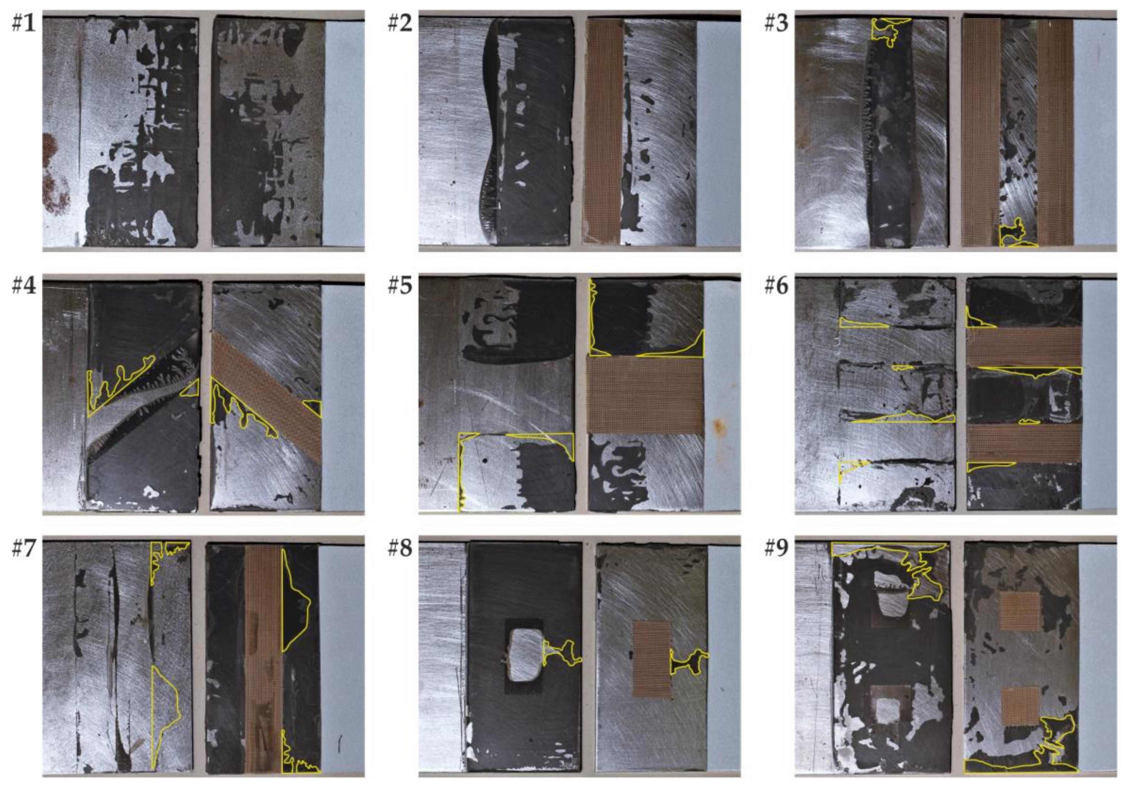
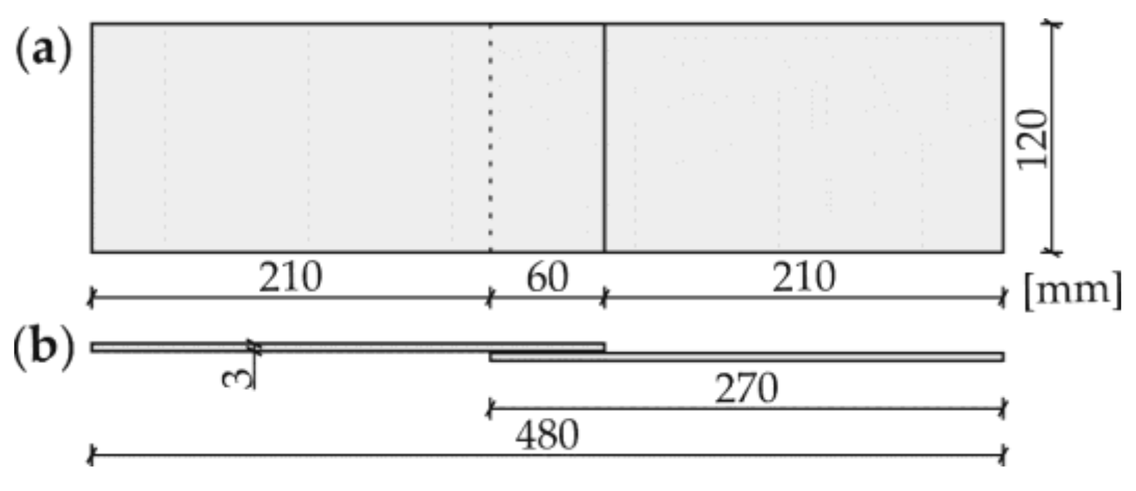
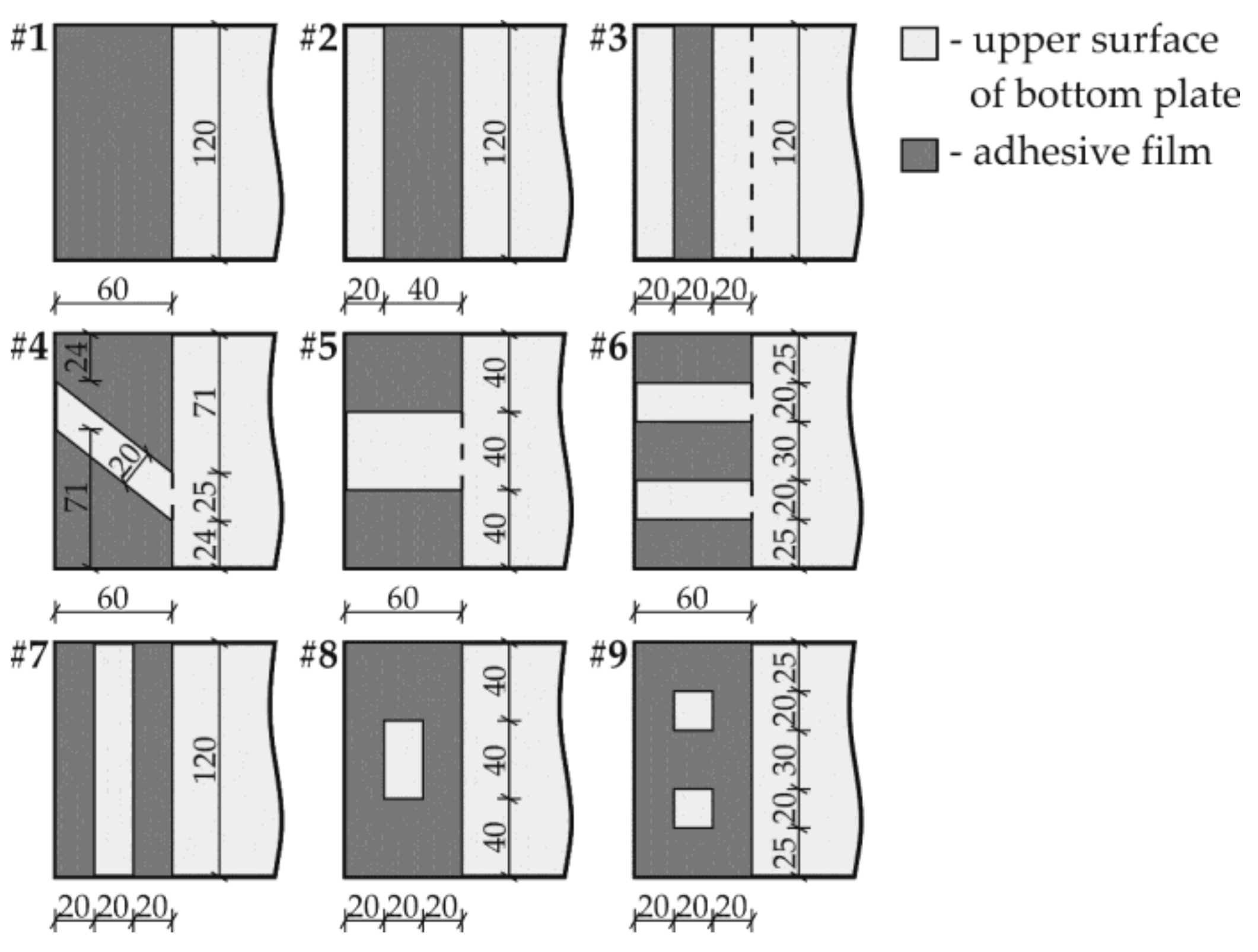
2.1. Description of Specimens
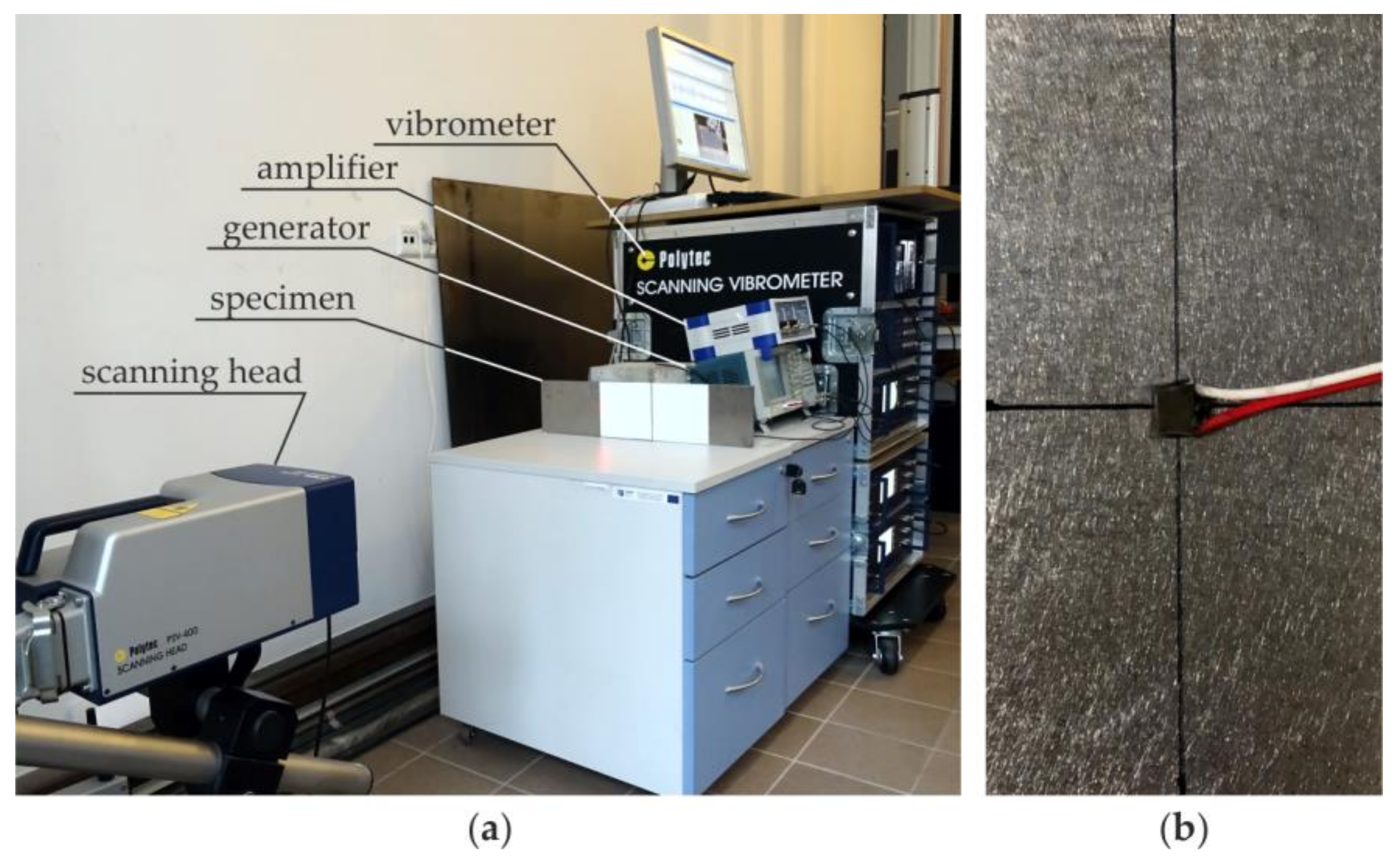
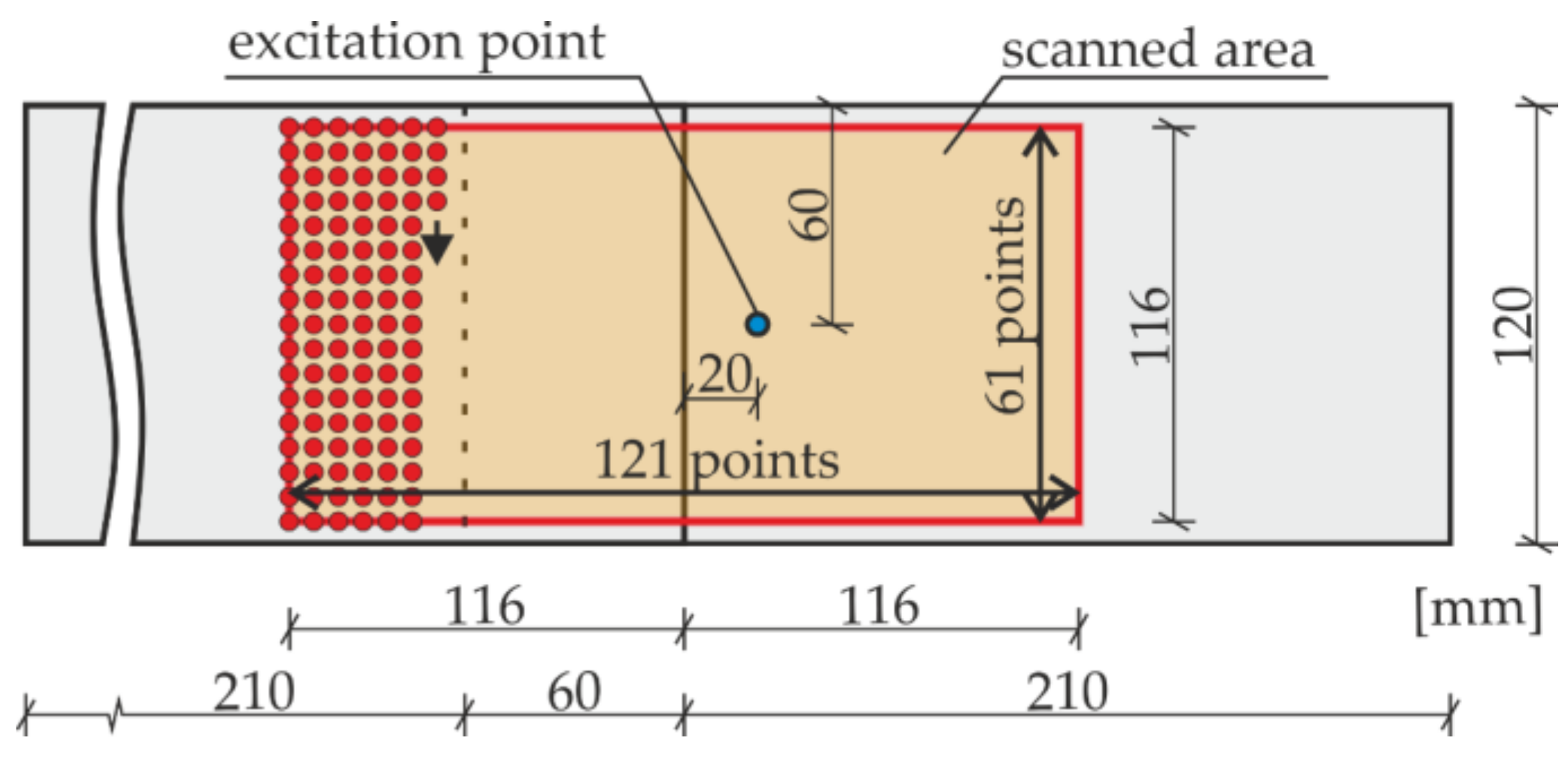
2.2. Experimental Setup
2.3. Weighted Root Mean Square Damage Imaging
3. Results and Discussion
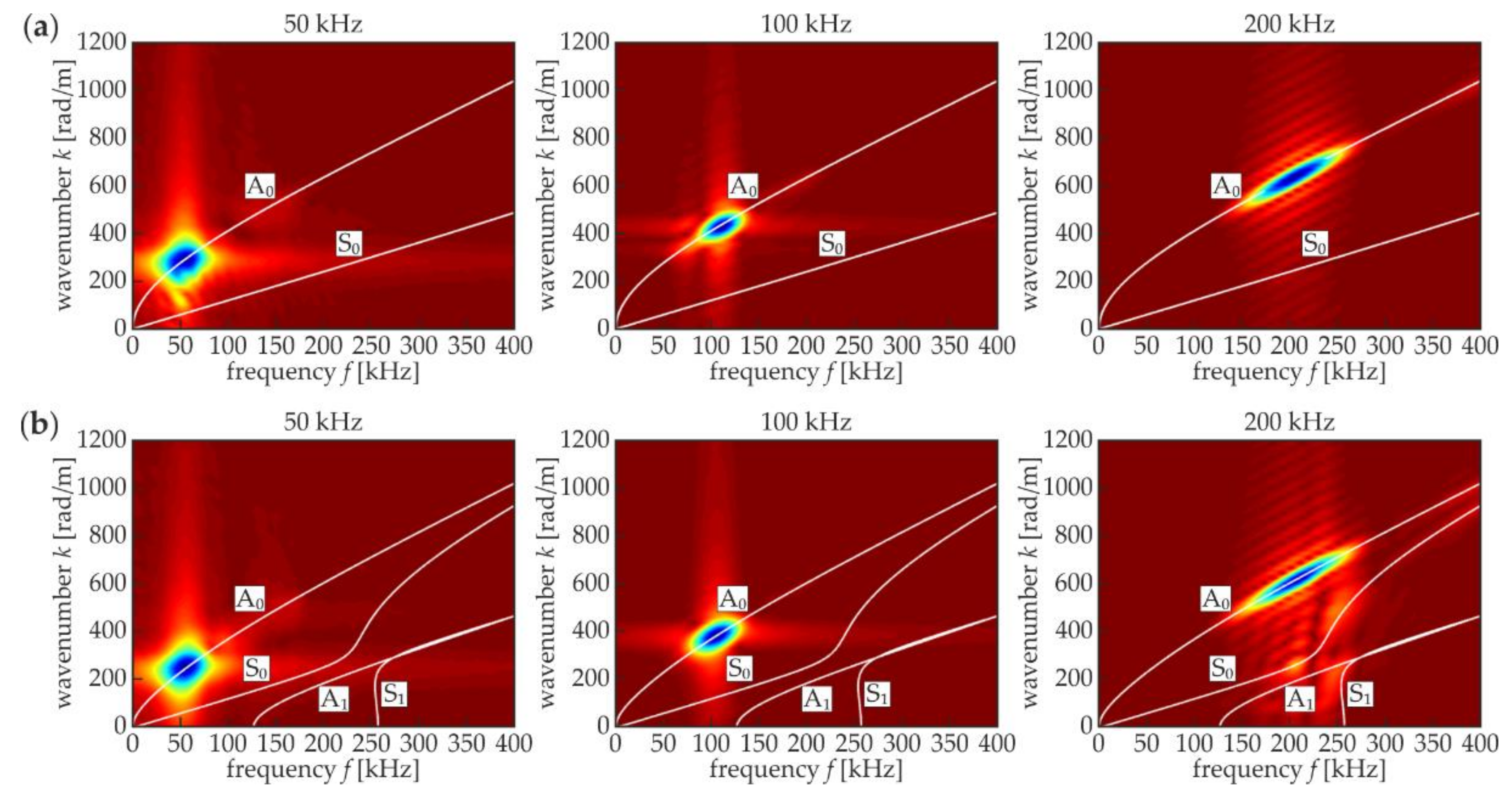
3.1. Dispersion Curves
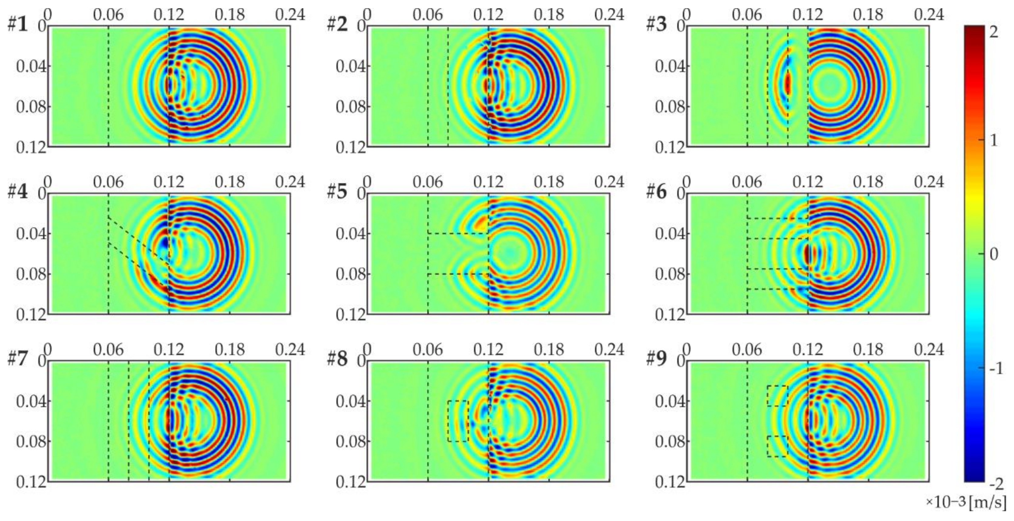
3.2. SLDV Maps
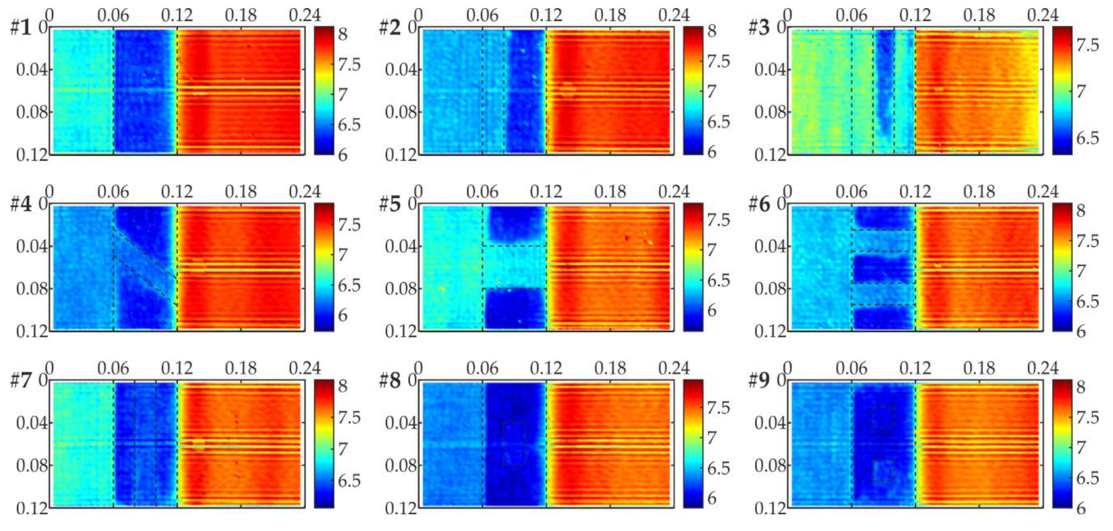
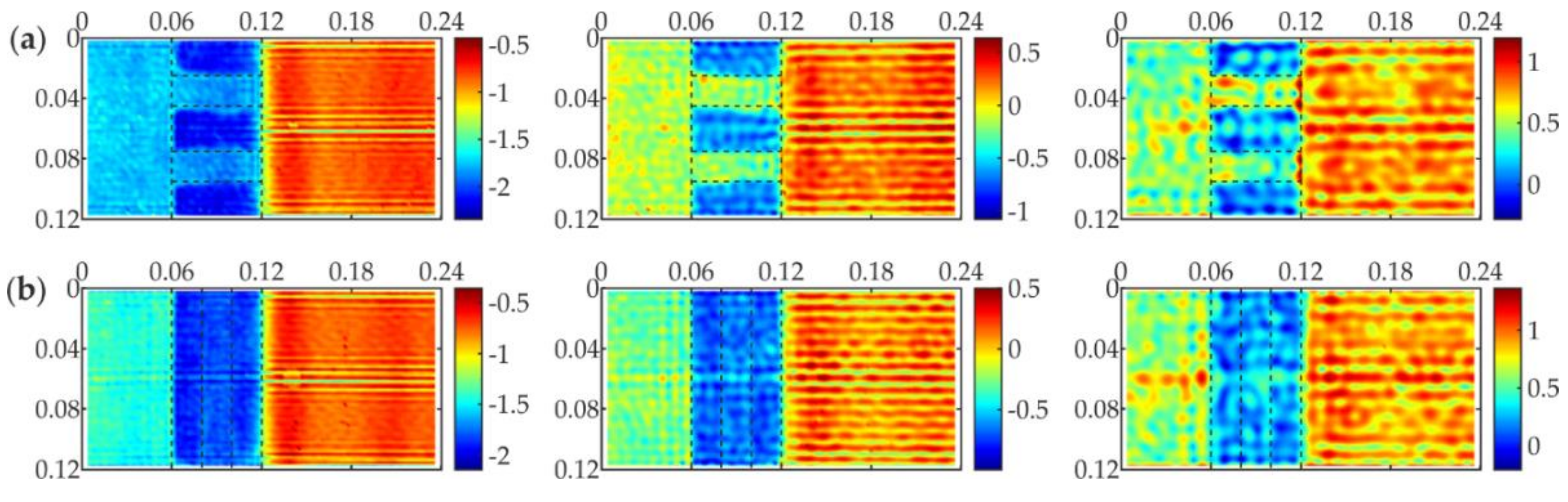
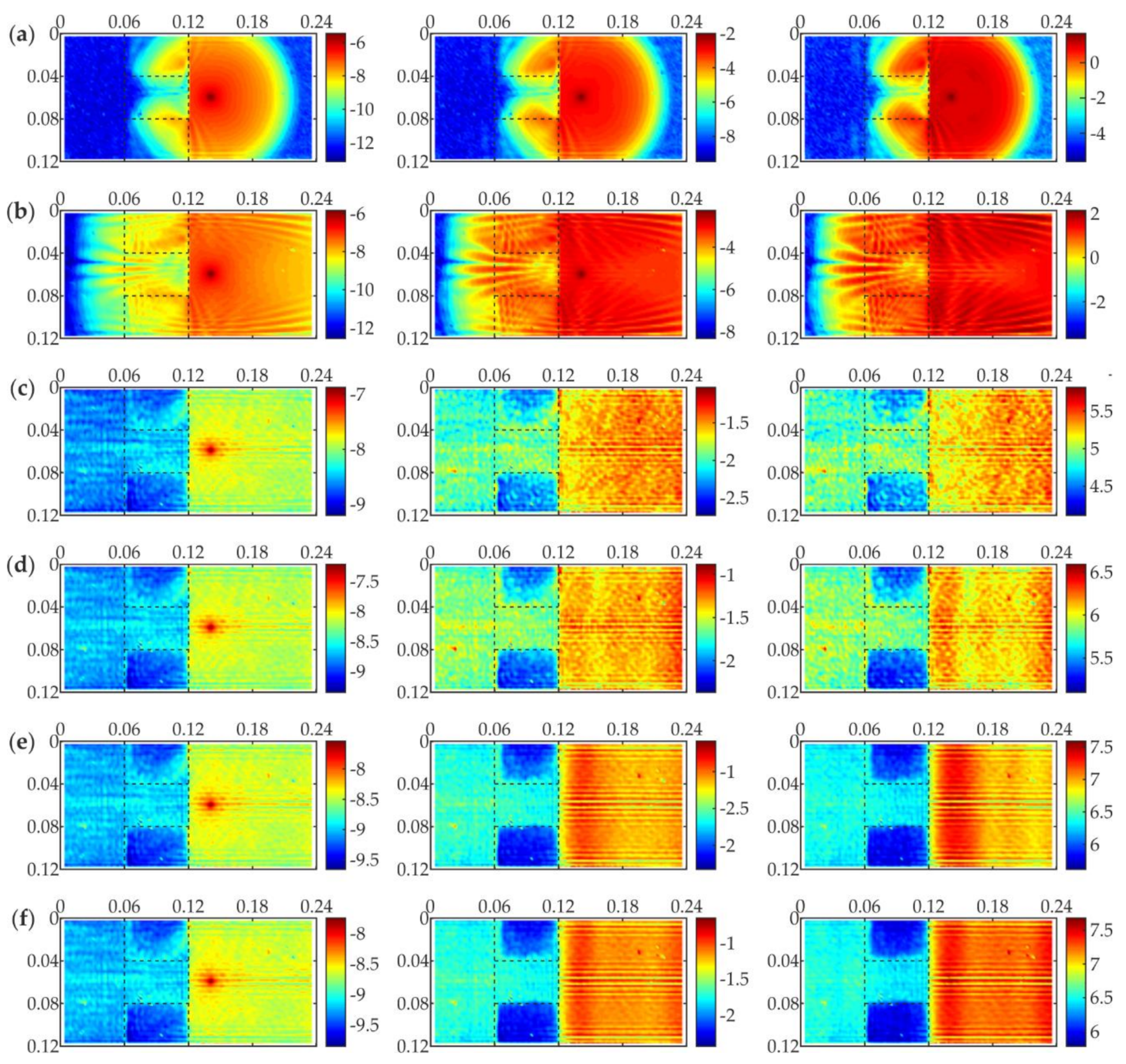
3.3. WRMS Imaging
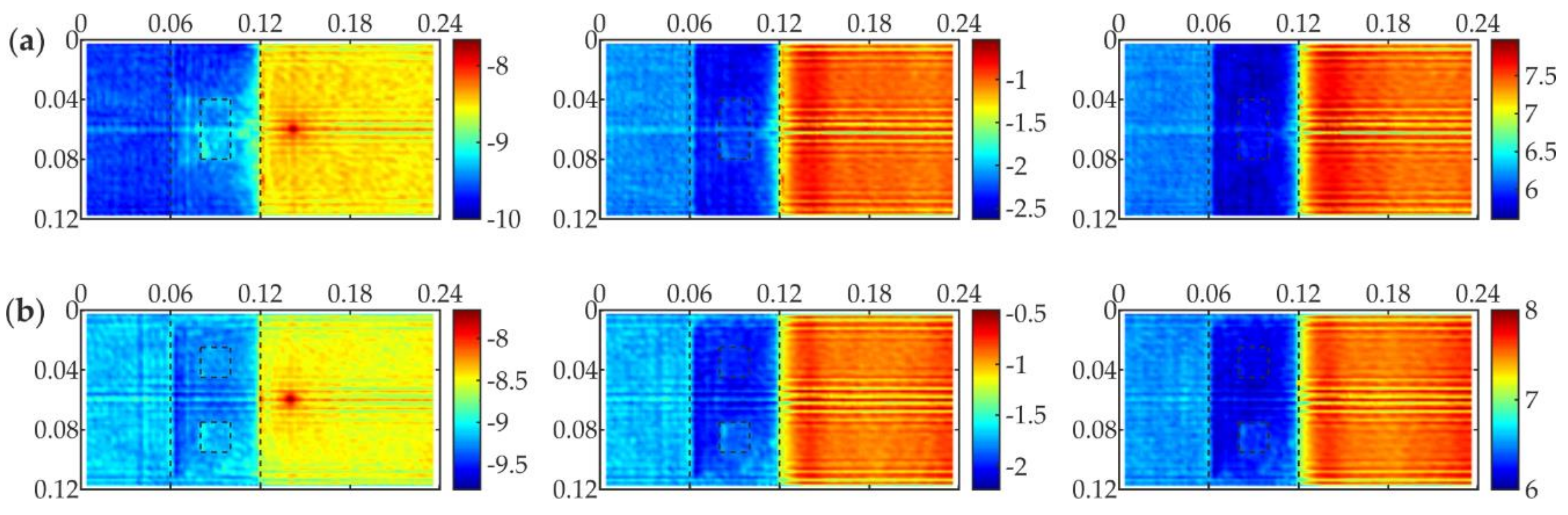
3.3.1. Influence of Time Window and Weighting Factor
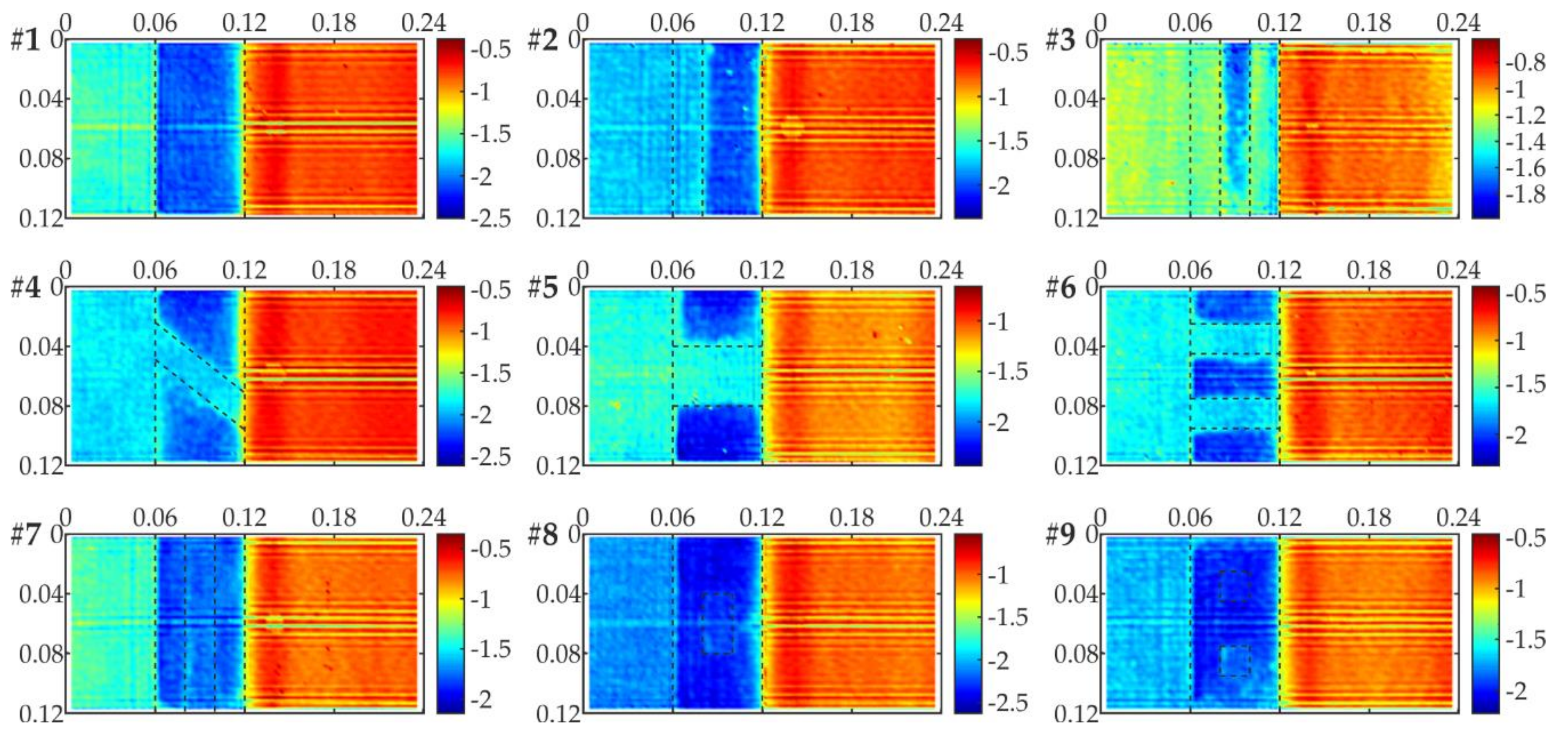
3.3.2. Influence of Defect Shape and Position
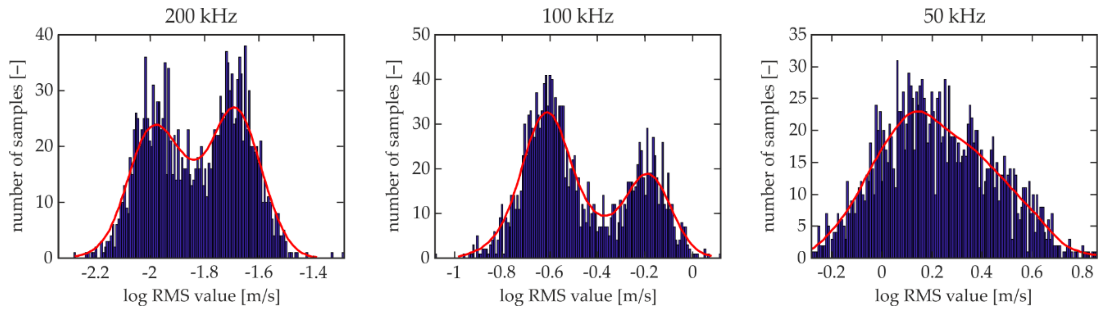
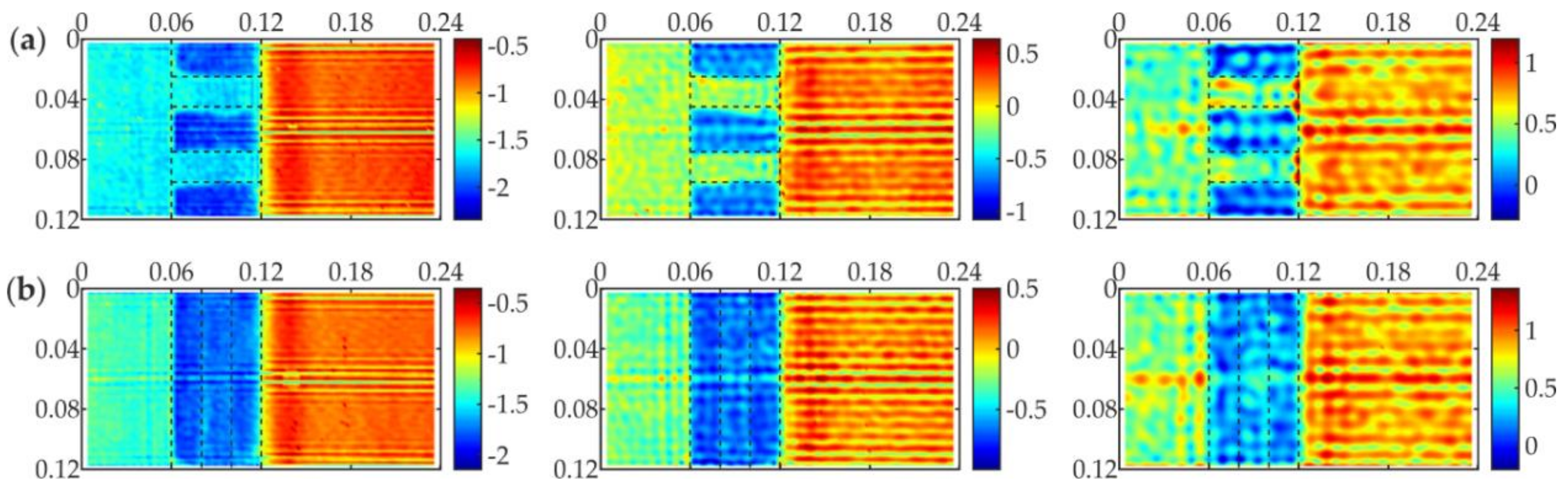
3.3.3. Influence of Excitation Frequency
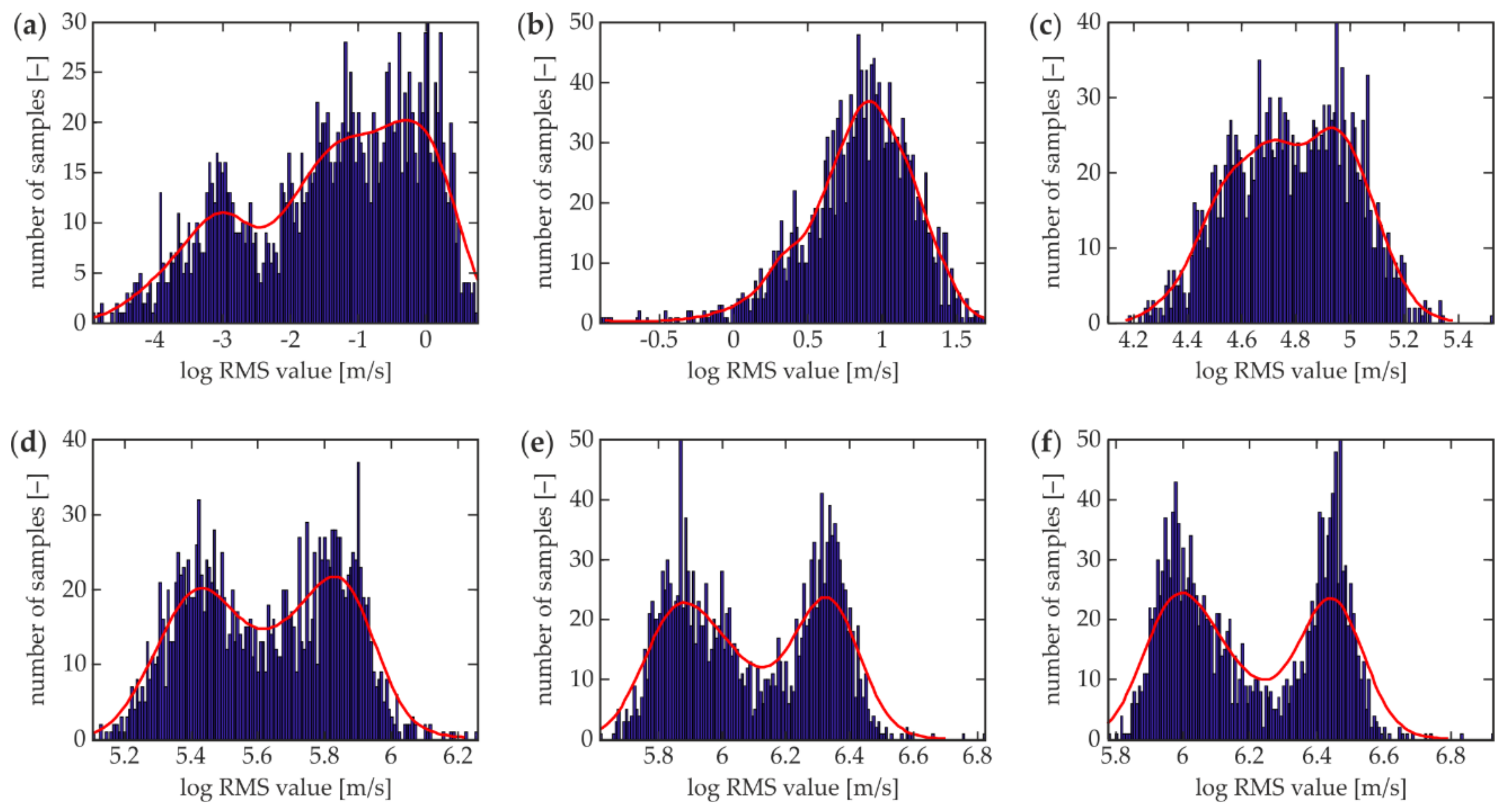
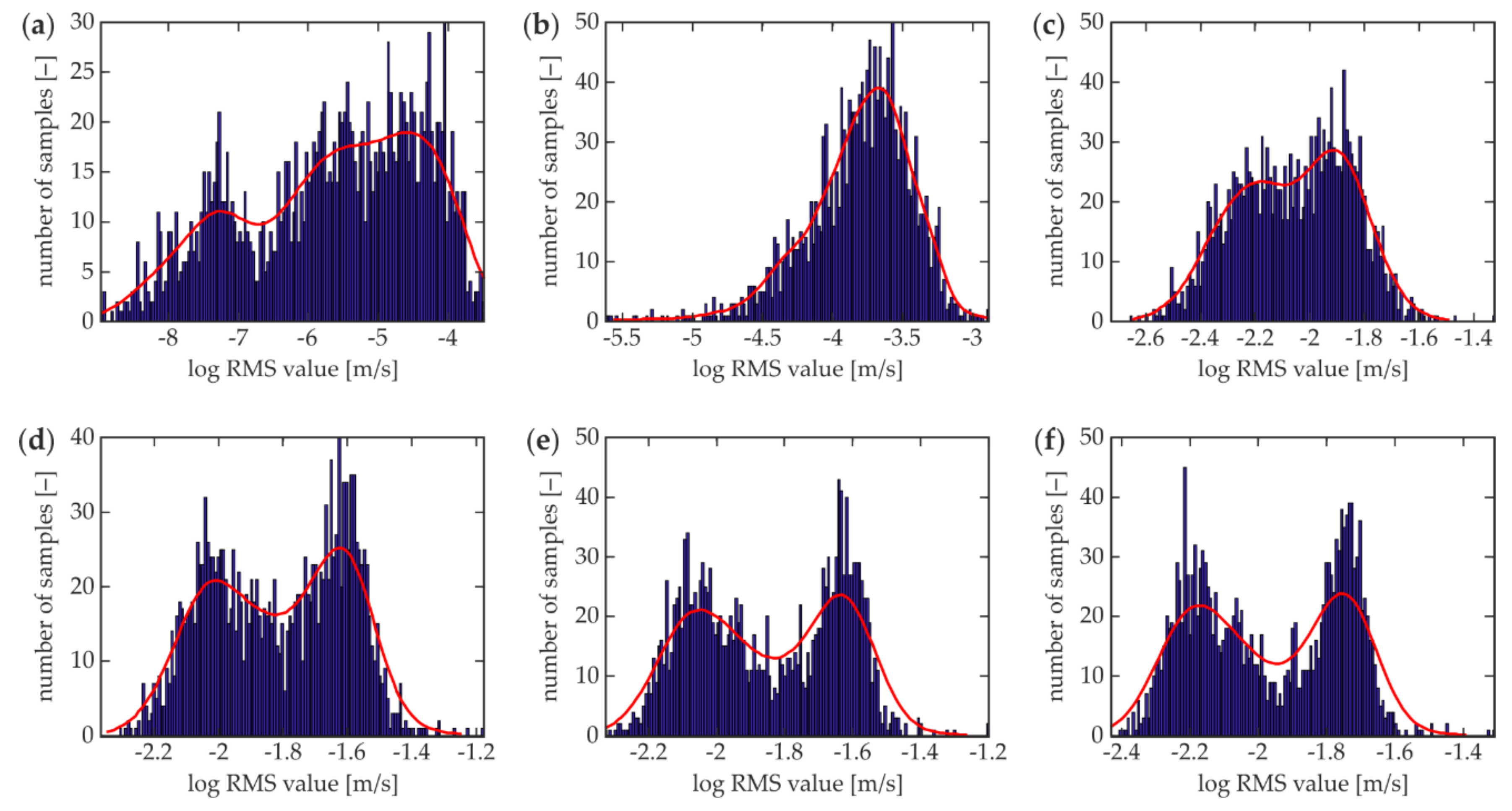
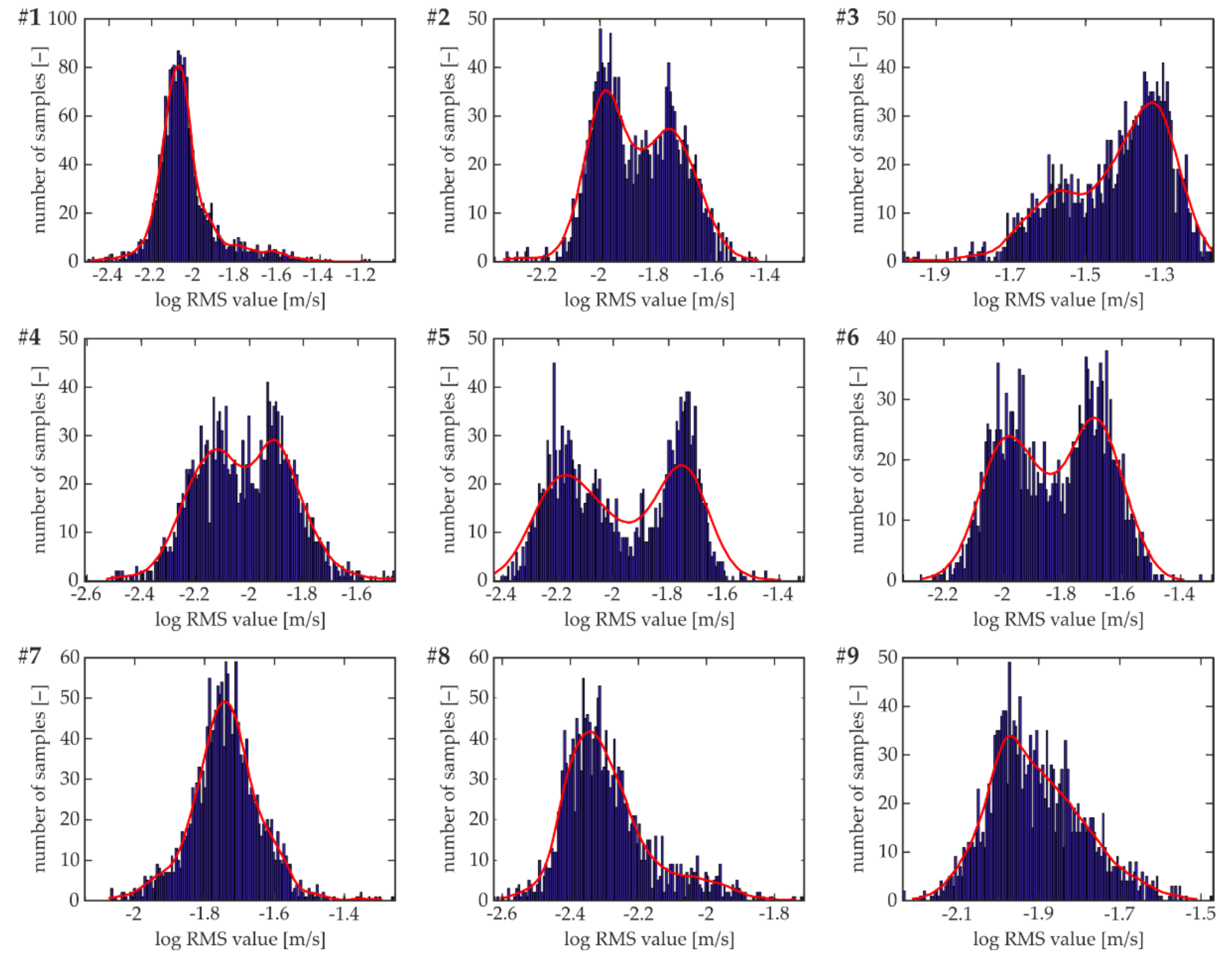
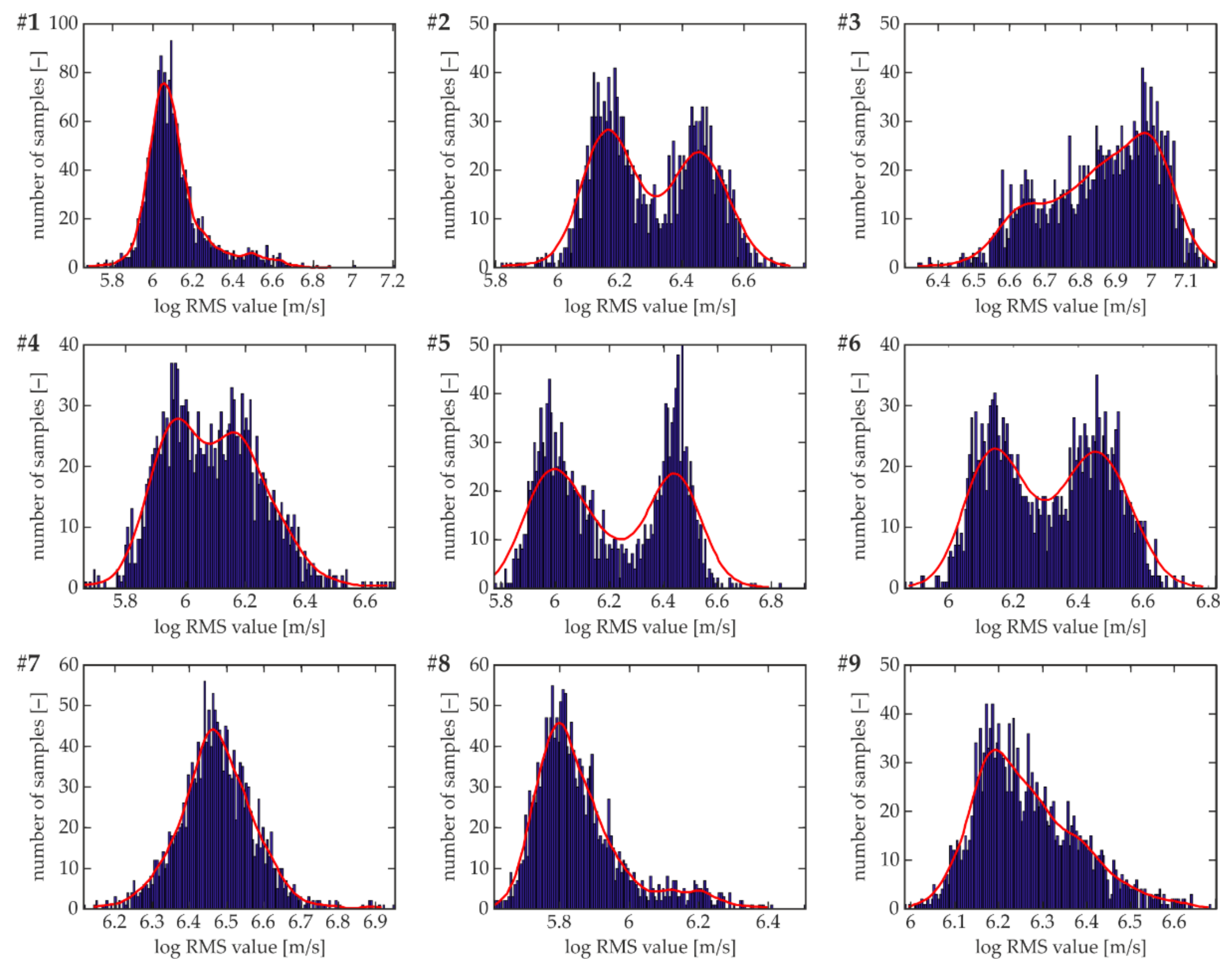
3.3.4. WRMS Histograms
4. Conclusions
- The analysis of maps that were obtained from the SLDV measurements provided the initial identification of defects with different efficiencies. The clearness of the SLDV maps varied depending on the shape and position of damage.
- The actual defect shape and location were determinable based on the appropriate damage imaging, where recorded out-of-plane vibrations were processed by means of the WMRS. The effectiveness of the applied method was strongly dependent on the calculation parameters (weighting factor and time window), excitation frequency, and a type of damage.
- The extension of the time window led to the increase in differences in the WRMS values between the damaged and undamaged areas of the adhesive joint. As a result, defects in the adhesive film could be identified more accurately.
- By comparing different variants of weighting factors, the constant one did not provide efficient results due to the high influence of the incident wave at the excitation point. This effect was reduced by the weighting factor, which was represented by the linear or square function that achieved comparable results. For specimens with internal defects, moderately greater effectiveness of the linear variant was observed.
- The shape and location of defects had a great impact on the effectiveness of their identification. Both the presence and the size of defects were possible to determine in all of the contested specimens based on the WRMS damage maps. The clearest results were obtained for stripe defects parallel or skewed to the primary direction of wave propagation. The disbonded areas in the shape of the strip perpendicular to the direction of wave propagation were also determinable, however, the identification was easier when such area was at the beginning or at the end of the lap. The most difficult to detect were the defects in the internal part of the adhesive film. The differentiation of effectiveness of the method for different types of defects resulted from the occurrence of different wave phenomena at the boundaries of defects. Stripe defects, skewed, or parallel to the direction of propagation triggered a diffraction of wave fronts that provided a significant disturbance in wave propagation and resulted in a higher intensification of signals. Defects in the shape of a perpendicular strip were related to wave reflection that did not disrupt the propagation as diffraction did. Finally, internal defects were the most difficult to identify because of the local characterization of occurring wave phenomena.
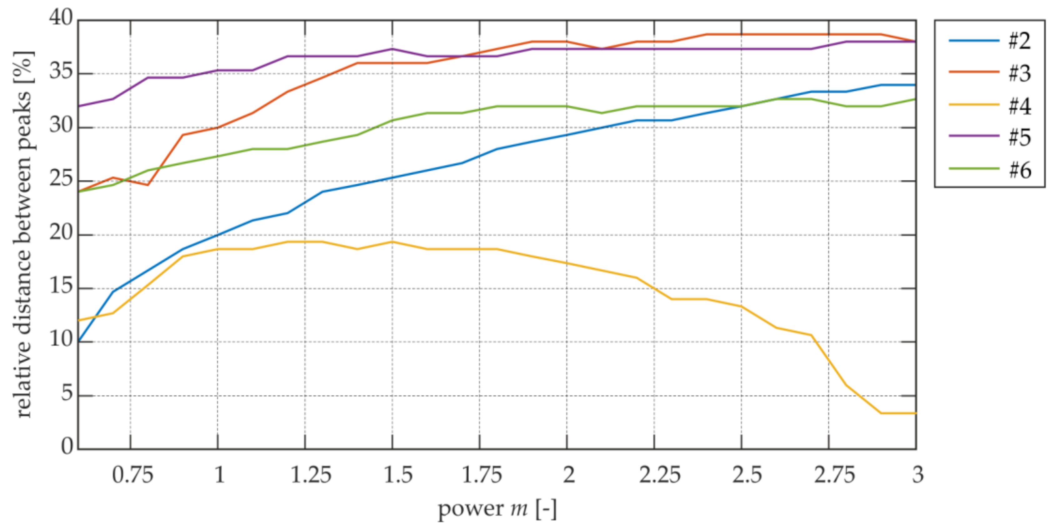
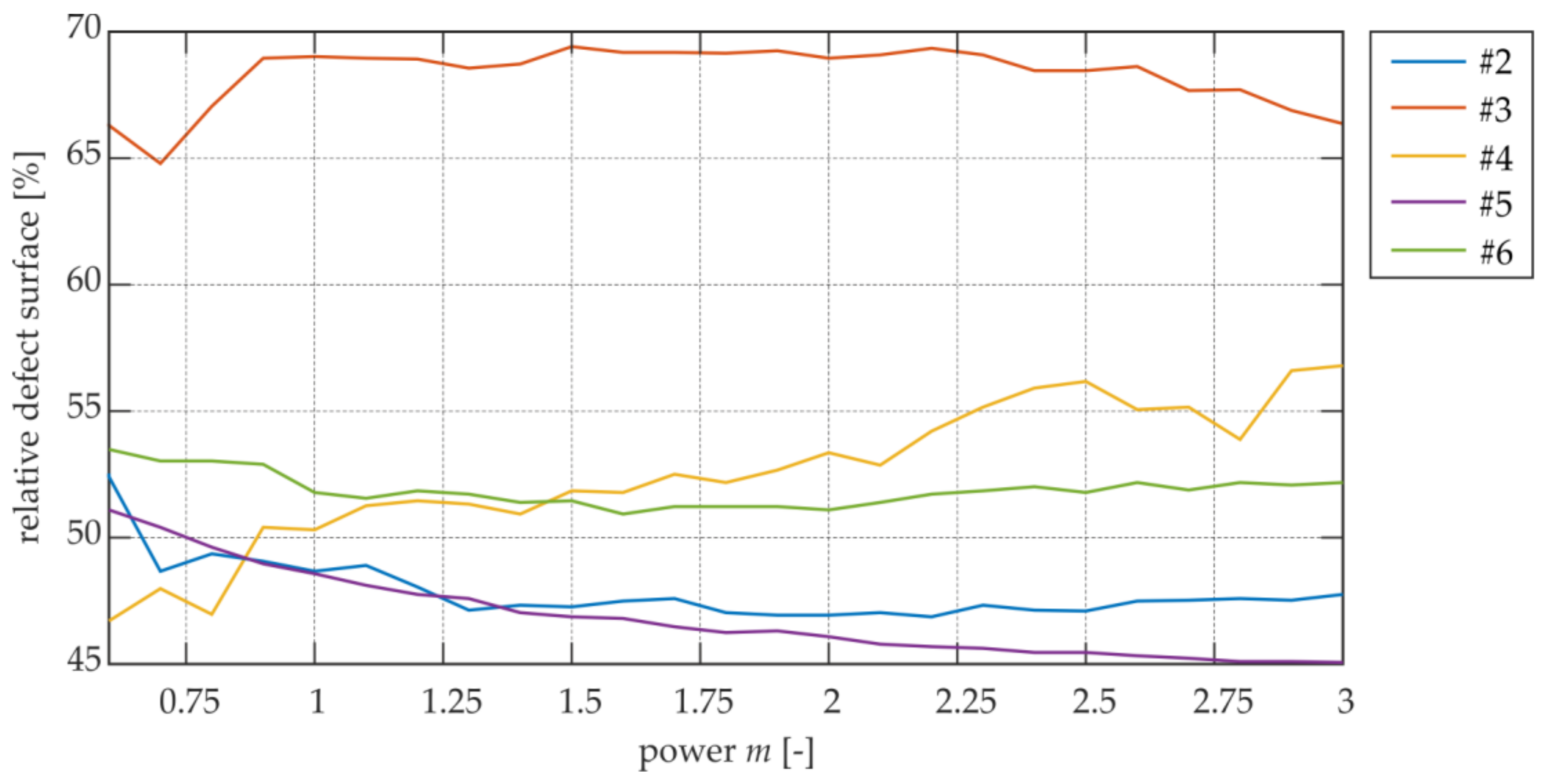
- The statistical analysis of the calculated WRMS values successfully supplemented the visual assessment of the damage images. The interpretation of the histograms helped to explain the effects that were observed on the WRMS maps. The use of the relative distance between peaks of bimodal distribution was proposed as the indicator for the optimal determination of WRMS parameters. Based on this indicator, it was proven that the largest value of the time window obtained damage maps with the highest clearness. Moreover, it was possible to determine the range of the optimal value of the weighting factor and to quantify the defect areas. The statistical analysis of the influence of the excitation frequency also enabled a comparison of the effectiveness of the three different frequencies. Two higher frequencies providing bimodal distribution were proven to be more effective than the lowest excitation frequency providing unimodal distribution.
Acknowledgments
Author Contributions
Conflicts of Interest
References
- Adams, R.D.; Wake, W.C. Structural Adhesive Joints in Engineering; Elsevier Applied Science Publishers: London, UK, 1986; ISBN 978-94-010-8977-7. [Google Scholar]
- Karachalios, E.F.; Adams, R.D.; Da Silva, L.F.M. Strength of single lap joints with artificial defects. Int. J. Adhes. Adhes. 2013, 45, 69–76. [Google Scholar] [CrossRef]
- Heidarpour, F.; Farahani, M.; Ghabezi, P. Experimental investigation of the effects of adhesive defects on the single lap joint strength. Int. J. Adhes. Adhes. 2018, 80, 128–132. [Google Scholar] [CrossRef]
- Jeenjitkaew, C.; Guild, F.J. The analysis of kissing bonds in adhesive joints. Int. J. Adhes. Adhes. 2017, 75, 101–107. [Google Scholar] [CrossRef]
- Adams, R.D.; Drinkwater, B.W. Nondestructive testing of adhesively-bonded joints. NDT E Int. 1997, 30, 93–98. [Google Scholar] [CrossRef]
- Korzeniowski, M.; Piwowarczyk, T.; Maev, R.G. Application of ultrasonic method for quality evaluation of adhesive layers. Arch. Civ. Mech. Eng. 2014, 14, 661–670. [Google Scholar] [CrossRef]
- Vijayakumar, R.L.; Bhat, M.R.; Murthy, C.R.L. Non destructive evaluation of adhesively bonded carbon fiber reinforced composite lap joints with varied bond quality. AIP Conf. Proc. 2012, 1430, 1276–1283. [Google Scholar] [CrossRef]
- Tighe, R.C.; Dulieu-Barton, J.M.; Quinn, S. Identification of kissing defects in adhesive bonds using infrared thermography. Int. J. Adhes. Adhes. 2016, 64, 168–178. [Google Scholar] [CrossRef]
- Vijaya Kumar, R.L.; Bhat, M.R.; Murthy, C.R.L. Evaluation of kissing bond in composite adhesive lap joints using digital image correlation: Preliminary studies. Int. J. Adhes. Adhes. 2013, 42, 60–68. [Google Scholar] [CrossRef]
- Vijaya kumar, R.L.; Bhat, M.R.; Murthy, C.R.L. Analysis of composite single lap joints using numerical and experimental approach. J. Adhes. Sci. Technol. 2014, 28, 893–914. [Google Scholar] [CrossRef]
- Roth, W.; Giurgiutiu, V. Structural health monitoring of an adhesive disbond through electromechanical impedance spectroscopy. Int. J. Adhes. Adhes. 2017, 73, 109–117. [Google Scholar] [CrossRef]
- Giurgiutiu, V. Structural Health Monitoring with Piezoelectric Wafer Active Sensors; Elsevier: Amsterdam, The Netherlands, 2008. [Google Scholar]
- Ostachowicz, W.; Kudela, P.; Krawczuk, M.; Zak, A. Guided Waves in Structures for SHM; Wiley: Hoboken, NJ, USA, 2012; ISBN 9781119965855. [Google Scholar]
- Rose, J.L. Ultrasonic Guided Waves in Solid Media; Cambridge University Press: New York, NY, USA, 2014; ISBN 9781107273610. [Google Scholar]
- Rokhlin, S. Lamb wave interaction with lap-shear adhesive joints: Theory and experiment. J. Acoust. Soc. Am. 1991, 89, 2758–2765. [Google Scholar] [CrossRef]
- Rose, J.L.; Rajana, K.M.; Hansch, M.K.T. Ultrasonic Guided Waves for NDE of Adhesively Bonded Structures. J. Adhes. 1995, 50, 71–82. [Google Scholar] [CrossRef]
- Lowe, M.J.S.; Challis, R.E.; Chan, C.W. The transmission of Lamb waves across adhesively bonded lap joints. J. Acoust. Soc. Am. 2000, 107, 1333–1345. [Google Scholar] [CrossRef] [PubMed]
- Di Scalea, F.L.; Bonomo, M.; Tuzzeo, D. Ultrasonic guided wave inspection of bonded lap joints: Noncontact method and photoelastic visualization. Res. Nondestruct. Eval. 2001, 13, 153–171. [Google Scholar] [CrossRef]
- Ren, B.; Lissenden, C.J. Ultrasonic guided wave inspection of adhesive bonds between composite laminates. Int. J. Adhes. Adhes. 2013, 45, 59–68. [Google Scholar] [CrossRef]
- Sherafat, M.H.; Quaegebeur, N.; Lessard, L.; Masson, P.; Hubert, P. Guided Wave Propagation through Composite Bonded Joints. In Proceedings of the EWSHM 7th European Workshop on Structural Health Monitoring, Nantes, France, 10 July 2014. [Google Scholar]
- Ren, B.; Lissenden, C.J. Modal content-based damage indicators for disbonds in adhesively bonded composite structures. Struct. Health Monit. Int. J. 2016, 15, 491–504. [Google Scholar] [CrossRef]
- Mori, N.; Biwa, S. Transmission of Lamb waves and resonance at an adhesive butt joint of plates. Ultrasonics 2016, 72, 80–88. [Google Scholar] [CrossRef] [PubMed]
- Gauthier, C.; El-Kettani, M.; Galy, J.; Predoi, M.; Leduc, D.; Izbicki, J.L. Lamb waves characterization of adhesion levels in aluminum/epoxy bi-layers with different cohesive and adhesive properties. Int. J. Adhes. Adhes. 2017, 74, 15–20. [Google Scholar] [CrossRef]
- Mallet, L.; Lee, B.C.; Staszewski, W.J.; Scarpa, F. Structural health monitoring using scanning laser vibrometry: II. Lamb waves for damage detection. Smart Mater. Struct. 2004, 13, 261–269. [Google Scholar] [CrossRef]
- Kudela, P.; Wandowski, T.; Malinowski, P.; Ostachowicz, W. Application of scanning laser Doppler vibrometry for delamination detection in composite structures. Opt. Lasers Eng. 2016, 99, 46–57. [Google Scholar] [CrossRef]
- Pieczonka, Ł.; Ambroziński, Ł.; Staszewski, W.J.; Barnoncel, D.; Pérès, P. Damage detection in composite panels based on mode-converted Lamb waves sensed using 3D laser scanning vibrometer. Opt. Lasers Eng. 2017, 99, 80–87. [Google Scholar] [CrossRef]
- Sunarsa, T.Y.; Aryan, P.; Jeon, I.; Park, B.; Liu, P.; Sohn, H. A reference-free and non-contact method for detecting and imaging damage in adhesive-bonded structures using air-coupled ultrasonic transducers. Materials (Basel) 2017, 10, 1402. [Google Scholar] [CrossRef]
- Esfandabadi, Y.K.; De Marchi, L.; Testoni, N.; Marzani, A.; Masetti, G. Full wavefield analysis and Damage imaging through compressive sensing in Lamb wave inspections. IEEE Trans. Ultrason. Ferroelectr. Freq. Control 2017, 65, 269–280. [Google Scholar] [CrossRef] [PubMed]
- Dziendzikowski, M.; Dragan, K.; Katunin, A. Localizing impact damage of composite structures with modified RAPID algorithm and non-circular PZT arrays. Arch. Civ. Mech. Eng. 2017, 17, 178–187. [Google Scholar] [CrossRef]
- Żak, A.; Radzieński, M.; Krawczuk, M.; Ostachowicz, W. Damage detection strategies based on propagation of guided elastic waves. Smart Mater. Struct. 2012, 21, 35024. [Google Scholar] [CrossRef]
- Radzieński, M.; Doliński, Ł.; Krawczuk, M.; Palacz, M. Damage localisation in a stiffened plate structure using a propagating wave. Mech. Syst. Signal Process. 2013, 39, 388–395. [Google Scholar] [CrossRef]
- Lee, C.; Park, S. Flaw Imaging Technique for Plate-Like Structures Using Scanning Laser Source Actuation. Shock Vib. 2014, 725030. [Google Scholar] [CrossRef]
- Jothi Saravanan, T.; Gopalakrishnan, N.; Prasad Rao, N. Damage detection in structural element through propagating waves using radially weighted and factored RMS. Meas. J. Int. Meas. Confed. 2015, 73, 520–538. [Google Scholar] [CrossRef]
- Geetha, G.K.; Roy Mahapatra, D.; Gopalakrishnan, S.; Hanagud, S. Laser Doppler imaging of delamination in a composite T-joint with remotely located ultrasonic actuators. Compos. Struct. 2016, 147, 197–210. [Google Scholar] [CrossRef]
- Marks, R.; Clarke, A.; Featherston, C.; Paget, C.; Pullin, R. Lamb Wave Interaction with Adhesively Bonded Stiffeners and Disbonds Using 3D Vibrometry. Appl. Sci. 2016, 6, 12. [Google Scholar] [CrossRef]
- Lee, C.; Zhang, A.; Yu, B.; Park, S. Comparison study between RMS and edge detection image processing algorithms for a pulsed laser UWPI (Ultrasonic wave propagation imaging)-based NDT technique. Sensors (Switzerland) 2017, 17, 1224. [Google Scholar] [CrossRef] [PubMed]
- Abràmoff, M.D.; Magalhães, P.J.; Ram, S.J. Image processing with imageJ. Biophotonics Int. 2004, 11, 36–41. [Google Scholar] [CrossRef]
- Alleyne, D.N.; Cawley, P. A 2-dimensional Fourier transform method for the quantitative measurement of Lamb modes. In Proceedings of the IEEE Ultrasonics Symposium, Honolulu, HI, USA, 4–7 December 1990; Volume 2, pp. 1143–1146. [Google Scholar] [CrossRef]
- Bocchini, P.; Asce, M.; Marzani, A.; Viola, E. Graphical User Interface for Guided Acoustic Waves. J. Comput. Civ. Eng. 2011, 25, 202–210. [Google Scholar] [CrossRef]
- Mazzotti, M.; Bartoli, I.; Marzani, A.; Viola, E. A coupled SAFE-2.5D BEM approach for the dispersion analysis of damped leaky guided waves in embedded waveguides of arbitrary cross-section. Ultrasonics 2013, 53, 1227–1241. [Google Scholar] [CrossRef] [PubMed]


| No. of Sample | Design Surface of Defect Area (cm2) | Determined Surface of Defect Area Including Kissing Defects (cm2) | Design Relative Defect Surface (%) | Determined Relative Defect Surface (%) |
|---|---|---|---|---|
| #1 | - | - | - | - |
| #2 | 24.00 | 24.00 | 33.33% | 33.33% |
| #3 | 48.00 | 49.11 | 66.67% | 68.21% |
| #4 | 15.00 | 17.64 | 20.83% | 24.50% |
| #5 | 24.00 | 26.03 | 33.33% | 36.16% |
| #6 | 24.00 | 26.33 | 33.33% | 36.57% |
| #7 | 24.00 | 29.55 | 33.33% | 41.05% |
| #8 | 8.00 | 9.09 | 11.11% | 12.63% |
| #9 | 8.00 | 13.34 | 11.11% | 18.53% |
| Time Window (ms) | Relative Peaks Distance (wr = r) (%) | Relative Peaks Distance (wr = r2) (%) |
|---|---|---|
| 0.03 | – | – |
| 0.05 | – | – |
| 0.50 | 18.67 | 12.67 |
| 1.00 | 30.67 | 33.33 |
| 2.00 | 34.67 | 34.67 |
| 3.00 | 35.33 | 37.33 |
© 2018 by the authors. Licensee MDPI, Basel, Switzerland. This article is an open access article distributed under the terms and conditions of the Creative Commons Attribution (CC BY) license (http://creativecommons.org/licenses/by/4.0/).
Share and Cite
Rucka, M.; Wojtczak, E.; Lachowicz, J. Damage Imaging in Lamb Wave-Based Inspection of Adhesive Joints. Appl. Sci. 2018, 8, 522. https://doi.org/10.3390/app8040522
Rucka M, Wojtczak E, Lachowicz J. Damage Imaging in Lamb Wave-Based Inspection of Adhesive Joints. Applied Sciences. 2018; 8(4):522. https://doi.org/10.3390/app8040522
Chicago/Turabian StyleRucka, Magdalena, Erwin Wojtczak, and Jacek Lachowicz. 2018. "Damage Imaging in Lamb Wave-Based Inspection of Adhesive Joints" Applied Sciences 8, no. 4: 522. https://doi.org/10.3390/app8040522
APA StyleRucka, M., Wojtczak, E., & Lachowicz, J. (2018). Damage Imaging in Lamb Wave-Based Inspection of Adhesive Joints. Applied Sciences, 8(4), 522. https://doi.org/10.3390/app8040522