A Semantic Segmentation Algorithm Using FCN with Combination of BSLIC


Abstract
:1. Introduction
2. Related Work
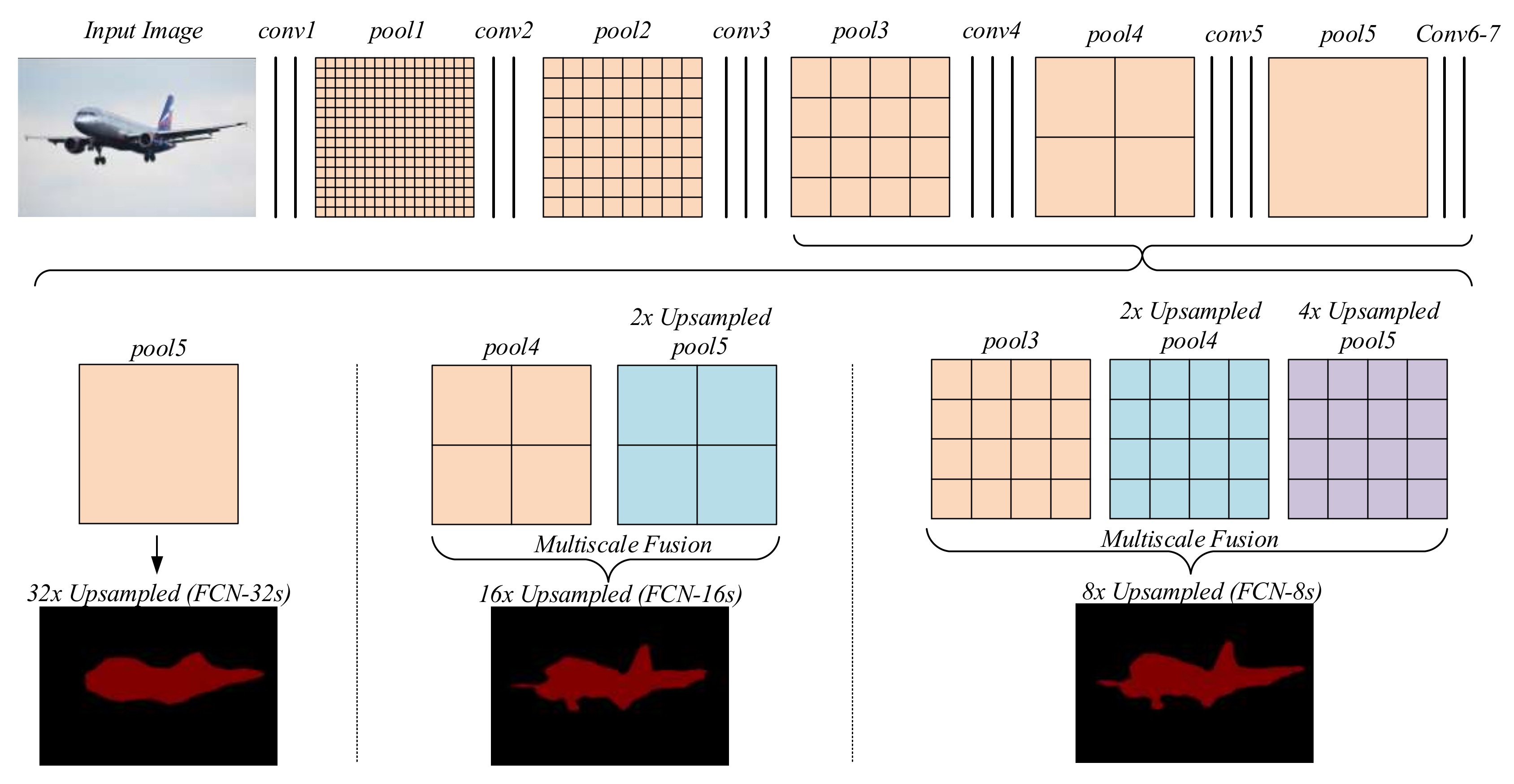
2.1. FCN
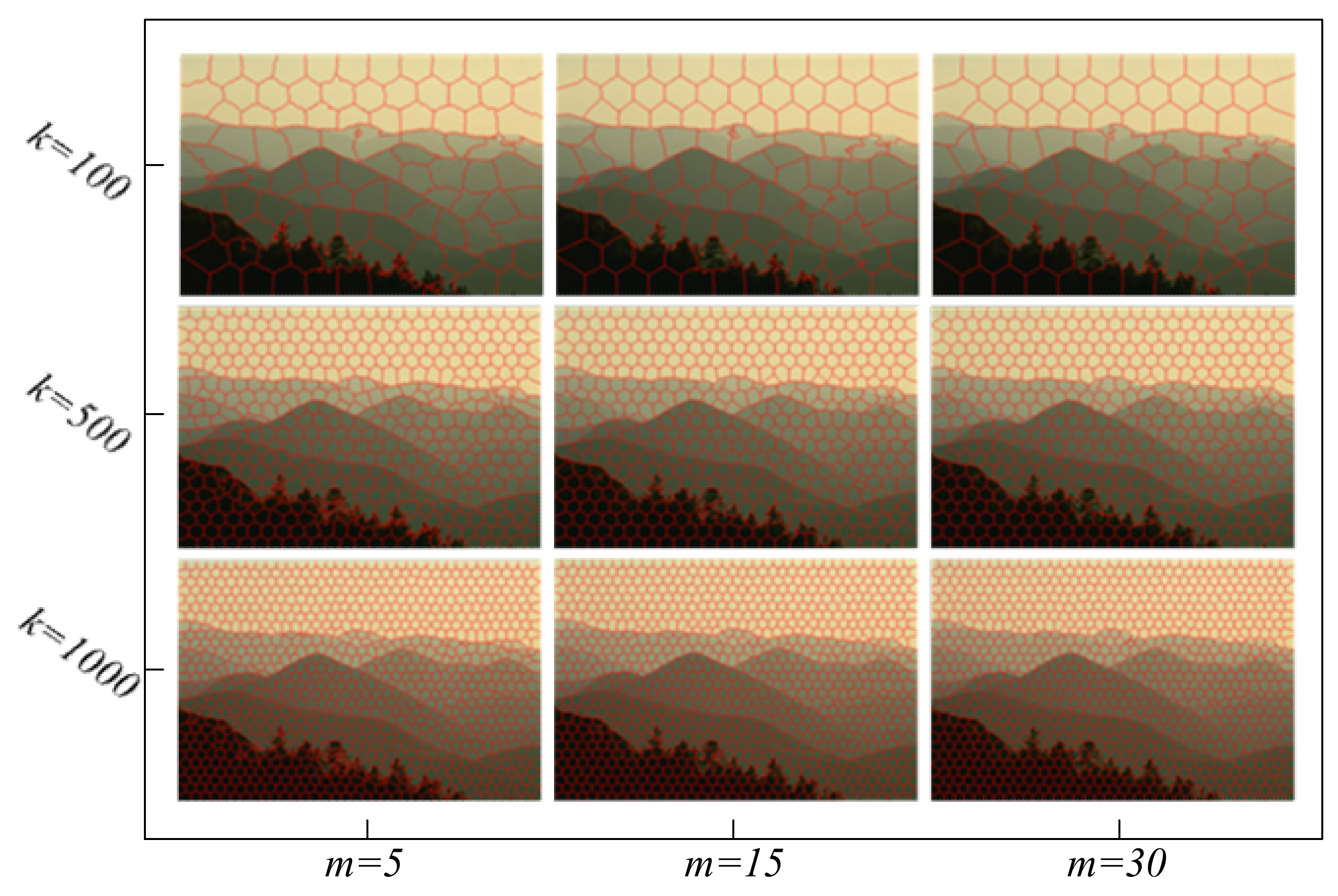
2.2. BSLIC
3. Proposed Algorithm
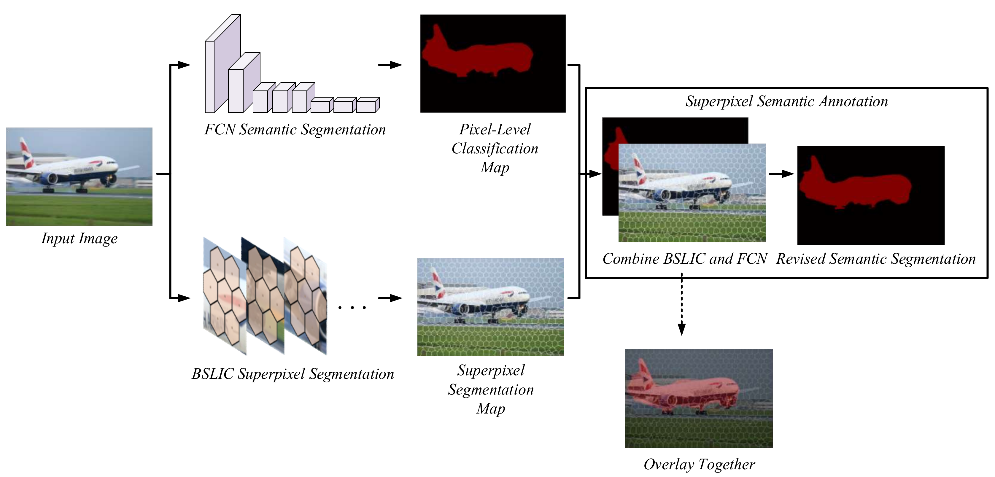
3.1. Overall Framwork
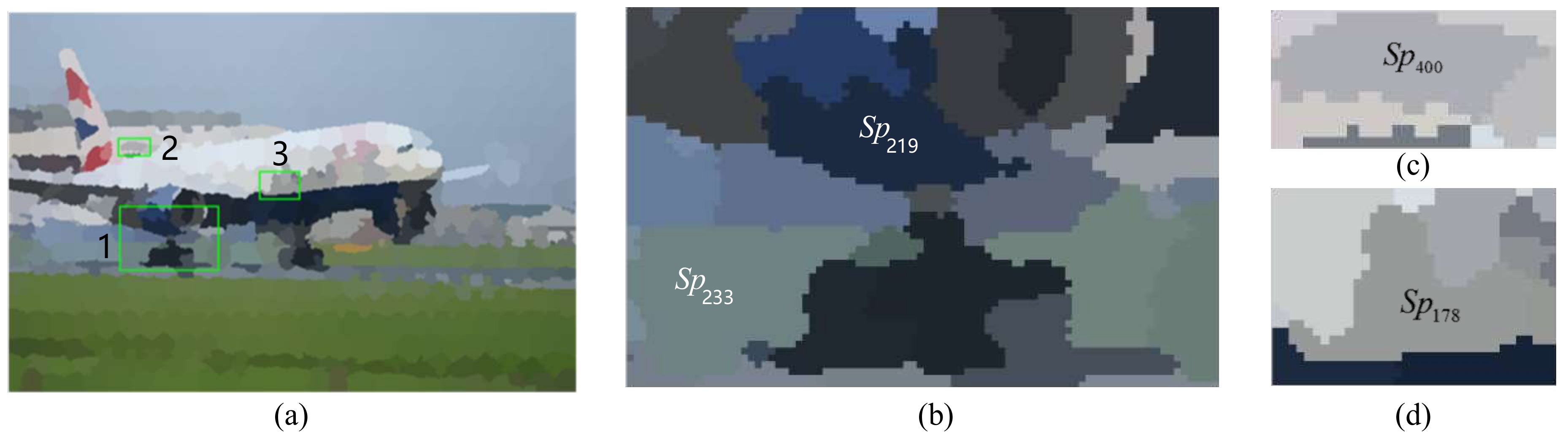
3.2. Superpixel Semantic Annotation
| Algorithm 1. Superpixel semantic annotation | ||
| 1. | Acquire a FCN pixel-level classification map. | |
| 2. | Acquire a BSLIC superpixel segmentation map. The parameters are shown as follows: the collection of superpixel , the number of semantic categories in superpixel is A, the proportion of pixels of the semantic category t() , all pixels in the superpixel is . | |
| 3. | Generate superpixel semantic annotation using the four criteria | |
| Loop: For | ||
| Criterion 1 | If there is no image edge in superpixel and then Label the superpixel with FCN semantic result End | |
| Criterion 2 | If there is no image edge in superpixel and then Use t of the largest to label the superpixel End | |
| Criterion 3 | If there is image edge in superpixel and then Label the superpixel with FCN semantic result End | |
| Criterion 4 | If there is image edge in superpixel and then If > 80% in superpixel then
End | |
| 4. | Output the superpixel semantic annotation result. | |
4. Experimental Results
4.1. Training and Testing of FCN Model
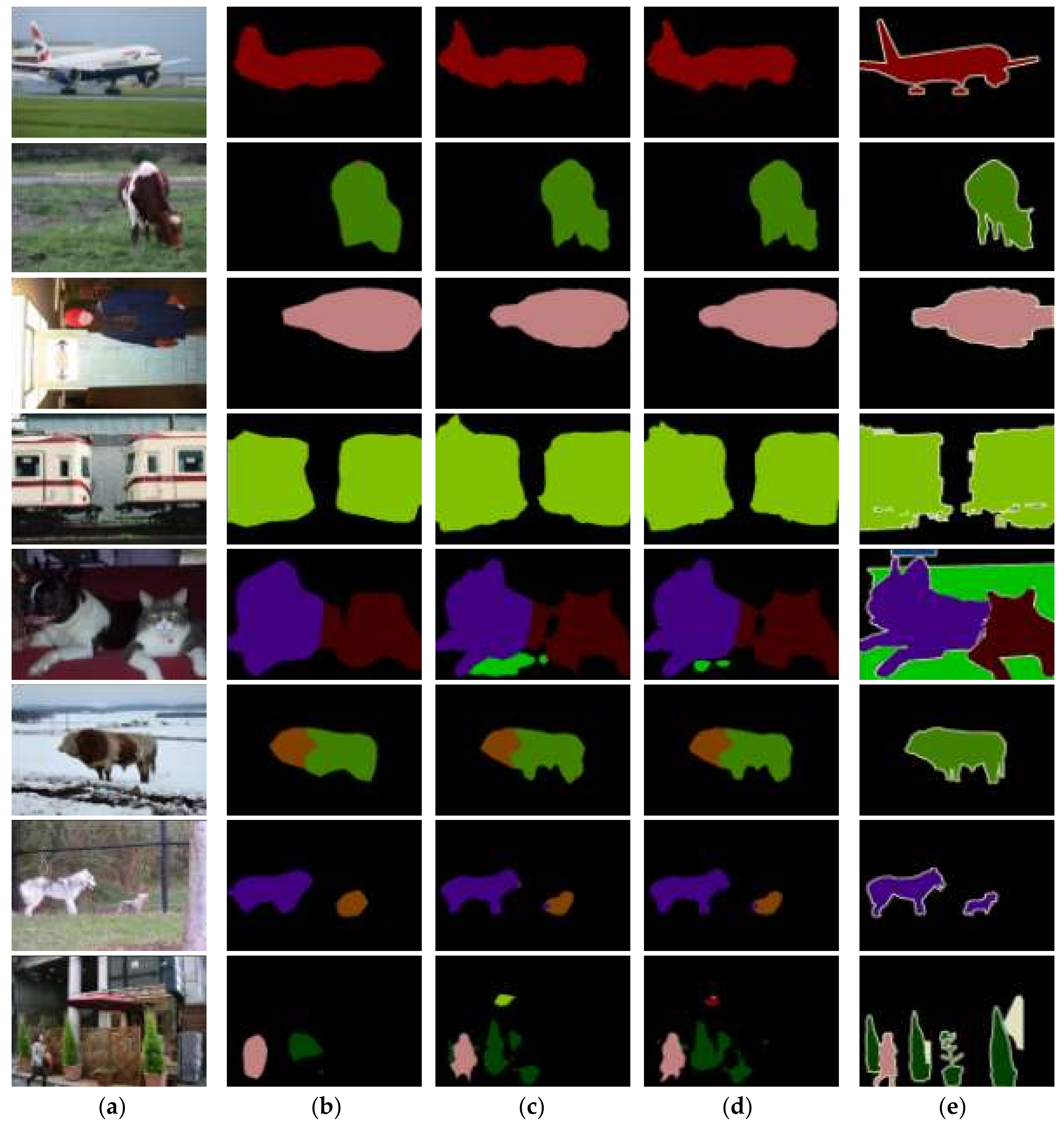
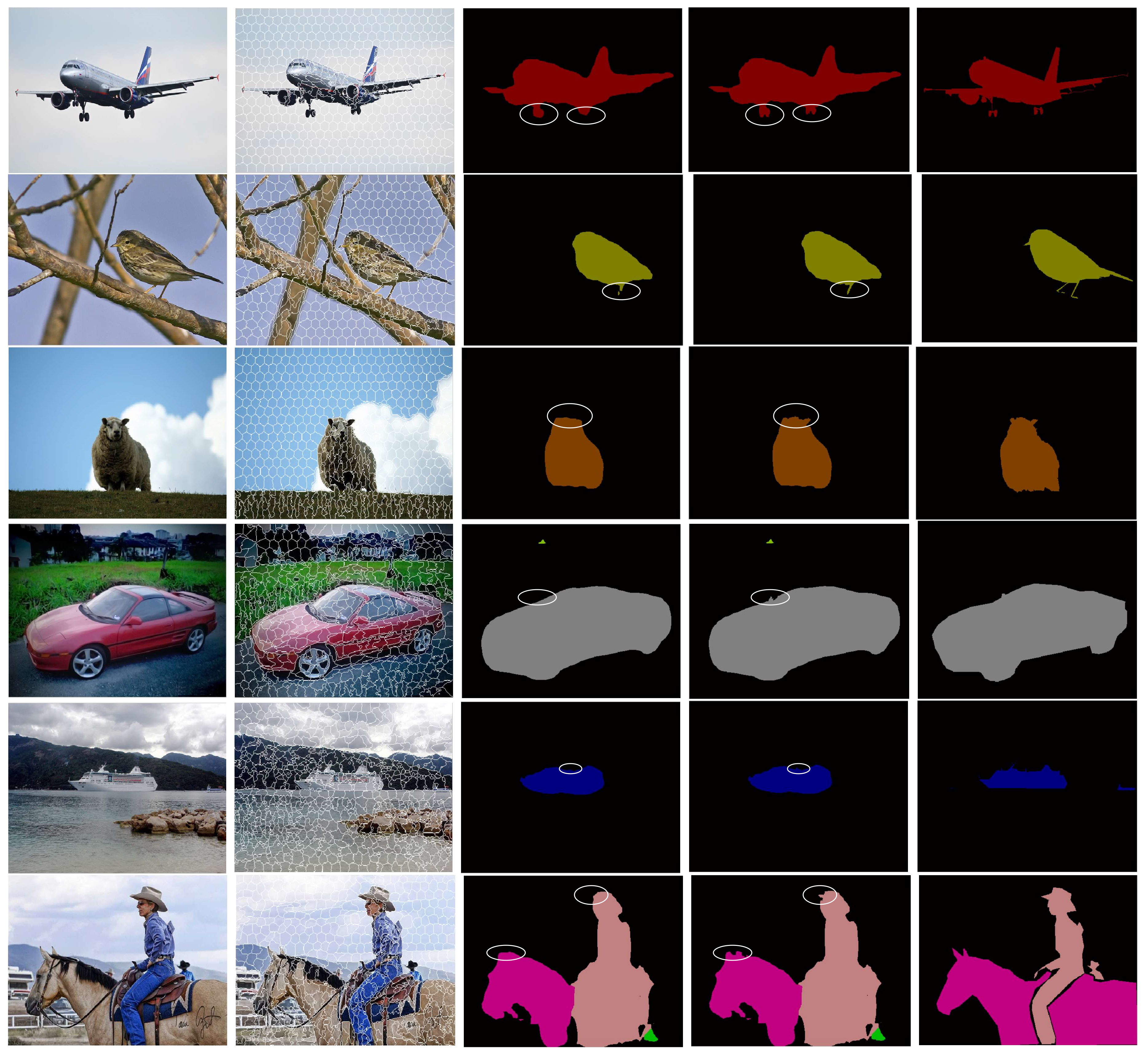
4.2. Qualitative Comparison
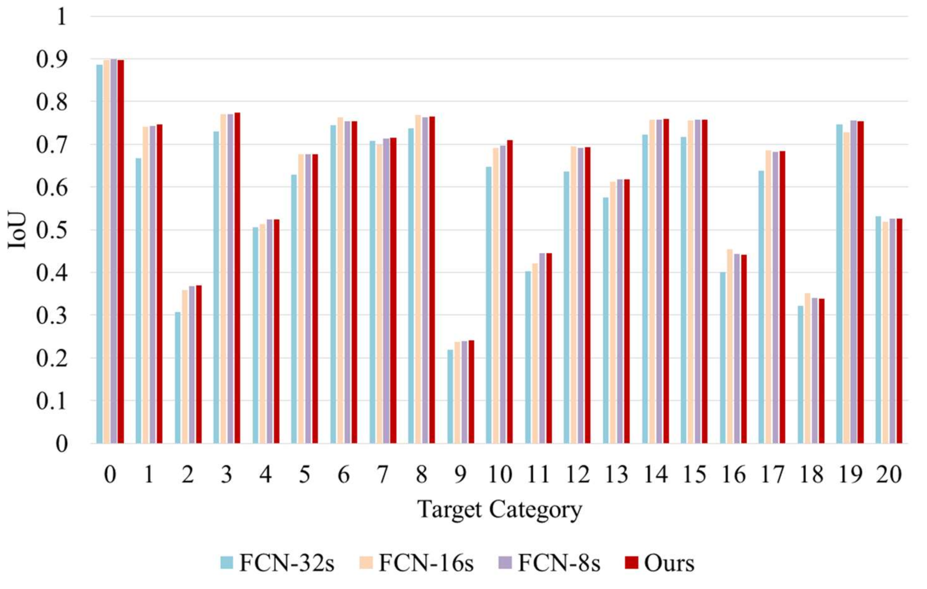
4.3. Quantitative Comparison
5. Conclusions
Author Contributions
Conflicts of Interest
References
- Feldman, J.A.; Yakimovsky, Y. Decision theory and artificial intelligence: I. A semantics-based region analyzer. Artif. Intell. 1974, 5, 349–371. [Google Scholar]
- Yang, L.; Meer, P.; Foran, D.J. Multiple class segmentation using a unified framework over mean-shift patches. In Proceedings of the 2007 IEEE Conference on Computer Vision and Pattern Recognition, CVPR’07, Minneapolis, MN, USA, 17–22 June 2007; pp. 1–8. [Google Scholar]
- Arbeláez, P.; Pont-Tuset, J.; Barron, J.T.; Marques, F.; Malik, J. Multiscale combinatorial grouping. In Proceedings of the IEEE Conference on Computer Vision and Pattern Recognition, Columbus, OH, USA, 23–28 June 2014; pp. 328–335. [Google Scholar]
- Long, J.; Shelhamer, E.; Darrell, T. Fully convolutional networks for semantic segmentation. In Proceedings of the IEEE Conference on Computer Vision and Pattern Recognition, Boston, MA, USA, 7–12 June 2015; pp. 3431–3440. [Google Scholar]
- Chen, L.C.; Papandreou, G.; Kokkinos, I.; Murphy, K.; Yuille, A.L. Semantic image segmentation with deep convolutional nets and fully connected crfs. Comput. Sci. 2014, 357–361. [Google Scholar]
- Noh, H.; Hong, S.; Han, B. Learning deconvolution network for semantic segmentation. In Proceedings of the IEEE International Conference on Computer Vision, Los Alamitos, CA, USA, 7–13 December 2015; pp. 1520–1528. [Google Scholar]
- Mostajabi, M.; Yadollahpour, P.; Shakhnarovich, G. Feedforward semantic segmentation with zoom-out features. In Proceedings of the IEEE Conference on Computer Vision and Pattern Recognition, Boston, MA, USA, 7–12 June 2015; pp. 3376–3385. [Google Scholar]
- Chen, L.-C.; Yang, Y.; Wang, J.; Xu, W.; Yuille, A.L. Attention to scale: Scale-aware semantic image segmentation. In Proceedings of the IEEE Conference on Computer Vision and Pattern Recognition, Seattle, WA, USA, 27–30 June 2016; pp. 3640–3649. [Google Scholar]
- Chen, L.-C.; Papandreou, G.; Kokkinos, I.; Murphy, K.; Yuille, A.L. Deeplab: Semantic image segmentation with deep convolutional nets, atrous convolution, and fully connected crfs. arXiv, 2016; arXiv:1606.00915. [Google Scholar]
- Taskar, B.; Abbeel, P.; Koller, D. Discriminative probabilistic models for relational data. In Proceedings of the Eighteenth Conference on Uncertainty in Artificial Intelligence, Edmonton, AB, Canada, 1–4 August 2002; pp. 485–492. [Google Scholar]
- Lafferty, J.D.; Mccallum, A.; Pereira, F.C.N. Conditional random fields: Probabilistic models for segmenting and labeling sequence data. In Proceedings of the Eighteenth International Conference on Machine Learning, Williamstown, MA, USA, 28 June–1 July 2001; pp. 282–289. [Google Scholar]
- Russell, B.C.; Torralba, A.; Murphy, K.P.; Freeman, W.T. Labelme: A database and web-based tool for image annotation. Int. J. Comput. Vis. 2008, 77, 157–173. [Google Scholar] [CrossRef]
- Carreira, J.; Li, F.; Sminchisescu, C. Object recognition by sequential figure-ground ranking. Int. J. Comput. Vis. 2012, 98, 243–262. [Google Scholar] [CrossRef]
- Uijlings, J.R.; Van De Sande, K.E.; Gevers, T.; Smeulders, A.W. Selective search for object recognition. Int. J. Comput. Vis. 2013, 104, 154–171. [Google Scholar] [CrossRef]
- Girshick, R. Fast R-CNN. In Proceedings of the IEEE International Conference on Computer Vision, Santiago, Chile, 7–13 December 2015; pp. 1440–1448. [Google Scholar]
- He, K.; Zhang, X.; Ren, S.; Sun, J. Spatial pyramid pooling in deep convolutional networks for visual recognition. IEEE Trans. Pattern Anal. Mach. Intell. 2015, 37, 1904–1916. [Google Scholar] [CrossRef] [PubMed]
- Ren, S.; He, K.; Girshick, R.; Sun, J. Faster R-CNN: Towards real-time object detection with region proposal networks. Adv. Neural Inf. Process. Syst. 2015, 39, 91–99. [Google Scholar] [CrossRef] [PubMed]
- Carreira, J.; Sminchisescu, C. Cpmc: Automatic object segmentation using constrained parametric min-cuts. IEEE Trans. Pattern Anal. Mach. Intell. 2012, 34, 1312–1328. [Google Scholar] [CrossRef] [PubMed]
- Liu, S.; Qi, X.; Shi, J.; Zhang, H.; Jia, J. Multi-scale patch aggregation (mpa) for simultaneous detection and segmentation. In Proceedings of the IEEE Conference on Computer Vision and Pattern Recognition, Seattle, WA, USA, 27–30 June 2016; pp. 3141–3149. [Google Scholar]
- Krizhevsky, A.; Sutskever, I.; Hinton, G.E. Imagenet classification with deep convolutional neural networks. Adv. Neural Inf. Process. Syst. 2012, 1097–1105. [Google Scholar] [CrossRef]
- Simonyan, K.; Zisserman, A. Very deep convolutional networks for large-scale image recognition. arXiv, 2014; arXiv:1409.1556. [Google Scholar]
- Szegedy, C.; Liu, W.; Jia, Y.; Sermanet, P.; Reed, S.; Anguelov, D.; Erhan, D.; Vanhoucke, V.; Rabinovich, A. Going deeper with convolutions. arXiv, 2015; arXiv:1409.4842. [Google Scholar]
- Ren, X.; Malik, J. Learning a classification model for segmentation. In Proceedings of the Ninth IEEE International Conference on Computer Vision, Nice, France, 13–16 October 2003; p. 10. [Google Scholar]
- Levinshtein, A.; Stere, A.; Kutulakos, K.N.; Fleet, D.J.; Dickinson, S.J.; Siddiqi, K. Turbopixels: Fast superpixels using geometric flows. IEEE Trans. Pattern Anal. Mach. Intell. 2009, 31, 2290–2297. [Google Scholar] [CrossRef] [PubMed]
- Zhang, Y.; Hartley, R.; Mashford, J.; Burn, S. Superpixels via pseudo-boolean optimization. In Proceedings of the 2011 IEEE International Conference on Computer Vision (ICCV), Barcelona, Spain, 6–13 November 2011; pp. 1387–1394. [Google Scholar]
- Van den Bergh, M.; Boix, X.; Roig, G.; de Capitani, B.; Van Gool, L. Seeds: Superpixels extracted via energy-driven sampling. In Proceedings of the European Conference on Computer Vision, Florence, Italy, 7–13 October 2012; pp. 13–26. [Google Scholar]
- Achanta, R.; Shaji, A.; Smith, K.; Lucchi, A.; Fua, P.; Süsstrunk, S. Slic superpixels compared to state-of-the-art superpixel methods. IEEE Trans. Pattern Anal. Mach. Intell. 2012, 34, 2274–2282. [Google Scholar] [CrossRef] [PubMed]
- Wang, H.; Peng, X.; Xiao, X.; Liu, Y. Bslic: Slic superpixels based on boundary term. Symmetry 2017, 9, 31. [Google Scholar] [CrossRef]
- Wang, H.; Xiao, X.; Peng, X.; Liu, Y.; Zhao, W. Improved image denoising algorithm based on superpixel clustering and sparse representation. Appl. Sci. 2017, 7, 436. [Google Scholar] [CrossRef]
- Hariharan, B.; Arbeláez, P.; Bourdev, L.; Maji, S.; Malik, J. Semantic contours from inverse detectors. In Proceedings of the 2011 IEEE International Conference on Computer Vision (ICCV), Barcelona, Spain, 6–13 November 2011; pp. 991–998. [Google Scholar]
- Garcia-Garcia, A.; Orts-Escolano, S.; Oprea, S.; Villena-Martinez, V.; Garcia-Rodriguez, J. A review on deep learning techniques applied to semantic segmentation. arXiv, 2017; arXiv:1704.06857. [Google Scholar]
- Badrinarayanan, V.; Kendall, A.; Cipolla, R. Segnet: A deep convolutional encoder-decoder architecture for scene segmentation. IEEE Trans. Pattern Anal. Mach. Intell. 2017, 39, 2481–2495. [Google Scholar] [CrossRef] [PubMed]
- Nekrasov, V.; Ju, J.; Choi, J. Global deconvolutional networks for semantic segmentation. arXiv, 2016; arXiv:1602.03930. [Google Scholar]


| Method | Average Time (ms/image) |
|---|---|
| FCN-32s | 293.050 |
| FCN-16s | 297.358 |
| FCN-8s | 302.796 |
| Ours | 310.218 |
| Category | SegNet | UNIST_GDN_FCN | Ours |
|---|---|---|---|
| 0 | 90.3 * | 89.8 | 89.7 |
| 1 | 73.6 | 74.5 | 74.7 * |
| 2 | 37.6 * | 31.9 | 36.9 |
| 3 | 62.0 | 66.7 | 77.4 * |
| 4 | 46.8 | 49.7 | 52.4 * |
| 5 | 58.6 | 60.5 | 67.7 * |
| 6 | 79.1 * | 76.9 | 75.5 |
| 7 | 70.1 | 75.9 * | 71.5 |
| 8 | 65.4 | 76.0 | 76.5 * |
| 9 | 23.6 | 22.9 | 24.1 * |
| 10 | 60.4 | 57.6 | 71.0 * |
| 11 | 45.6 | 54.5 * | 44.6 |
| 12 | 61.8 | 73.0 * | 69.3 |
| 13 | 63.5 * | 59.4 | 61.8 |
| 14 | 75.3 | 75.0 | 76.0 * |
| 15 | 74.9 | 73.7 | 75.8 * |
| 16 | 42.6 | 51.0 * | 44.1 |
| 17 | 63.7 | 67.5 | 68.5 * |
| 18 | 42.5 | 43.3 * | 33.9 |
| 19 | 67.8 | 70.0 | 75.4 * |
| 20 | 52.7 | 56.4 * | 52.6 |
| Category | FCN-32s | FCN-16s | FCN-8s | Ours |
|---|---|---|---|---|
| 0 | 88.611 | 89.704 | 89.961 * | 89.721 |
| 1 | 66.803 | 74.143 | 74.346 | 74.676 * |
| 2 | 30.772 | 35.861 | 36.759 | 36.899 * |
| 3 | 72.928 | 77.133 | 77.016 | 77.426 * |
| 4 | 50.662 | 51.285 | 52.407 * | 52.357 |
| 5 | 62.929 | 67.623 | 67.688 | 67.718 * |
| 6 | 74.483 | 76.308 * | 75.414 | 75.484 |
| 7 | 70.754 | 69.941 | 71.397 | 71.527 * |
| 8 | 73.813 | 76.879 * | 76.312 | 76.452 |
| 9 | 21.913 | 23.666 | 23.923 | 24.133 * |
| 10 | 64.795 | 69.183 | 69.738 | 71.048 * |
| 11 | 40.358 | 42.070 | 44.482 | 44.562 * |
| 12 | 63.655 | 69.423 * | 69.171 | 69.331 |
| 13 | 57.512 | 61.184 | 61.781 | 61.801 * |
| 14 | 72.333 | 75.706 | 75.693 | 75.973 * |
| 15 | 71.729 | 75.618 | 75.740 | 75.830 * |
| 16 | 40.177 | 45.430 * | 44.259 | 44.079 |
| 17 | 63.780 | 68.546 * | 68.189 | 68.469 |
| 18 | 32.200 | 35.057 * | 34.077 | 33.877 |
| 19 | 74.669 | 72.746 | 75.508 * | 75.378 |
| 20 | 53.204 * | 51.937 | 52.681 | 52.561 |
| Compare 1 | Compare 2 | Compare 3 | ||||
|---|---|---|---|---|---|---|
| Method | Ours | FCN-32s | Ours | FCN-16s | Ours | FCN-8s |
| Advantage Category | 20 | 1 | 15 | 6 | 16 | 5 |
| Increased Ratio | 95.24% (20/21) | 71.43% (15/21) | 76.19% (16/21) | |||
| Metric | mIoU | PA |
|---|---|---|
| FCN-32s | 59.4 | 73.27 |
| FCN-16s | 62.3 | 75.73 |
| FCN-8s | 62.6 | 75.85 |
| Ours | 62.8 * | 77.14 * |
| SegNet | 59.9 | - |
| UNIST_GDN_FCN | 62.2 | - |
© 2018 by the authors. Licensee MDPI, Basel, Switzerland. This article is an open access article distributed under the terms and conditions of the Creative Commons Attribution (CC BY) license (http://creativecommons.org/licenses/by/4.0/).
Share and Cite
Zhao, W.; Zhang, H.; Yan, Y.; Fu, Y.; Wang, H. A Semantic Segmentation Algorithm Using FCN with Combination of BSLIC. Appl. Sci. 2018, 8, 500. https://doi.org/10.3390/app8040500
Zhao W, Zhang H, Yan Y, Fu Y, Wang H. A Semantic Segmentation Algorithm Using FCN with Combination of BSLIC. Applied Sciences. 2018; 8(4):500. https://doi.org/10.3390/app8040500
Chicago/Turabian StyleZhao, Wei, Haodi Zhang, Yujin Yan, Yi Fu, and Hai Wang. 2018. "A Semantic Segmentation Algorithm Using FCN with Combination of BSLIC" Applied Sciences 8, no. 4: 500. https://doi.org/10.3390/app8040500
APA StyleZhao, W., Zhang, H., Yan, Y., Fu, Y., & Wang, H. (2018). A Semantic Segmentation Algorithm Using FCN with Combination of BSLIC. Applied Sciences, 8(4), 500. https://doi.org/10.3390/app8040500