Polyphonic Piano Transcription with a Note-Based Music Language Model

Abstract

This paper proposes a note-based music language model (MLM) for improving note-level polyphonic piano transcription. The MLM is based on the recurrent structure, which could model the temporal correlations between notes in music sequences. To combine the outputs of the note-based MLM and acoustic model directly, an integrated architecture is adopted in this paper. We also propose an inference algorithm, in which the note-based MLM is used to predict notes at the blank onsets in the thresholding transcription results. The experimental results show that the proposed inference algorithm improves the performance of note-level transcription. We also observe that the combination of the restricted Boltzmann machine (RBM) and recurrent structure outperforms a single recurrent neural network (RNN) or long short-term memory network (LSTM) in modeling the high-dimensional note sequences. Among all the MLMs, LSTM-RBM helps the system yield the best results on all evaluation metrics regardless of the performance of acoustic models.

1. Introduction

Automatic music transcription (AMT) is a process that aims to convert a music signal into a symbolic notation. It is a fundamental problem of music information retrieval and has many applications in related fields, such as music education and composition. AMT has been researched for decades [1], and the transcription of polyphonic music remains to be unsolved [2]. The concurrent notes overlap in the time domain and interact in the frequency domain so that the polyphonic signal is complex. Piano is a typical multi-pitch instrument and has a wide playing range of 88 pitches. As a challenging task in polyphonic AMT, piano transcription has been studied extensively [3].

The note is the basic unit of music, as well as of notations. The main purpose of AMT is to figure out which notes are played and when they appear in the music, corresponding to a note-level transcription. The approaches to note extraction can be divided into frame-based methods and note-based methods. The frame-based approaches estimate pitches in each time frame and form frame-level results. The most straightforward solution is to analyze the time-frequency representation of audio and estimate pitches by detecting peaks in the spectrum [4]. Short time Fourier transform (STFT) [5,6] and constant Q transform (CQT) [7] are two widely-used time-frequency analysis methods. Spectrogram factorization techniques are also very popular in AMT, such as non-negative matrix factorization (NMF) [8] and probabilistic latent component analysis (PLCA) [9,10]. The activations of factorization indicate which pitch is active at the given time frame. Recently, many deep neural networks have been used to identify pitches and provided satisfying performance [11,12,13]. However, the frame-level notations do not strictly match note events, and an extra post-processing stage is needed to infer a note-level transcription from the frame-level notation.

The note-based transcription approaches directly estimate the notes without dividing them into fragments, which are more popular than frame-based methods currently. One solution is integrating the estimation of pitches and onsets into a single framework [14,15]. Kameoka used harmonic temporal structured clustering to estimate the attributes of notes simultaneously [16]. Cogliati and Duan modeled the temporal evolution of piano notes through convolutional sparse coding [17,18]. Cheng proposed a method to model the attack and decay of notes in supervised NMF [19]. Another solution is employing a separate onset detection stage and an additional pitch estimation stage. The approaches in this category often estimate the pitches using the segments between two successive onsets. Costantini detected the onsets and estimated the pitches at the note attack using SVM [20]. Wang utilized two consecutive convolutional neural networks (CNN) to detect onsets and estimate the probabilities of pitches at each detected onset, respectively [21]. In this category, the onset is detected with fairly high accuracy, which benefits the transcription greatly; whereas the complex interaction of notes limits the performance of pitch estimation, especially the recall. Therefore, there are some false negative notes that cause “blank onsets” in notations.

Models in the transcription methods mentioned above are analogous to the so-called acoustic models in speech recognition. In addition to a reliable acoustic model, a music language model (MLM) may potentially improve the performance of transcription since musical sequences exhibit structural regularity. Under the assumption that each pitch is independent, hidden Markov models (HMMs) were superposed on the outputs of a frame-level acoustic classifier [22]. In [22], each note class was modeled using a two-state, on/off, HMM. However, the concurrent notes appear in correlated patterns, so the pitch-specific HMM is not suitable for polyphonic music. To solve this problem, some neural networks have been applied to modeling musical sequences, since the inputs and outputs of networks can be high-dimensional vectors. Raczynski used a dynamic Bayesian network to estimate the probabilities of note combinations over adjacent time steps [23]. With an internal memory, the recurrent neural network (RNN) is also an effective model to process musical sequential data. In [24], Boulanger-Lewandowski used the restricted Boltzmann machine (RBM) to estimate the high-dimensional distribution of notes and combined the RBM with RNN to model music sequences. This model was further developed in [25], where an input/output extension of the RNN-RBM was proposed. Sigtia et al. also used RNN-based MLMs to improve the transcription performance of a PLCA acoustic model [26]. Similarly, they proposed a hybrid architecture to combine the RNN-based MLM with different frame-based acoustic models [27]. In [28], the RNN-based MLM was integrated with an end-to-end framework, and an efficient variant of beam search was used to decode the acoustic outputs at each frame.

To our knowledge, all the existing MLMs are frame-based models, which are superposed on frame-level acoustic outputs. Poliner indicated that the HMMs only enforced smoothing and duration constraints on the acoustic outputs [22]. Sigtia also concluded that the frame-based MLM played a role of smoothing [28]. This conclusion is consistent with that in [29]. To evaluate the long short-term memory network (LSTM) MLM, Ycart and Benetos did the prediction experiments using different sample rates. Their experiments showed that a higher sample rate leads to a better prediction in music sequences, because self repetitions are more frequent. They also indicated that the system would repeat the previous notes when note changes had occurred. Therefore, the frame-based MLM is unable to model the note transitions in music. Besides, the existing MLMs could only be used along with frame-based acoustic models. The process of decoding over each frame costs much computing time and storage space. In general, the frame-based MLM is not optimal to model music sequences or improve the note-level transcription.

In this paper, we focus on the note-based MLM, which could be integrated with note-based transcription methods directly. In this case, the note event is the basic unit, so the note-based MLM could model how notes change in music. We explore the RNN, RNN-RBM and their LSTM variants as note-based MLMs in modeling high-dimensional temporal structure. In addition, we use a note-based integrated framework to incorporate information from the CNN-based acoustic model into the MLM. An inference algorithm is proposed in the testing stage, which repairs the thresholding transcription results using the note-based MLMs. Rather than decoding at the overall note sequence using the original outputs of the acoustic model, the inference algorithm predicts notes only at the blank onsets. The results show that the proposed inference algorithm achieves better performance than traditional beam search. We also observe that the RBM is proper to estimate a high-dimensional distribution, and the LSTM-RBM MLM improves the performance the most.

The outline of this paper is as follows. Section 2 describes the neural network MLMs used in the experiments. The proposed framework and inference algorithm are presented in Section 3. Section 4 details the model evaluation and experimental results. Finally, conclusions are drawn in Section 5.

2. Music Language Models

It has been shown that a good statistical model of symbolic music would benefit the transcription process. However, the common language models used in speech recognition are inapplicable to multi-pitch music transcription, such as N-grams. Some approaches have used neural networks as frame-based MLMs and proved they are more suitable to model polyphonic sequences than other probabilistic models. In this section, we employ the neural network models for note-level language modeling. Given a note sequence $\mathbf{y}=y_1,y_2,...,y_N$, the note-based MLM is used to define a distribution of this sequence:

$$P\left(\mathbf{y}\right)=P\left(y_1\right)\prod _{n=2}^{N}p\left(y_n\right|y_{\tau <n})$$

(1)

where $y_n$ is a high-dimensional binary vector that represents the notes being played at the n-th onset and $y_{\tau <n}$ is the note sequence before the n-th onset.

2.1. Recurrent Neural Network

RNNs are effective models designed to process sequential or temporal data. They are characterized by recursive connections. Specifically, given the sequence of notes $\mathbf{y}=y_1,y_2,...,y_N$, the hidden state of an RNN MLM with a single hidden layer is defined as follows:

$$h_n=\sigma (W_{yh}{y}_{n-1}+W_{hh}{h}_{n-1}+b_h)$$

(2)

where $W_{yh}$ and $W_{hh}$ are the trainable weights, $b_h$ is the hidden bias and $\sigma$ is a non-linear activation function applied to each element. The output note vector at the n-th onset is calculated in the following manner:

$$y_n=f\left(W_{hy}{h}_n\right)$$

(3)

where $W_{hy}$ are weights and f is an element-wise activation function. Here, we adopt the sigmoid function to yield independent pitch probabilities. In this way, the multi-pitch note vector $y_n$ can be predicted conditioned on the input $y_{n-1}$. Then, the distribution of this note sequence can be calculated through Equation (1).

However, the hypothesis that the concurrent pitches are independent of each other is unrealistic. For example, a harmonic set of notes appears more frequently than others, which is the so-called chord. Instead of predicting the independent distributions, we need an extra estimator for high-dimensional data.

2.2. Recurrent Neural Network-Restricted Boltzmann Machine

An RBM is an energy-based method to estimate distributions of high-dimensional binary data [24]. Given the visible vector v as input, the joint probability of v and hidden vector s is:

$$P(v,s)=exp(-b_v^{T}v-b_s^{T}s-s^{T}Wv)/Z$$

(4)

where $b_v$, $b_s$ are the biases, W is the weight matrix and Z is a normalizing constant. The observed vector v is also the output of RBM. The marginalized probability of v can be calculated as follows:

$$F\left(v\right)=-b_v^{T}v-\sum _{i}log(1+exp(b_s+Wv))i$$

(5)

$$P\left(v\right)\equiv exp(-F(v\left)\right)/Z$$

(6)

where i is the index of hidden units and $F\left(v\right)$ represents the free energy.

The RBM and recurrent structure are combined as the MLM in order to estimate high-dimensional, temporal distributions [24]. The joint model can be understood as a sequence of RBMs conditioned on an RNN, with the relationship that the parameters of the RBM at each onset time depend on the hidden state of RNN. Here, we only consider the RBM’s biases:

$$b_s^n=b_s+W_{hs}{h}_{n-1}$$

(7)

$$b_v^n=b_v+W_{hv}{h}_{n-1}$$

(8)

where $W_{hs}$ and $W_{hv}$ are weight matrices connecting RNN’s hidden states and RBM’s biases. The hidden units of a single layer RNN are defined as:

$$h_n=\sigma (W_{vh}{v}_n+W_{hh}{h}_{n-1}+b_h)$$

(9)

In this case, the parameters of RNN-RBM are W, $b_v$, $b_s$, $W_{hs}$, $W_{hv}$, $W_{vh}$, $W_{hh}$, $b_h$. Similarly to Equation (4), the RNN-RBM is defined by its joint probability $P(v_n,s_n|h_{n-1})$. Therefore, the inference of the RNN-RBM is propagating the value of hidden units in the RNN portion and sampling $v_n$ from the n-th RBM. The graphical structure of the RNN-RBM is presented in Figure 1.

The basic RNN and RNN-RBM capture limited temporal dependencies because of the exploding or vanishing gradient. LSTMs are developed to solve the gradient problem of standard RNNs. The LSTM cell is better at memorizing information in sequences than a RNN cell. Therefore, converting the RNN cells to LSTM cells may potentially improve the MLM’s ability to represent longer term patterns in the music sequence.

3. Proposed Framework

In this section, we describe how to combine the note-based acoustic model with the MLM to improve the transcription performance. The note-based acoustic model is described first, followed by the integrated architecture. At last, an inference algorithm for the testing stage is introduced.

3.1. Acoustic Model

Apart from the MLM, the note-based acoustic model is another part of the proposed framework. The acoustic model is used to identify pitches in the current input. Given $x_n$ as the feature input at the n-th onset, the acoustic model can estimate the probability of pitches $p\left(y_n\right|x_n)$. Therefore, the note sequence $\mathbf{y}$ can be obtained preliminarily through feeding a sequence of feature inputs $\mathbf{x}=x_1,x_2,...,x_N$ to the acoustic model.

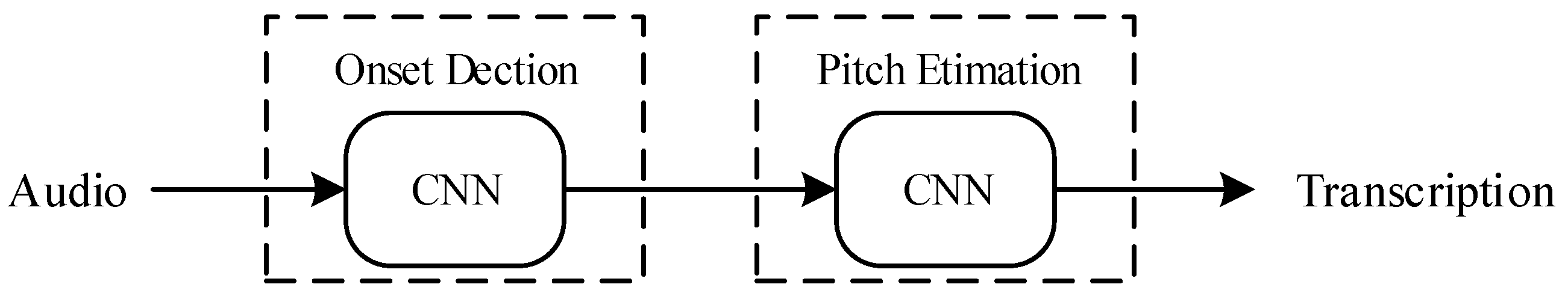
Here, we employ the hybrid note-based model in [21], which contains an onset detection module and a pitch estimation module. As shown in Figure 2, one CNN is used to detect onsets, and another CNN is used to estimate the probabilities of pitches at each detected onset.

We trained a CNN with one output unit as the onset detector, giving binary labels to distinguish onsets from non-onsets. The CNN takes a spectrogram slice of several frames as a single input, and each spectrogram excerpt centers on the frame to be detected. Feeding the spectrograms of the test signal to the network, we can obtain an onset activation function over time. The frame whose activation function is greater than the threshold is set as the detected onset.

The onset detector is followed by another CNN for multi-pitch estimation (MPE), which has the same architecture except for the output layer. Its input is a spectrogram slice centered at the onset frame. The CNN has 88 units in the output layer, corresponding to the 88 pitches of the piano. To make sure the multiple pitches can be estimated at the same time, all the outputs are transformed by a sigmoid function. In this case, a set of probabilities of 88 pitches at detected onsets is estimated through this network.

3.2. Integrated Architecture

The integrated architecture is constructed by applying the model in [27,28] to the note-level transcription. The model produces a posterior probability $p\left(\mathbf{y}\right|\mathbf{x})$, which can be represented using Bayes’ rule:

$$p\left(\mathbf{y}\right|\mathbf{x})=p(\mathbf{x}\left|\mathbf{y}\right)p\left(\mathbf{y}\right)/p\left(\mathbf{x}\right)$$

(10)

where $p\left(\mathbf{x}\right)$ and $p\left(\mathbf{y}\right)$ are the priors and $p\left(\mathbf{x}\right|\mathbf{y})$ is the likelihood of the sequence of acoustic inputs $\mathbf{x}$ and corresponding transcriptions $\mathbf{y}$. The likelihood can be factorized as follows:

$$p\left(\mathbf{x}\right|\mathbf{y})=p\left(x_1\right|\mathbf{y})\prod _{n=2}^{N}p\left(x_n\right|x_{t<n},\mathbf{y})$$

(11)

Similarly to the assumptions in HMMs, the following independence assumptions are made:

$$p\left(x_n\right|x_{\tau <n},\mathbf{y})=p\left(x_n\right|y_n)$$

(12)

$$p\left(\mathbf{x}\right)=\prod _{n=1}^{N}P\left(x_n\right)$$

(13)

Under these assumptions, the probability in Equation (11) can be written as:

$$\begin{array}{cc}\hfill p\left(\mathbf{x}\right|\mathbf{y})& =\prod _{n=1}^{N}p\left(x_n\right|y_n)\hfill \\ \hfill & =p\left(\mathbf{x}\right)\prod _{n=1}^{N}p\left(y_n\right|x_n)/p\left(y_n\right)\hfill \end{array}$$

(14)

Based on Equations (10) and (14), the posterior probability produced by the integrated architecture can be reformulated as follows:

$$p\left(\mathbf{y}\right|\mathbf{x})=p\left(\mathbf{y}\right)\prod _{n=1}^{N}p\left(y_n\right|x_n)/p\left(y_n\right)$$

(15)

where $p\left(y_n\right)$ is prior statistics analyzed on the training data. In Equation (15), the term $p\left(y_n\right|x_n)$ is obtained from the acoustic model, while the prior $p\left(\mathbf{y}\right)$ can be calculated from the MLM using Equation (1). Therefore, the acoustic model and the MLM are combined directly in the integrated architecture.

3.3. Inference Algorithm

The integrated model can be trained by maximizing the posterior of training sequences. The process is easy because training of the acoustic model and the MLM is independent. In the test stage, we also aim to find the note sequence $\mathbf{y}$ maximizing the posterior $p\left(\mathbf{y}\right|\mathbf{x})$, which can be reformulated as a recursive form:

$$p\left(y_{\tau <n+1}\right|x_{\tau <n+1})=p\left(y_{\tau <n}\right|x_{\tau <n})p\left(y_n\right|y_{\tau <n})p\left(y_n\right|x_n)/p\left(y_n\right)$$

(16)

However, the test inference is rather complex. To estimate $y_n$ in the note sequence, we need to know the history $y_{\tau <n}$ and the acoustic output $p\left(y_n\right|x_n)$. Here, the history $y_{\tau <n}$ is not determined, and the possible configurations of $y_n$ are exponential in the number of pitches. Therefore, greedily searching for the best solution of $\mathbf{y}$ is intractable.

Beam search is an algorithm for decoding, which is commonly used in speech recognition. There are two parameters when it scales to note sequences: K is the branching factor, and w is the width of the beam. The algorithm considers only K most possible configurations of $y_n$ according to the acoustic output $p\left(y_n\right|x_n)$. At each inference step, no more than w partial solutions are maintained for further search. As shown in Equation (16), the K candidates for $y_n$ should be configurations maximizing $p\left(y_n\right|y_{\tau <n})p\left(y_n\right|x_n)/p\left(y_n\right)$, and w is the number of partial solutions maximizing $p\left(y_{\tau <n+1}\right|x_{\tau <n+1})$ or $p\left(y_{\tau <n}\right|x_{\tau <n})$.

Similar to the frame-based inference in [30], the beam search algorithm can be used to decode globally using the raw outputs of the note-based acoustic model and the MLM. This method will be referred to as global beam search (GBS). As described in Algorithm 1, the K candidates at each onset are sampled from the posterior probability $p\left(y_n\right|x_n)$. The simplified process is effective because the possible configurations of $y_n$ can be easily enumerated through the independent acoustic outputs.

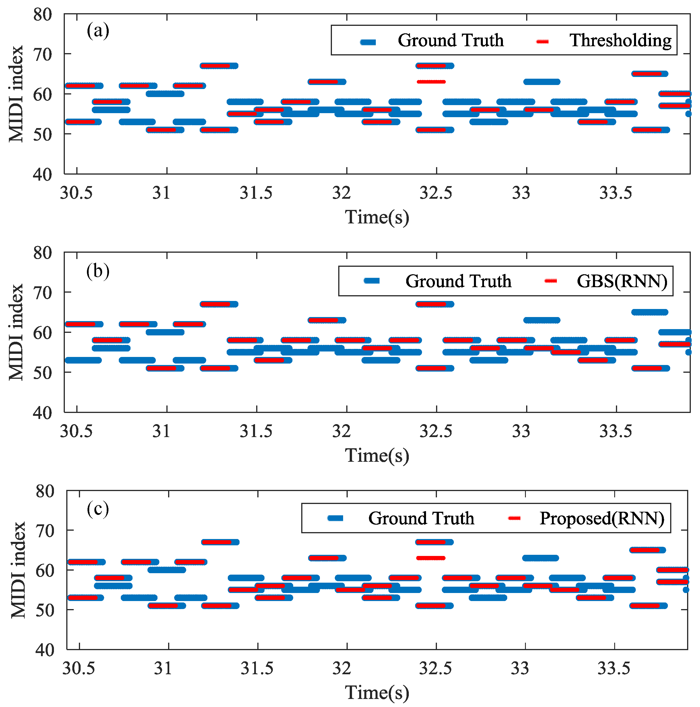
In the proposed inference algorithm (Algorithm 2), we adopt the beam search algorithm to repair the thresholding transcription results locally. Applying a proper threshold to the acoustic outputs, the note-based acoustic model produces a preliminary transcription. However, the fixed threshold leads to some false negative notes at the detected onset. Rather than decoding at each onset of the note sequence, the beam search algorithm is used to predict notes only at the blank onsets. At the non-blank onset, $y_n$ is determined through applying a threshold to the pitch probabilities $p\left(y_n\right|x_n)$. The determined notes without using MLM could avoid the accumulation of mistakes in a sequence over time. At each blank onset, we choose the top K candidates for $y_n$ maximizing $p\left(y_n\right|x_n)$. Under the rule of maximizing the posterior $p\left(\mathbf{y}\right|\mathbf{x})$, notes at the blank onsets are predicted using the context information.

Algorithm 1 Global beam search (GBS).

Input: The acoustic model’s outputs $p_a\left(y_n\right|x_n)$ at onset $n\in [1,N]$;            The beam width w; the branching factor K. Output: The most likely note sequence $\mathbf{y}=y_{\tau \le N}$.  beam${}^{*}$← new beam object  beam.insert$(0,\left\{\right\},m_{ml})$  for $n=1$ to N do   beam_tmp ← new beam object   for $l,s,m_{ml}$ in beam do    for $k=1$ to K do     $y^{\prime }=p_a\left(y_n\right|x_n).k$-th_most_probable()     $l^{\prime }=log{p}_{ml}\left(y^{\prime }\right|s)+log{p}_a\left(y^{\prime }\right|x_n)-logp\left(y^{\prime }\right)$     $m_{ml}^{\prime }\leftarrow m_{ml}$ with $y_n:=y^{\prime }$     beam_tmp.insert$(l+l^{\prime },\{s,y^{\prime }\},m_{ml}^{\prime })$    end for   end for   beam_tmp ← min-priority queue of capacity $w^{**}$   beam ← beam_tmp  end for  return beam.pop() * Beam object is a queue of triple $\{l,s,m_{ml}\}$, where at onset n, l is the accumulated posterior probability $p\left(y_{\tau <n}\right|x_{\tau <n})$, s is the partial candidate note sequence $y_{\tau <n}$ and $m_{ml}$ stands for the music language model taking $y_{\tau <n}$ as the current input. $**$ A min-priority queue of fixed capacity w maintains at most w highest values.

Algorithm 2 Local beam search (LBS).

Input: The acoustic model’s outputs $p_a\left(y_n\right|x_n)$ at onset $n\in [1,N]$; The beam width w;            The branching factor K; the threshold T applied to the acoustic outputs. Output: The most likely note sequence $\mathbf{y}=y_{\tau \le N}$.  beam${}^{*}$← new beam object  beam.insert$(0,\left\{\right\},m_{ml})$  for $n=1$ to N do   beam_tmp ← new beam object   for $l,s,m_{ml}$ in beam do    $y^{\prime }=p_a\left(y_n\right|x_n).$exceed the threshold T    if $y^{\prime }.$isEmpty() then     for $k=1$ to K do      $y^{″}=p_a\left(y_n\right|x_n).k$-th_probable()      $l^{\prime }=log{p}_{ml}\left(y^{″}\right|s)+log{p}_a\left(y^{″}\right|x_n)-logp\left(y^{″}\right)$      $m_{ml}^{\prime }\leftarrow m_{ml}$ with $y_n:=y^{″}$      beam_tmp.insert$(l+l^{\prime },\{s,y^{″}\},m_{ml}^{\prime })$     end for    else     $l^{\prime }=log{p}_{ml}\left(y^{\prime }\right|s)+log{p}_a\left(y^{\prime }\right|x_n)-logp\left(y^{\prime }\right)$     $m_{ml}^{\prime }\leftarrow m_{ml}$ with $y_n:=y^{\prime }$     beam_tmp.insert$(l+l^{\prime },\{s,y^{\prime }\},m_{ml}^{\prime })$    end if   end for   beam_tmp ← min-priority queue of capacity $w^{**}$   beam ← beam_tmp  end for  return beam.pop() * Beam object is a queue of triple $\{l,s,m_{ml}\}$, where at onset n, l is the accumulated posterior probability $p\left(y_{\tau <n}\right|x_{\tau <n})$, s is the partial candidate note sequence $y_{\tau <n}$ and $m_{ml}$ stands for the music language model taking $y_{\tau <n}$ as the current input. $**$ A min-priority queue of fixed capacity w maintains at most w highest values.

4. Experiments

4.1. Dataset

The experiments are conducted on the MAPS database [31]. It is a complete piano dataset that contains audio recordings, related aligned MIDI files and annotated text files. There are nine categories of recordings corresponding to different piano types and recording conditions. Each category consists of isolated notes, chords and 30 pieces of music.

In the transcription experiments, we only use the full music pieces in MAPS and divide them into training, validation and test splits. To evaluate the performance of the MLM, the training data and test data contain no overlapping contents. Here, we choose the categories “StbgTGd2” and “ENSTDkCl” as the test set, which consists of 60 musical pieces. Category “StbgTGd2” is produced by the default software piano synthesizer, and “ENSTDkCl” is obtained from a real Yamaha Disklavier upright piano. In the other seven categories of MAPS, there are 179 pieces of music, which are different from the contents in test data. For these 179 pieces, we select 90% for training (161 pieces) and the remaining 10% for validation (18 pieces). Details for the data partitions are presented in Appendix.

To evaluate the proposed system, we also use the whole LabROSA piano transcription dataset as another test set [22]. There are 29 pieces of music in this database, along with aligned MIDI files. The MIDI data are collected from Piano-midi.de, and piano recordings are made using a Yamaha Disklavier playback grand piano.

4.2. Experimental Settings

The acoustic model takes the spectrograms of CQT as input. The audio signal is segmented with a frame length of 100 ms and a hop size of 10 ms. A context window of nine frames is applied to the 267 dimensional CQTs so that we could obtain a spectrogram slice. The two CNNs have the same structure, except for the output layer. The model configurations for the CNNs are presented in

Table 1. Model configuration for the CNNs.

Type	Patch Size/Stride	Input Size
Conv 1	16 × 2/1	267 × 9
Pool 1	2 × 2/2	252 × 8 × 10
Conv 2	11 × 3/1	126 × 4 × 10
Pool 2	2 × 2/2	116 × 2 × 20
Fully-connected	256	58 × 1 × 20

. For the spectrogram slices of $267\times 9$, the first convolutional layer with 10 filters of size $16\times 2$ computes 10 feature maps of size $252\times 8$. The next layer performs max-pooling of $2\times 2$, reducing the size of maps to $126\times 4$. The second convolutional layer contains 20 filters of size $11\times 3$, and the max-pooling size of the second pooling layer is also set to $2\times 2$. The fully-connected layer contains 256 units, and the number of units in the output layer changes with the task. In the CNN for onset detection, the output layer has a single unit. In the CNN for multi-pitch estimation, the output layer has 88 units and employs the sigmoid as the activation function to yield 88 independent pitch probabilities. The CNNs were trained using mini-batch gradient descent with size 256. The Adam algorithm was used in the training [32]. An initial learning rate of 0.01 was decreased to zero over 100 epochs. To prevent over-fitting, a dropout of 0.5 was applied to each network. We also used the method of early stopping, in which training was stopped if the cost (cross entropy) did not decrease for 20 epochs.

As mentioned in Section 2, we take the RNN, RNN-RBM and their LSTM variants as MLMs. Both the RNN and LSTM have one single hidden layer, which contains 100 hidden nodes. In the RNN-RBM or LSTM-RBM, the number of recurrent hidden nodes is also 100, and the RBM has 50 hidden units. The training pieces are divided into sub-sequences of length 20. All these MLMs were trained using the note sequences by back-propagation through time (BPTT). We used mini-batch of size 100 and the Adam algorithm for gradient updating. The initial learning rate was set to 0.01, which was linearly reduced to zero over 100 iterations. In addition to dropout, we also adopted early stopping to prevent over-fitting.

Note-based metrics are employed to assess the performance of the proposed system. A note event is regarded as right if its pitch is correct and its onset is within a $\pm 50$ ms range of the ground truth onset. These measures are defined as:

$$P=\frac{N_{TP}}{N_{TP}+N_{FP}}$$

(17)

$$R=\frac{N_{TP}}{N_{TP}+N_{FN}}$$

(18)

$$F=\frac{2\ast P\ast R}{P+R}$$

(19)

where P, R, F correspond to the precision, recall and F-measure, respectively, and $N_{TP}$, $N_{FP}$ and $N_{FN}$ are the numbers of true positives, false positives and false negatives, respectively.

4.3. Results

The transcription experiments are performed with various configurations. The CNN-based acoustic model yields a sequence of probabilities for 88 individual pitches, and various post-processing methods are used to transform the probabilities into binary notations. The first method is simplest, which applies a threshold to the acoustic outputs. We select the threshold that maximizes the F-measure over the validation set and use the threshold of 0.5 for the following testing. In the proposed architecture, the other two methods are implemented using simple RNN MLMs. As mentioned in Section 3, the GBS algorithm searches for the partial solutions at each detected onset, whereas the proposed inference algorithm predicts notes only at the blank onsets in the thresholding transcription results.

Experimental results on the software piano “StbgTGd2” are presented in

Table 2. Transcription results on the software piano “StbgTGd2”. GBS, global beam search.

Post-Processing	Recall	Precision	F-Measure
Thresholding	0.8839	0.9169	0.9001
GBS (RNN)	0.8592	0.9184	0.8878
Proposed (RNN)	0.8946	0.9111	0.9027

. In Table 2, we display the note-based recall, precision and F-measure for systems using the three post-processing methods. The acoustic model with the simplest thresholding yields a high F-measure over 90%, which indicates that the CNNs are effective in onset detection and multi-pitch estimation. Compared with the thresholding method, the global decoding post-processing of GBS results in worse transcription on the F-measure. The transcriptions produced by the GBS contain fewer notes, so the recall is lower than that of the thresholding results. This is probably due to the MLM, which is trained to predict notes using the true history. In the GBS algorithm, we take the previous w candidate solutions as the history, which are estimated using outputs of the acoustic model and the MLM. The drawback of prediction accumulates over time, so that the performance of transcription is unsatisfactory. The proposed algorithm yields a better performance than the GBS on the recall and F-measure, since the determined notes at non-blank onsets can help reduce the accumulation of errors. The improvement of recall is at the cost of a loss of precision. The proposed algorithm also outperforms the thresholding method on recall, which illustrates that the note-based MLM could model note sequences to some extent.

Table 3. Transcription results on the real piano “ENSTDkCl”.

Post-Processing	Recall	Precision	F-Measure
Thresholding	0.6765	0.8115	0.7374
GBS (RNN)	0.6693	0.7919	0.7225
Proposed (RNN)	0.6991	0.7942	0.7436

displays the transcription results on the real piano “ENSTDkCl”. As shown in Table 2, a similar trend can be seen in Table 3, where the best performance is achieved using the proposed algorithm. All the note-based metrics in Table 3 are worse than those in Table 2. This is because the notes produced by the real piano are not as regular as the notes from the software. Additionally, there are some deviations and noises when the real piano is played. Therefore, there are many accumulated errors in the decoding of GBS. This partly explains why the GBS generates the worst results on all metrics.

Table 4. Transcription results on the real piano of LabROSA.

Post-Processing	Recall	Precision	F-Measure
Thresholding	0.4667	0.7688	0.5884
GBS (RNN)	0.4507	0.7352	0.5626
Proposed (RNN)	0.5368	0.7101	0.6114

presents the transcription results on the LabROSA dataset of real piano recordings. In Table 4, the differences between the results of these three post-processing methods are obvious. We can draw the same conclusion that the proposed inference algorithm improves the performance of transcription using the RNN MLM.

Figure 3 shows the threshold’s influence on the performance of the thresholding method and proposed algorithm. The threshold of 0.5 is reasonable for the three test sets. We also observe that the performance difference between the thresholding method and the proposed algorithm increases with the increase of the threshold. A higher threshold value will bring more blank onsets, so the superiority of the proposed algorithm for the thresholding method is more obvious. Through Table 2, Table 3 and Table 4 and Figure 3, we also observe that the superiority of the proposed algorithm compared to the other two methods is more obvious when the acoustic model has a poorer performance in transcription. At the threshold of 0.5, we further perform a paired t-test over 10-fold cross-validation on the MAPS dataset. The t-test is used to check whether the proposed algorithm outperforms the thresholding on the F-measure. The p-value of 0.0472 demonstrates that the improvement of the proposed algorithm over the thresholding method is statistically significant.

Figure 4 shows the transcriptions of the three post-processing methods along with the corresponding ground truth piano roll. The excerpt is a part of track bach_847MINp_align in the LabROSA dataset. As shown in the ground truth, the polyphony at each time is two. In the results of thresholding, there are five blank onsets from 31.9 s–33.3 s. From the bottom subfigure, we can see that the proposed algorithm predicts notes at these five onsets. Although there is no blank onset in the results of GBS, some notes could not be predicted. For example, compared with the other two subfigures, there are false negative notes at the first and the last two onsets in the middle subfigure. This example demonstrates that the proposed algorithm can achieve better performance than other two post-processing methods.

To further evaluate the performance of note-based MLMs, more transcription experiments are conducted using the proposed inference algorithm.

Table 5. Results for MLMs on the software piano “StbgTGd2”. MLM, music language model.

MLM	Recall	Precision	F-Measure
RNN	0.8946	0.9111	0.9027
RNN-RBM	0.8954	0.9112	0.9032
LSTM	0.8948	0.9114	0.9030
LSTM-RBM	0.8960	0.9112	0.9035

presents the transcription results of software piano “StbgTGd2”. As shown in Table 5, the performance is improved slightly when we replace the RNN cells with LSTM cells in the MLMs. This is largely attributed to the fact that the LSTM could model longer term dependencies in note sequences than RNN. The RBM-based joint models outperform the single RNN or LSTM, which indicates that combining the RBM and recurrent structure as the MLM can estimate high-dimensional, temporal distributions better.

The evaluation results on the real piano “ENSTDkCl” are displayed in

Table 6. Results for MLMs on the real piano “ENSTDkCl”.

MLM	Recall	Precision	F-Measure
RNN	0.6991	0.7942	0.7436
RNN-RBM	0.6999	0.7952	0.7445
LSTM	0.6991	0.7940	0.7435
LSTM-RBM	0.7009	0.7952	0.7451

correspondingly. Adding RBM to the RNN or LSTM improves the MLM’s performance in all respects. However, the LSTM has no superiority over RNN without the RBM. The main reason is that the acoustic model achieves a poor performance on transcribing the real piano. In this case, there are many errors in the thresholding results or history solutions. Therefore, the LSTM’s advantage of longer memory does not work here. The combination of RBM and LSTM can alleviate the problem because the distribution estimator RBM has the attribution of denoising.

Table 7. Results for MLMs on the real piano of LabROSA.

MLM	Recall	Precision	F-Measure
RNN	0.5368	0.7101	0.6114
RNN-RBM	0.5371	0.7105	0.6117
LSTM	0.5339	0.7063	0.6082
LSTM-RBM	0.5377	0.7108	0.6123

shows the transcription results of the LabROSA dataset. As shown in Table 6, similar results can be seen in Table 7 where the best performance is achieved by the LSTM-RBM. We also observe the differences between the results of LSTM and other MLMs. In the results of thresholding, the error rate is rather high. Therefore, the LSTM accumulates more errors than RNN and leads to the worst performance.

5. Conclusions

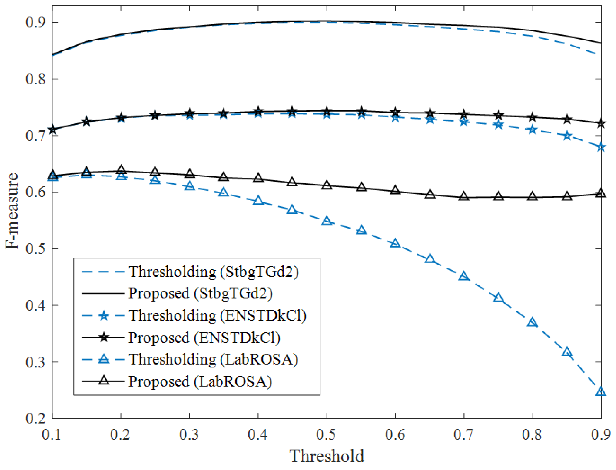
In this paper, we propose note-based MLMs for modeling note-level music structure. These note-based MLMs are trained to predict notes at the next onset, which is different from the smoothing operation of existing frame-based MLMs. An integrated architecture is used to combine the outputs of the MLM and the note-based acoustic model directly. We also propose an inference algorithm, which uses the note-based MLM to predict notes at the blank onsets in the thresholding transcription results. The experiments are conducted on the MAPS and LabROSA databases. Although the proposed algorithm only achieves an absolute 0.34% F-measure improvement on the synthetic data, it reaches absolute 0.77% and 2.39% improvements on two real piano test sets, respectively. We also observe that the combination of RBM and recurrent structure models the high-dimensional sequences better than a single RNN or LSTM does. Although the LSTM shows no superiority to other MLMs in transcribing the real piano, the LSTM-RBM always helps the system yield the best results regardless of the performance of acoustic models.

Overall, the improvement of the proposed algorithm over the thresholding method is small. One of the possible reasons is the limited training data. The MLMs are trained using only 161 pieces in the MAPS database, and the small amount of data may lead the neural networks to over-fitting. The abundance of musical scores can provide a way to solve the problem. Besides, the note sequences are indexed using the onset in the current system. Actually, the temporal structure of musical sequences should contain how the notes appear and last correlatively. Ignoring the note’s offset or duration time, the representation of musical sequences is partial. Therefore, the MLMs in this paper cannot model the temporal structure of note sequences completely. In the future, we will search for a proper way to represent the note-level musical sequences. One possible solution is to add a duration model to the current MLMs, such as an HMM.

References

1. Moorer, J.A. On the transcription of musical sound by computer. Comput. Music J. 1977, 1, 32–38. [Google Scholar]
2. Klapuri, A. Introduction to music transcription. In Signal Processing Methods for Music Transcription; Springer: New York, NY, USA, 2006; pp. 3–20. [Google Scholar]
3. Cogliati, A.; Duan, Z.; Wohlberg, B. Piano transcription with convolutional sparse lateral inhibition. IEEE Signal Process. Lett. 2017, 24, 392–396. [Google Scholar]
4. Benetos, E.; Dixon, S.; Giannoulis, D.; Kirchhoff, H.; Klapuri, A. Automatic music transcription: Challenges and future directions. J. Intell. Inform. Syst. 2013, 41, 407–434. [Google Scholar] [CrossRef]
5. Klapuri, A.P. Multiple fundamental frequency estimation based on harmonicity and spectral smoothness. IEEE Trans. Speech Audio Process. 2003, 11, 804–816. [Google Scholar] [CrossRef]
6. Pertusa, A.; Inesta, J.M. Multiple fundamental frequency estimation using Gaussian smoothness. In Proceedings of the IEEE International Conference on Acoustics, Speech and Signal Processing (ICASSP), Las Vegas, NV, USA, 31 March–4 April 2008; pp. 105–108. [Google Scholar]
7. Brown, J.C. Calculation of a constant Q spectral transform. J. Acoust. Soc. Amer. 1991, 89, 425–434. [Google Scholar] [CrossRef]
8. Smaragdis, P.; Brown, J.C. Non-negative matrix factorization for polyphonic music transcription. In Proceedings of the IEEE Workshop on Applications of Signal Processing to Audio and Acoustics, New Paltz, NY, USA, 19–22 October 2003; pp. 177–180. [Google Scholar]
9. Smaragdis, P.; Raj, B.; Shashanka, M. A probabilistic latent variable model for acoustic modeling. Adv. Models Acoust. Process. 2006, 148. [Google Scholar]
10. Benetos, E.; Dixon, S. A shift-invariant latent variable model for automatic music transcription. Comput. Music J. 2012, 36, 81–94. [Google Scholar]
11. Nam, J.; Ngiam, J.; Lee, H.; Slaney, M. A classification-based polyphonic piano transcription approach using learned feature representations. In Proceedings of the International Society for Music Information Retrieval Conference (ISMIR), Miami, FL, USA, 24–28 October 2011; pp. 175–180. [Google Scholar]
12. Böck, S.; Schedl, M. Polyphonic piano note transcription with recurrent neural networks. In Proceedings of the IEEE International Conference on Acoustics, speech and signal processing (ICASSP), Kyoto, Japan, 25–30 March 2012; pp. 121–124. [Google Scholar]
13. Kelz, R.; Widmer, G. An experimental analysis of the entanglement problem in neural-network-based music transcription systems. Proceedings of AES Conference on Semantic Audio, Erlangen, Germany, 22–24 June 2017. [Google Scholar]
14. Berg-Kirkpatrick, T.; Andreas, J.; Klein, D. Unsupervised transcription of piano music. In Proceedings of the International Conference on Neural Information Processing Systems, Montreal, QC, Canada, 8–13 Demcember 2014; pp. 1538–1546. [Google Scholar]
15. Ewert, S.; Plumbley, M.D.; Sandler, M. A dynamic programming variant of non-negative matrix deconvolution for the transcription of struck string instruments. In Proceedings of the IEEE International Conference on Acoustics, Speech and Signal Processing (ICASSP), Brisbane, QLD, Australia, 19–24 April 2015; pp. 569–573. [Google Scholar]
16. Kameoka, H.; Nishimoto, T.; Sagayama, S. A multipitch analyzer based on harmonic temporal structured clustering. IEEE Tran. Audio Speech Lang. Process. 2007, 15, 982–994. [Google Scholar] [CrossRef]
17. Cogliati, A.; Duan, Z. Piano music transcription modeling note temporal evolution. In Proceedings of the IEEE International Conference on Acoustics, Speech and Signal Processing (ICASSP), Brisbane, QLD, Australia, 19–24 April 2015; pp. 429–433. [Google Scholar]
18. Cogliati, A.; Duan, Z.; Wohlberg, B. Context-dependent piano music transcription with convolutional sparse coding. IEEE/ACM Trans. Audio Speech Lang. Process. 2016, 24, 2218–2230. [Google Scholar] [CrossRef]
19. Cheng, T.; Mauch, M.; Benetos, E.; Dixon, S. An attack/decay model for piano transcription. In Proceedings of the International Society for Music Information Retrieval Conference (ISMIR), NY, USA, 7–11 August 2016. [Google Scholar]
20. Costantini, G.; Perfetti, R.; Todisco, M. Event based transcription system for polyphonic piano music. Signal Process. 2009, 89, 1798–1811. [Google Scholar] [CrossRef]
21. Wang, Q.; Zhou, R.; Yan, Y. A two-stage approach to note-level transcription of a specific piano. Appl. Sci. 2017, 7, 901. [Google Scholar] [CrossRef]
22. Poliner, G.E.; Ellis, D.P. A discriminative model for polyphonic piano transcription. EURASIP J. Appl. Signal Process. 2007, 2007, 154. [Google Scholar] [CrossRef]
23. Raczyński, S.A.; Vincent, E.; Sagayama, S. Dynamic Bayesian networks for symbolic polyphonic pitch modeling. IEEE Trans. Audio Speech Lang. Process. 2013, 21, 1830–1840. [Google Scholar] [CrossRef]
24. Boulanger-Lewandowski, N.; Bengio, Y.; Vincent, P. Modeling temporal dependencies in high-dimensional sequences: Application to polyphonic music generation and transcription. In Proceedings of the 29th International Conference on Machine Learning (ICML), Edinburgh, Scotland, 27 June–3 July 2012; pp. 1159–1166. [Google Scholar]
25. Boulanger-Lewandowski, N.; Bengio, Y.; Vincent, P. High-dimensional sequence transduction. In Proceedings of the 2013 IEEE International Conference on Acoustics, Speech and Signal Processing (ICASSP), Vancouver, BC, Canada, 26–31 May 2013; pp. 3178–3182. [Google Scholar]
26. Sigtia, S.; Benetos, E.; Cherla, S.; Weyde, T.; Garcez, A.; Dixon, S. RNN-based music language models for improving automatic music transcription. In Proceedings of the International Society for Music Information Retrieval Conference (ISMIR), Taipei, Taiwan, 27–31 October 2014. [Google Scholar]
27. Sigtia, S.; Benetos, E.; Boulanger-Lewandowski, N.; Weyde, T.; Garcez, A.S.D.; Dixon, S. A hybrid recurrent neural network for music transcription. In Proceedings of the IEEE International Conference on Acoustics, Speech and Signal Processing (ICASSP), Brisbane, QLD, Australia, 19–24 April 2015; pp. 2061–2065. [Google Scholar]
28. Sigtia, S.; Benetos, E.; Dixon, S. An end-to-end neural network for polyphonic piano music transcription. IEEE/ACM Trans. Audio Speech Lang. Process. 2016, 24, 927–939. [Google Scholar] [CrossRef]
29. Ycart, A.; Benetos, E. A study on LSTM networks for polyphonic music sequence modelling. In Proceedings of the International Society for Music Information Retrieval Conference (ISMIR), Suzhou, China, 23–28 October 2017. [Google Scholar]
30. Sigtia, S.; Boulanger-Lewandowski, N.; Dixon, S. Audio chord recognition with a hybrid recurrent neural network. In Proceedings of the International Society for Music Information Retrieval Conference (ISMIR), Malaga, Spain, 26–20 October 2015. [Google Scholar]
31. Emiya, V.; Badeau, R.; David, B. Multipitch estimation of piano sounds using a new probabilistic spectral smoothness principle. IEEE Trans. Audio Speech Lang. Process. 2010, 18, 1643–1654. [Google Scholar] [CrossRef]
32. Kingma, D.; Ba, J. Adam: A method for stochastic optimization. arXiv, 2014; arXiv:1412.6980. [Google Scholar]
Figure 1. The graphical structure of RNN-RBM.
Applsci 08 00470 g001
Figure 2. Diagram for the note-based acoustic model.
Applsci 08 00470 g002
Figure 3. F-measure on the three test sets as a function of the threshold.
Applsci 08 00470 g003
Figure 4. Binary piano-roll transcription of an example track obtained through the thresholding method (a), the GBS algorithm (b) and the proposed Local beam search (LBS) algorithm (c).
Applsci 08 00470 g004