An Investigation of the High Efficiency Estimation Approach of the Large-Scale Scattered Point Cloud Normal Vector

Abstract

The normal vector estimation of the large-scale scattered point cloud (LSSPC) plays an important role in point-based shape editing. However, the normal vector estimation for LSSPC cannot meet the great challenge of the sharp increase of the point cloud that is mainly attributed to its low computational efficiency. In this paper, a novel, fast method-based on bi-linear interpolation is reported on the normal vector estimation for LSSPC. We divide the point sets into many small cubes to speed up the local point search and construct interpolation nodes on the isosurface expressed by the point cloud. On the premise of calculating the normal vectors of these interpolated nodes, a normal vector bi-linear interpolation of the points in the cube is realized. The proposed approach has the merits of accurate, simple, and high efficiency, because the algorithm only needs to search neighbor and calculates normal vectors for interpolation nodes that are usually far less than the point cloud. The experimental results of several real and simulated point sets show that our method is over three times faster than the Elliptic Gabriel Graph-based method, and the average deviation is less than 0.01 mm.

1. Introduction

With the popularity of 3D scanning measurement technology, the acquisition of large-scale scattered point cloud (LSSPC) is easier due to the high resolution of the scanning devices. However, the point based model must be processed for rendering, feature recognition, smoothing, sampling, and surface reconstruction to meet the requirements of the application. The normal vector estimation is actually the basis of point cloud editing, while the efficiency barely meets the great demand of the application.

Many algorithms aim to estimate the normal vectors of the scattered point cloud. The Euclidean nearest neighbor (ENN)-based methods are the most popular algorithms due to their simplicity [1,2]. Cao [3] presented a fast and quality estimator based on a neighborhood shift to estimate the normal vector accurately. Hotta and Iwakiri [4] realized 3D point cloud cluster analysis using the Principal Component Analysis (PCA) of normal vector distribution that depends on a neighbor. Ouyang and Feng [5] developed a method based on fitted directional tangent vectors using a local voronoi mesh, which needs to identify the neighboring points first. Park [6] focused on finding balanced neighbors using an Elliptic Gabriel graph (EGG) algorithm, followed by local quadratic surface fitting methods for the normal vector estimation of each point. Zhang [7] reported a low-rank subspace clustering algorithm to estimate the normal vector robustly, while the method had to distinguish whether the points belonged to smooth regions and calculate the normal vector for them before clustering. The calculation of normal vectors based on ENN usually performs the following steps: First, sort the scattered point cloud into a classic data structure, such as a k-d tree [8] or hash table; then, search the nearest neighbor within a fixed quantity or a fixed distance of each point; at last, compute the normal vector using neighbor points for each point.

Although these ENN-based methods are widely used, there are some difficulties to overcome [9,10]. On one hand, the ENN is generally determined by a predefined constant or a spherical space with a specific radius. The reasonable neighborhood range is crucial for accurate and reliable normal vector estimation, especially when dealing with LSSPC [11]. On the other hand, these ENN-based algorithms are perhaps reasonable in the distance but are not reasonable in spatial distribution [12]. When the point distribution is uneven, the distance-based method gives obviously unbalanced neighbors, which result in unreliable normal vector estimation results. Park [6] and Lee [13] discussed the EGG algorithm that was used to overcome this shortcoming, but this EGG algorithm does not consider the situation that the point is located at the edge of the surface.

Some researchers use the triangle mesh to calculate the normal vector for the point cloud. Ma [14] introduced a new normal vector estimation method based on the matching results of the local Delaunay triangle mesh formed at each point. The normal vectors of the triangular meshes that contain the given point were recorded by local searching at first; then, the average of these normal vectors was calculated as the normal vector of the point. Chen and Wu [15] used the centered weights to approximate normal vectors. However, different triangulation results may lead to different normal vector calculation results due to the ambiguity when converting the point cloud to triangulation.

Either the ENN-based methods or the triangle-based algorithms—whichever is the nearest neighbor for each point—needs to be found. This means huge times of power operation, open square operation, and comparison operation are involved in neighbor searching. It is a very time-consuming process [16,17], especially when dealing with large-scale scattered point cloud. The hash table is widely used in the nearest neighbor searching [18], since hash tables turn out to be more efficient than search trees or any other look-up table structure in many situations [19,20]. However, it will dramatically reduce the efficiency when the density of point cloud is non-uniform. Some algorithms try to improve the nearest neighbor searching algorithm by sorting the distance from the point to an adjacent region; however, the effect of this is limited. Another algorithm that seriously affects efficiency is the singular value decomposition (SVD) of the covariance matrix, which was widely used in the normal vector calculation. Given an n order matrix, the SVD of the matrix takes O(n³) floating-point operations (flops) [21]. This will have a disastrous impact on the normal vector calculation, especially when the number of the point cloud is huge.

In this paper, it is the intention that a high efficiency estimation approach is proposed for the predicted normal vector of LSSPC. This algorithm takes three primary steps to compute the normal vector for each point, and it is described in detail in Section 2. In Section 3, the experiments are carried out, and the results are completely discussed.

2. Materials and Methods

2.1. The Interpolation Nodes and Nearest Neighbor

For an arbitrary point of point-based shape, the normal vector represents the tangent plane direction of the unknown isosurface. In order to calculate the normal vector for all points, we first construct the interpolation nodes and calculate the normal vector for these points based on Marching Cube algorithm, which was first developed as a result of the research on visualizing Computed Tomography data and Magnetic Resonance Imaging data [22].

Therefore, it is necessary to establish a spatial topology to speed up the local point cloud search. An automatic method was introduced to segment the point cloud into some small cubes, and then the hash table was established by assigning the indexes to these cubes.

Given a point set S = {X_t = (x_t, y_t, z_t)|t = 1, …, N}, in which N is the number of the point set. The efficiency and the accuracy were strongly associated with the cube’s size L. Small L means high accuracy, while larger L means high efficiency. According to the literature [23], a reasonable computation of L can be easily extended from 2D to 3D:

$$L=\sqrt[3]{\frac{(x_{\max }-x_{\min })\times (y_{\max }-y_{\min })\times (z_{\max }-z_{\min })}{N}}$$

(1)

in which x_max, x_min, y_max, y_min, z_max, z_min are the maximum and minimum values of point cloud along the X, Y, and Z axes, respectively.

Once the size of the cube is determined, the total number of the cubes index_i, index_j, and index_k were calculated separately according to X, Y, and Z axes.

$$\{\begin{array}{l}inde{x}_i=(x_{\max }-x_{\min })/L\\ inde{x}_j=(y_{\max }-y_{\min })/L\\ inde{x}_k=(z_{\max }-z_{\min })/L\end{array}$$

(2)

The cube contains the point X_t = (x_t, y_t, z_t) can be indexed with:

$$\{\begin{array}{l}i=(x_t-x_{\min })/L\\ j=(y_t-y_{\min })/L\\ k=(z_t-z_{\min })/L\end{array}$$

(3)

Then the point X_t can be mapped to hash table by the following hash function:

$$key=inde{x}_i\times inde{x}_j\times k+inde{x}_i\times j+i$$

(4)

This is a process of projection and quantization that places each point in a cube indexed with (i, j, k) that can correspond to the integer key through the hash function.

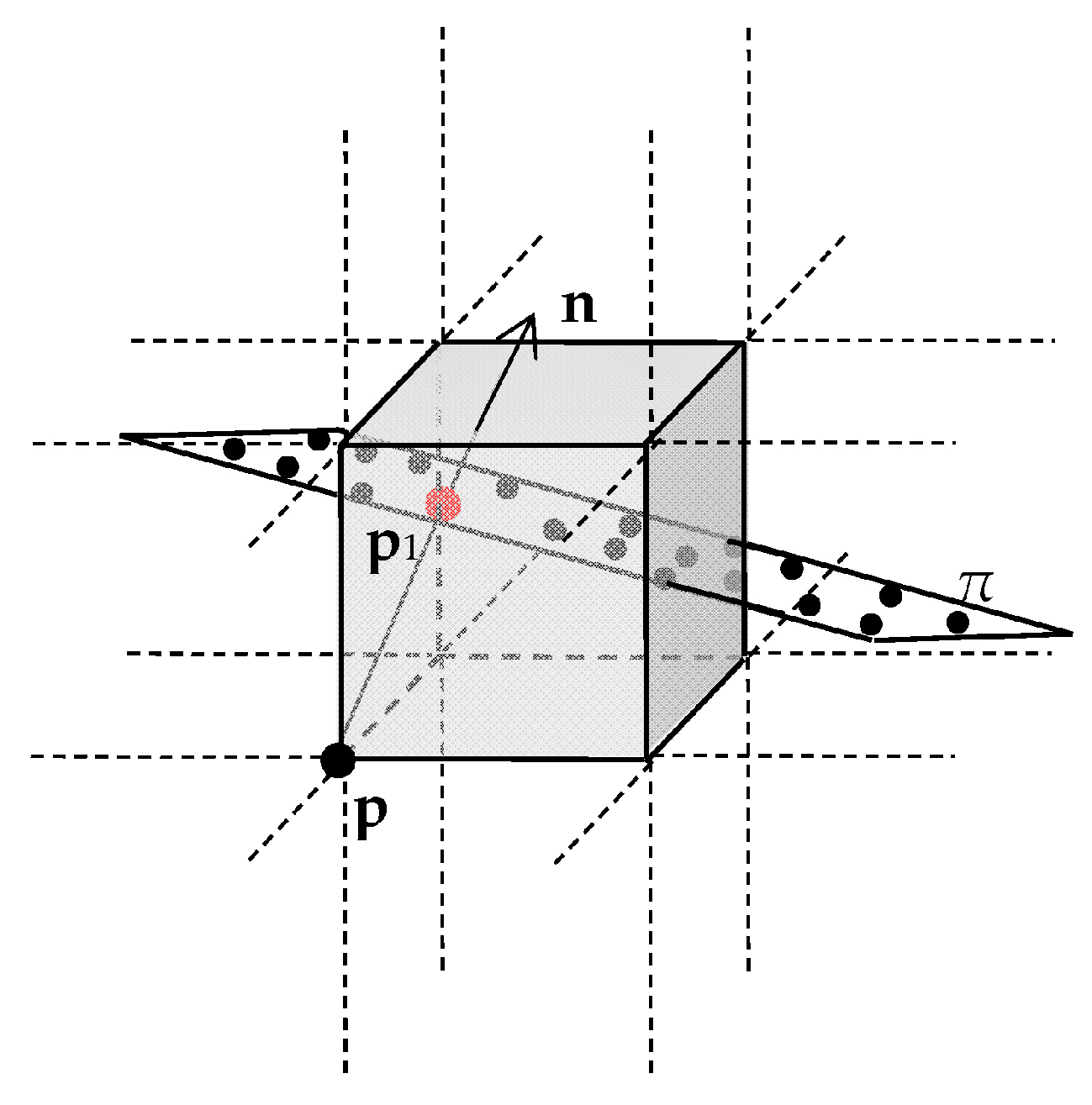
Given a cube with an index of (i, j, k), the Marching Cubes algorithm calculates a signed distance for all eight vertices of each cube; then, the intersection points of the cube’s edges and the unknown isosurface is calculated according to these signed distances of the vertex [24]. Since the normal vector of the point cloud is unknown, the signed distance cannot be calculated, so the coordinates of the intersection points cannot be obtained. However, we can project the grid point p to the tangent plane of the unknown isosurface to get the projection points p₁ in Figure 1. We call the projection points p₁ an interpolation node.

The randomness of scattered point cloud leads to the fact that the neighborhood of a point is generally not symmetric. The normal vector of the same point will change according to the change of the neighborhood range. We avoid this problem by searching the given cube and the 26 surrounding cubes and get all the neighborhood points of the geometric center point p.

When the cube is small enough, it is considered that the points in a cube are on the same tangent plane and have nearly the same normal vector n. Figure 1 shows that the vertex point p is usually not on the unknown isosurface; it can be projected to the surface along the direction of the normal vector n that is defined by the neighbor of point p. The interpolation node p₁ is on the tangent plane π. The Euclidean distance from p to p₁ is the smallest, and the neighbor of the p can be regarded as the neighbor of p₁; then, the p₁ shares the normal vector n with p.

2.2. Normal Vector Estimation and the Coordinates of Interpolation Node

Let Q = {X_t = (x_t, y_t, z_t)|t = 1, …, M} represent the neighbor of p₁, in which M is the number of the neighbor point. The normal vector of the unknown isosurface at p₁ is associated with a tangent plane that is through the center of the point set Q. Let n represent the unit normal vector and X_c represent the center of Q. Then, X_c can be computed from Q:

$$X_c=\frac{1}{M}{\displaystyle \sum _{t=1}^M{X}_t}=\left(x_c,y_c,z_c\right),$$

(5)

The unit normal vector n can be computed by preceding a general PCA algorithm [4,25]. The symmetric 3 × 3 positive semi-definite covariance matrix CV is formed using point set Q.

$$CV={\left(\begin{array}{c}{X}_1-X_c\\ \dots \dots \\ X_M-X_c\end{array}\right)}^T\otimes \left(\begin{array}{c}{X}_1-X_c\\ \dots \dots \\ X_M-X_c\end{array}\right),$$

(6)

By a singular value decomposition (SVD) of covariance matrix CV, we get eigenvalues λ₁ ≥ λ₂ ≥ λ₃, which are associated with eigenvectors v₁, v₂, v₃. According to the PCA algorithm, the eigenvector v₃ or −v₃ can be used as the normal vector of the plane. The unit normal vector n = (n_x, n_y, n_z) is computed by normalization of the eigenvector v₃ or −v₃.

Once the tangent plane is calculated, the coordinates of the vertex p = (x_p, y_p, z_p) can be calculated by Equation (7) according to the given index of the cube (i, j, k) and the cube’s size L.

$$\{\begin{array}{l}{x}_p=i\times L\\ y_p=j\times L\\ z_p=k\times L\end{array}$$

(7)

The projection point p₁ in Section 2 is determined by the geometric relationship of tangent plane and p. By letting p₁ = (x, y, z), according to the geometric relation that p₁ is on the tangent plane, we can get the following expression:

$$n_x(x-x_c)+n_y(y-y_c)+n_z(z-z_c)=0,$$

(8)

Consider that the projection direction is consistent with the normal direction of the tangent plane, the unit normal vector n is proportional to the vector from p to p₁.

$$\frac{x-x_p}{n_x}=\frac{y-y_p}{n_y}=\frac{z-z_p}{n_z},$$

(9)

If Equation (9) is equal to a certain ratio r, then the coordinates of projection point p₁ can be expressed by r:

$$\{\begin{array}{l}x=x_p+n_{x}r\\ y=y_p+n_{y}r\\ z=z_p+n_{z}r\end{array},$$

(10)

The ratio r can be calculated by replacing x, y, and z in Equation (8) with Equation (10)

$$r=\frac{1}{n_x^2+n_y^2+n_z^2}(n_x(x_c-x_p)+n_y(y_c-y_p)+n_z(z_c-z_p)),$$

(11)

Because n is a unit normal vector, then

$$n_x^2+n_y^2+n_z^2=1,$$

(12)

Additionally, Equation (11) can be rewritten as:

$$r=n_x(x_c-x_p)+n_y(y_c-y_p)+n_z(z_c-z_p),$$

(13)

The coordinates of the projection point p₁ can be obtained by Equation (10)

$$\{\begin{array}{l}x=x_p+n_x(n_x(x_c-x_p)+n_y(y_c-y_p)+n_z(z_c-z_p))\\ y=y_p+n_y(n_x(x_c-x_p)+n_y(y_c-y_p)+n_z(z_c-z_p))\\ z=z_p+n_z(n_x(x_c-x_p)+n_y(y_c-y_p)+n_z(z_c-z_p))\end{array},$$

(14)

2.3. Normal Vector Interpolation

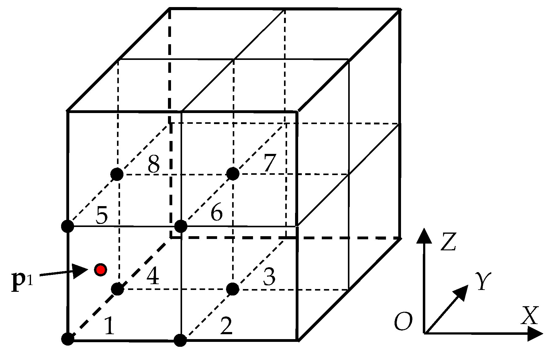
According to the previous hypothesis, the points in Q are nearly on the same tangent plane that is associated with projection points and the change of the normal vector is nearly linear in a small space. Using the projection points and their normal vectors, the normal vector for the point X_t = (x_t, y_t, z_t) can be calculated using a bi-linear interpolation.

The interpolation involves eight adjacent cubes as shown in Figure 2. For convenience, the cubes are indexed from 1 to 8. Because of the continuity of the unknown isosurfaces, if the cube contains point data and projection point, these points can be considered on the same tangent plane, and the interpolation can be transformed into two dimensions by projection. For convenience, we are projecting along the maximum component of the normal vector.

Let n₁ = (n_x1, n_y1, n_z1) is the normal vector of p₁, and |n_z1|≥|n_y1|≥|n_x1|, then the projection direction is the Z axis. Search the cube 1 and 5, 2 and 6, 3 and 7, 4 and 8 in Figure 2 to get the point p₁, p₂, p₃, p₄ with the normal vectors n₁, n₂, n₃, n₄, separately. Projecting all points in a cube (i, j, k) and p₁, p₂, p₃, p₄ along the Z axis, we get projection points in Figure 3. When the one of |n_x1| and |n_y1| is maximum, the process is the same with search order 1 and 2, 3 and 4, 5 and 6, 7 and 8, or 1 and 3, 2 and 4, 5 and 7, 6 and 8 to get p₁, p₂, p₃, p₄, and the projection direction should be X axis or Y axis.

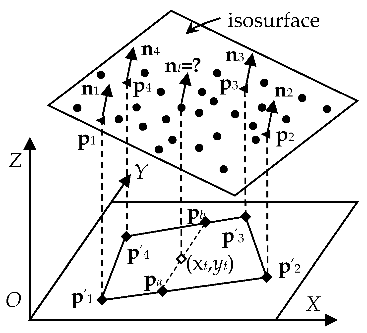
Suppose that the projection points p′₁ = (x₁, y₁), p′₂ = (x₂, y₂), p′₃ = (x₃, y₃), p′₄ = (x₄, y₄). The normal vector of point p_a = (x_t, y_a) and p_b = (x_t, y_b) in Figure 3 can be calculated by linear interpolation between the projection points of p′₁, p′₂ and p′₃, p′₄ separately. The y components of p_a and p_b can be obtained by linear interpolation:

$$\{\begin{array}{l}{y}_a=\frac{x_2-x_t}{x_2-x_1}{y}_1+\frac{x_t-x_1}{x_2-x_1}{y}_2\\ y_b=\frac{x_4-x_t}{x_4-x_3}{y}_3+\frac{x_t-x_3}{x_4-x_3}{y}_4\end{array},$$

(15)

In order to get the correct interpolation results. The direction of the normal vectors n₁, n₂, n₃, n₄ must be the same. If the dot product n₁·n₂ < 0, then replace n₂ with −n₂. After the normal vectors n₂, n₃, n₄ are consistent with n₁, the normal vector n_a can be calculated by interpolation between n₁ and n₂, and the normal vector n_b can be got by interpolation between n₃ and n₄:

$$\{\begin{array}{l}{n}_a=\frac{x_{e2}-x_t}{x_{e2}-x_{e1}}{n}_1+\frac{x_t-x_{e1}}{x_{e2}-x_{e1}}{n}_2\\ n_b=\frac{x_{e2}-x_t}{x_{e2}-x_{e1}}{n}_3+\frac{x_t-x_{e1}}{x_{e2}-x_{e1}}{n}_4\end{array},$$

(16)

Then, n_t can be calculated by linear interpolation between n_a and n_b:

$$n_t=\frac{y_b-y_t}{y_b-y_a}{n}_a+\frac{y_t-y_a}{y_b-y_a}{n}_b,$$

(17)

Without loss of generality, when the tangent plane is not intersected with the cube, the corresponding projection point can be set to p′_w = (0, 0), in which w = 1, 2, 3, 4.

3. Results

In this section, we tested the proposed methods and the existing methods with various synthetic and real point sets. When using SVD to compute the normal vector, the iteration will be stopped when the absolute error or the relative error reaches a value that is less than a given tolerance 1 × 10⁻⁶. Since the length of the cube has an important impact on the algorithm, unless otherwise specified, the length of the cube is 1.0L. In order to test the robustness of the proposed algorithm, we chose a set of typical point sets including free-form surfaces, planes, and other irregular point cloud models. Since the normal vector is very sensitive to light, we use the shading model to observe the small changes in the normal vector. All the experiments were run on a computer with Intel Core i5, 2.67 GHz CPU and 4 GB memory, running windows 7 (64 bit).

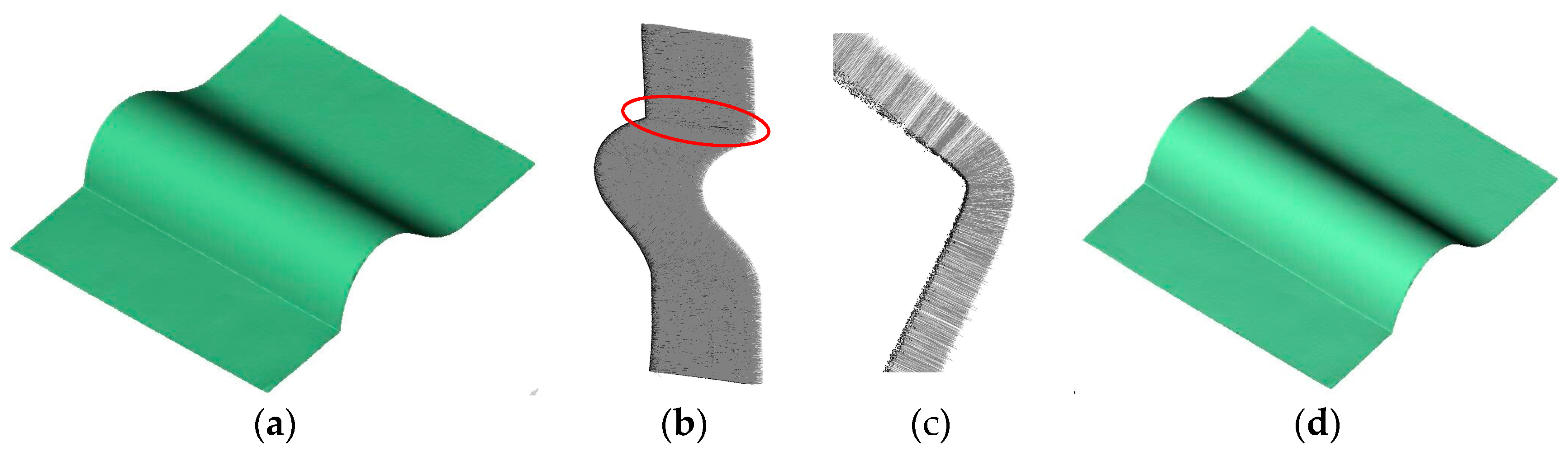
Figure 4 shows the normal vector result of a free-form surface model. The model contains 0.712 million points. Figure 4a is a shading model obtained using our method. In the calculation process, 376 × 314 × 93 cubes were constructed, of which only 134,832 cubes contained points data (about 1.23%). It takes 1014 ms to estimate the normal vector, including 202 ms for the normal vector interpolation and 812 ms for the nearest neighbor search and the PCA algorithm. Figure 4b is the normal vector that is attached to the point cloud. Figure 4c is an enlarged image that shows that the method performs well when dealing with sharp changes of surface. Figure 4d is the shading model obtained by the ENN based algorithm, and it takes 3762 ms to estimate the normal vector, which is about 3.7 times more than our method. This is mainly due to the fact that our algorithm avoids more than 80% of the matrix decomposition.

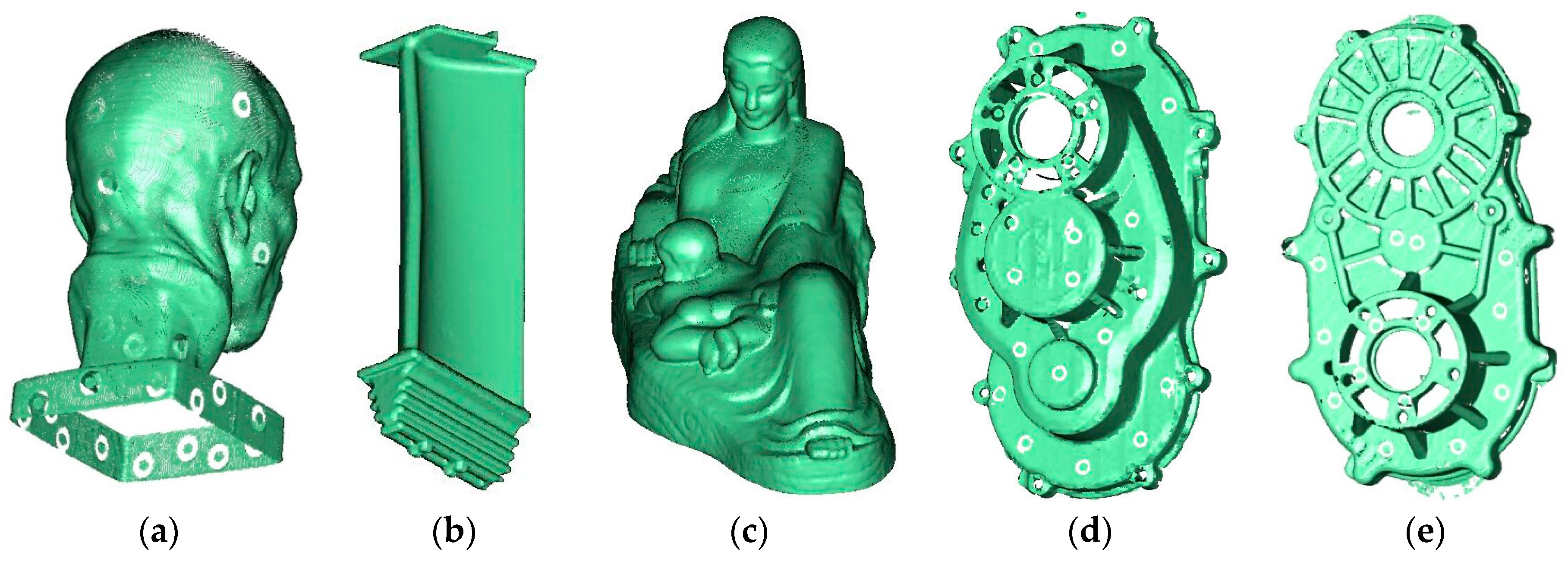
Figure 5 shows the results on several point sets with different numbers and complexity. The point cloud contains 0.121, 0.178, 0.516, 1.272, and 2.875 million points, respectively. The proposed method can deal with not only smooth transition surfaces but also the models with complex shapes and shape changes.

To be objective, we estimate the normal vector for these points clouds using the EGG-based method presented by Park [6]; the ‘k’ value is set to 8.

Table 1. The details of the experiment.

Object Model	Points (million)	Projection (million)	Cubes	Time (ms)	Time (3.0L) (ms)	Time of EGG (ms)
Famer Statue	0.121	0.038	156 × 102 × 121	234	101	924
Blade	0.178	0.078	101 × 143 × 383	266	139	1253
Mother Statue	0.516	0.114	297 × 200 × 134	828	353	2742
Engine Cover	1.272	0.248	444 × 267 × 162	2259	846	6759
Engine	2.875	0.450	621 × 314 × 191	5023	1802	16,130

is the details of point number, projection point number, the cubes constructed by our method, and the comparison of the normal vector estimation with the EGG-based algorithm. The number of points and projection points in Table 1 is counted in the millions, and the unit of the time in Table 1 is millisecond. With the increase of the point cloud number, the time of algorithm increases, but the time of the nearest neighbor search and normal vector estimation is obviously slower than the normal vector interpolation.

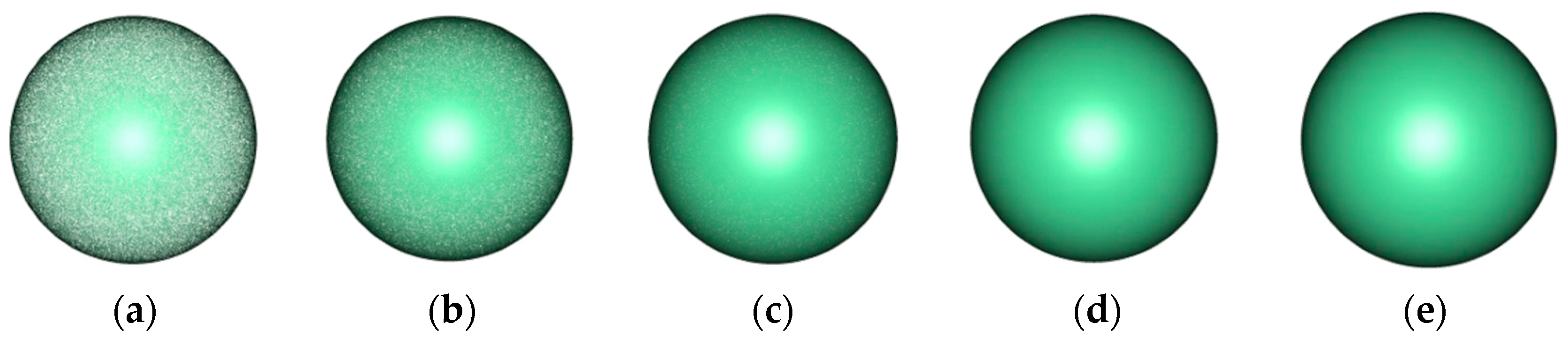
We carried out experiments on the simulation of spherical point cloud data; the results are shown in Figure 6. From (a) to (e), the number of points in the simulated spherical point cloud is 0.1875, 0.375, 0.75, 1.5, and 3.0 million points, respectively.

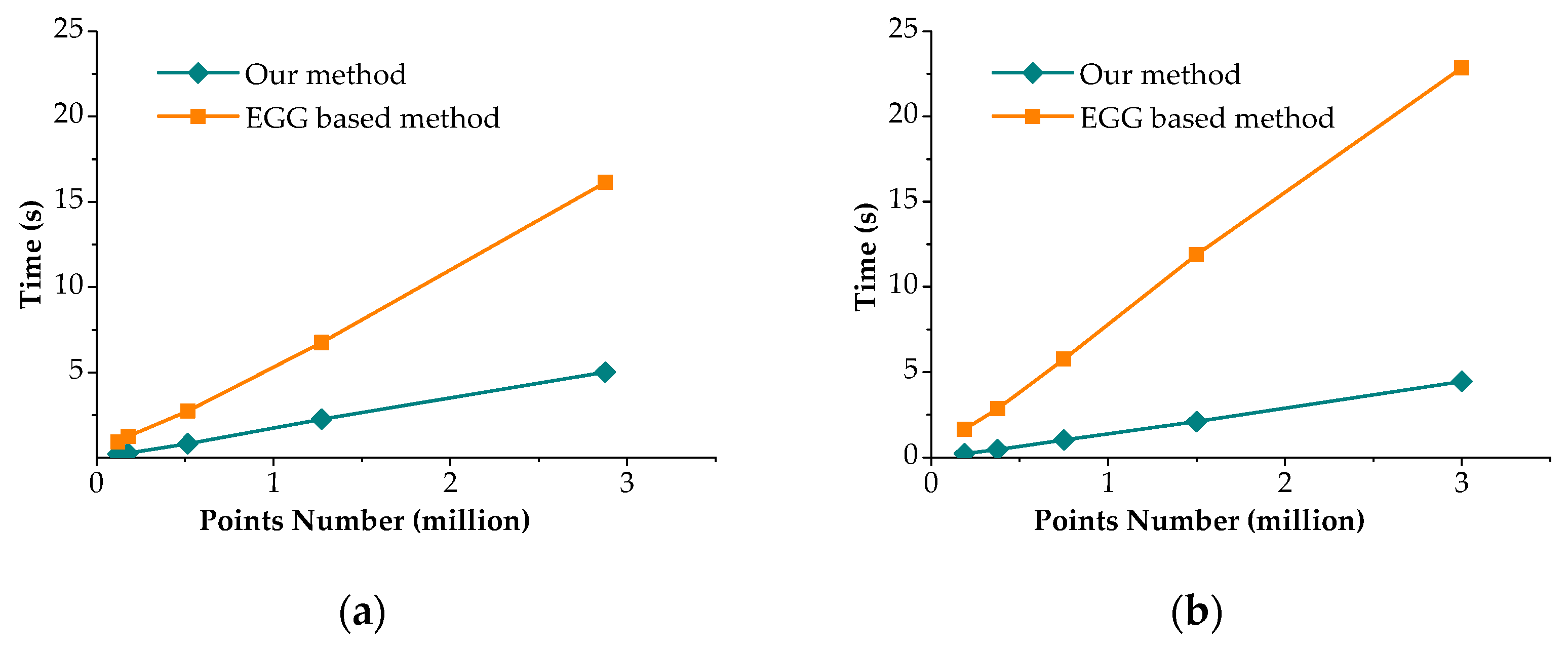
We tested the proposed algorithm and the EGG-based algorithm on the actual data and the simulated data, and plot the results in Figure 7a,b. The efficiency of the two algorithms is consistent with the data in Table 1. The average number of neighborhood points in our algorithm can reach 15, and Figure 7 shows the result that our algorithm is 3–4 times faster than the latter, and this is due to the fact that our algorithm requires less nearest neighbor searching and SVD operations. Once the length of cube’s edge L is determined, the projection points are determined, and the projection points are usually far less than 1/3 of the number of the points. Our algorithm consists of the following steps: create hash table, search hash table, Create 3D points, compute normal vector, and interpolation. The computation complexity are O(N), O(1), O(N), O(N), and O(N), respectively. The time complexity of our algorithm is O(N). We can get the same conclusion from Figure 7.

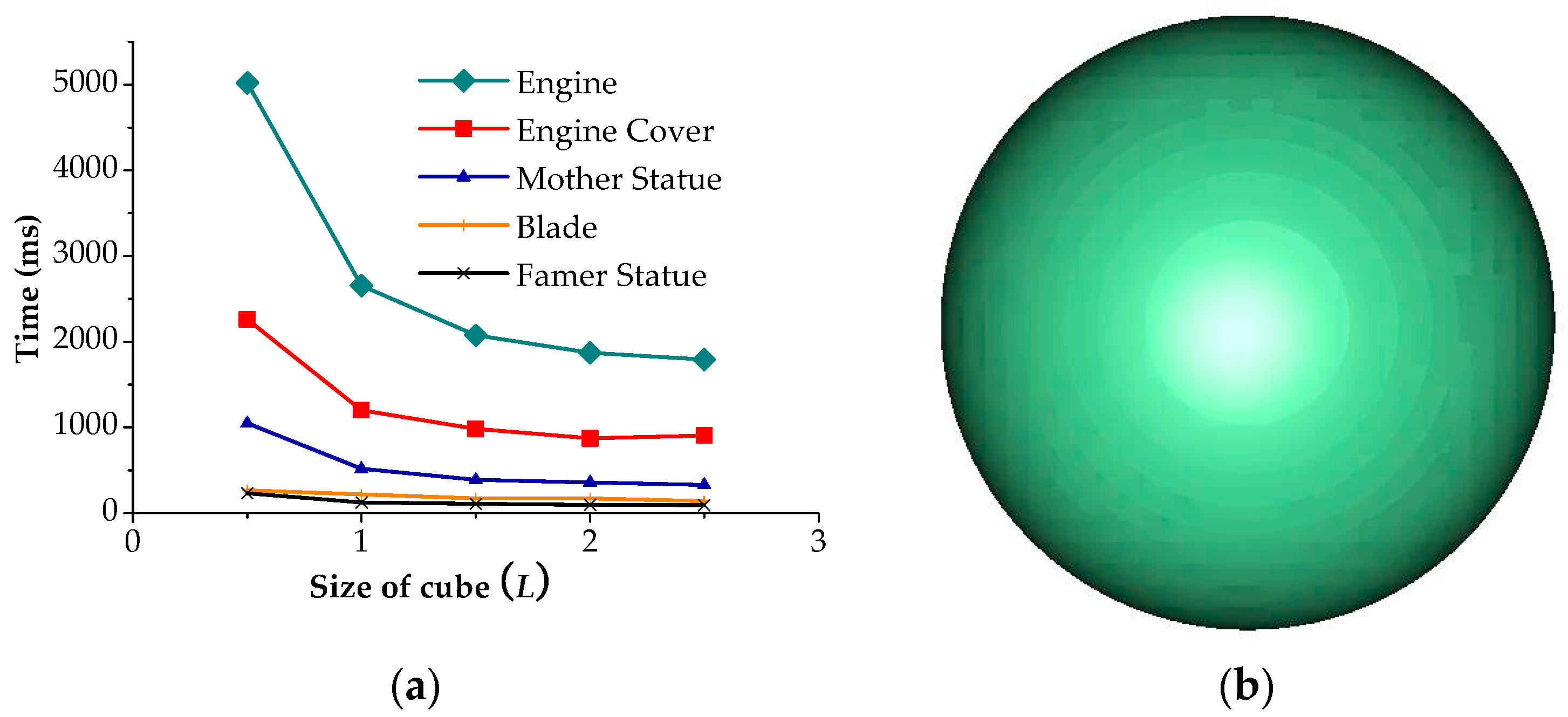
The number of projection points is the key factor in determining the efficiency of the algorithm, which is closely related to the length of the cube. We have tested the length of the cube, which varyies from 1.0L to 3.0L on the model in Figure 5, and gotten time-length curve. The curves about time and L are nonlinear, and the ordinate decreases sharply with the increase of L. Figure 8a shows the result of the normal vector estimation of different lengths of the cube. When the cube’s length is over 2.0L, the time remains almost the same. The reasonable length of cube is about 1.5L, which ensures the efficiency and accuracy of the algorithm. Figure 8b is the result of the normal vector estimation of simulation spheres, and the error greatly increased, while the length of the cube is over 3.0L.

We have explored the proposed algorithm on simulation sphere data in terms of accuracy, and the statistical results show that the average deviation of the normal vector is less than 0.0065 mm. In our algorithm, over 75% interpolation calculation uses four normal vectors with an average error of 0.005 mm,;14% interpolation calculation uses three normal vectors with the average error of 0.008 mm; and 11% interpolation calculation uses two normal vectors with the average error of 0.0102 mm.

The experimental results show that the proposed algorithm is more effective and efficient compared with the existing methods of the normal vector estimation.

4. Conclusions

A new bi-linear interpolation based method for estimating the normal vector for LSSPC has been presented in this paper. The point cloud is segmented by many small cubes according to the Marching Cube algorithm, followed by a neighborhood search for the projection points of the isosurface and the cubes. The normal vector estimation for the projection points was realized by the principal component analysis algorithm using these neighbor points. In order to calculate the normal vector of the point cloud, the bi-linear interpolation was carried out through 4 adjacent normal vectors of the projection points. Experimental results on several practical and simulated point clouds demonstrated the efficiency and the accuracy of the proposed method.

The most critical step of the algorithm is to calculate the normal vector by the bilinear interpolation. The condition of realizing this calculation is to project the point along the direction of the normal vector approximately, so that the three dimensional problem is transformed into a two dimensional problem. The new normal vector estimation algorithm has helped our research on data rendering, feature recognition, and data analysis for 3D point cloud with the efficiency of calculation greatly improved.