1. Introduction
All sectors of the economy need energy services to meet basic human needs (lighting, cooking, comfort, mobility, communications, etc.) and to support production processes. Since about 1850, the global exploitation of fossil fuels (coal, oil and gas) has increased to provide the bulk of energy supplies, resulting in a rapid increase in greenhouse gases emissions (GHGs). Access to energy is fundamental to the development of societies. However, most of the energy used in the world comes from fossil fuels whose reserves have been decreasing. However, energy consumption increases and with it all associated economic, social and environmental impacts [
1,
2,
3].
Climate change is caused by changes in the atmosphere that result from its chemical transformation by GHGs. This disturbance of the atmospheric equilibrium is expressed by an increase in average temperatures on Earth, modifying its physical, chemical and biological characteristics. The impacts on the environment are multiple, important and increasingly frequent: droughts, melting glaciers and sea ice, rising sea levels, and tropical storms. They affect the entire world population and global biodiversity. Human activities are the main contributors to current climate change and its impacts on the environment. Indeed, according to the Intergovernmental Panel on Climate Change (IPCC), global warming is very real and human activity is responsible for it, through the emission of GHGs [
4].
Reducing GHGs emissions is essential. In the residential sector, the quality of the buildings and their associated comfort has increased particularly in recent years. Hygiene needs, basic needs in food preparation and preservation, the need for thermal comfort (heating and cooling), and the use of entertainment equipment and electrical equipment to support tasks (personal computers, household appliances, etc.), are facilities that were gradually being made available to the users of residential buildings. However, this higher level of comfort usually translates into increased investment and increased energy consumption [
5] with a consequent increase in the emission of gases that contribute to global warming. To achieve this, we need to change our behaviors and ways of life. We will also have to adapt to new climatic conditions. The two strategies go hand in hand because the adaptation effort will be less if we do more to limit the magnitude of climate change. Besides, the residential sector has a great potential for GHG emissions reduction with plenty of room for improvement [
6]. Currently, rational energy consumption is one of the most debated issues within the context of sustainability, since most of the energy consumed comes from non-renewable sources. Sustainable consumption is a set of practices related to the acquisition of products and services that aim to reduce or even eliminate impacts to the environment [
7].
Our society seeks a constant improvement in the quality of life and, therefore, increasingly demands sustainable buildings [
8]. Despite this, the attention given to the waste of energy in buildings is still low, both at the construction level (for example, the adequacy of the buildings to the climate in which they are), and the rational use of the energy inside [
9].
Energy consumption in the domestic sector depends directly on households’ disposable income. The sustained growth of this indicator, which has a strong impact on the possession and use of energy-consuming appliances, has been one of the drivers of the demand for electric power in the sector. Another reason for the increase in energy consumption lies in the enormous multiplicity of small and large inefficiencies resulting from both the consumer equipment used in the sector itself, buildings included and the procedures and usage habits of such equipment. It should be kept in mind that residential buildings are used by many millions of consumers, and there is some inertia in the adoption of efficient energy consumption standards, due not only to consumer behavioral reasons but also to the period necessary for the replacement of equipment and progressive restoration of buildings [
10].
The housing and services sector, composed mostly of buildings, absorbs circa 40% of final energy consumption in the European Union and 39% in the United States, and is in the expansion phase, a trend that is expected to increase energy consumption [
1]. The energy necessary for the operation of a building is mainly used to maintain thermal comfort and also in the use of electrical equipment that covers other functions than AC, such as lighting, computer equipment, elevators, etc. The amount of energy used in the AC depends on the overall insulation level of the thermal envelope (sufficient thickness of the insulation, reduction of thermal bridges and tightness of the joinery) and the degree of efficiency of the thermal installations [
11].
The amount of energy necessary to have a good thermal comfort in a building depends not only on its volume, orientation, rigor of the climate and temperature to be maintained, but also on the heat losses or gains that the building has through its external envelope, which determine the energy demand of the building for AC. The degree of thermal insulation of the external enclosures of the building and its tightness are determining factors of these heat losses or gains, as well as the proportion of the façade surface in relation to the volume of the building [
12].
Intelligent sector coupling will address new approaches to the use of efficient and renewable energy systems in residential and commercial areas. Considering the background of a building control system, which includes an energy-optimized system and data management, the interplay of electricity, heat and mobility needs to be rethought. Therefore, the elements of the building to be considered for saving and energy efficiency are: the insulation and the sealing of the building, the thermal installations, the electrical installation, AC, the lighting and the equipment for the treatment of the information and facilities for the use of solar thermal and photovoltaic energy [
13].
The concept of building energy management systems caught the attention of researchers for quite some time [
14]. Energy management is not a new application of home automation and building automation systems have begun to introduce the control of energy demand in the home using a home automation system. Typically, these systems target commercial office buildings to manage the consumption of heating, AC, domestic hot water and lighting services. Today, this management system ensures the control and operation of the “Smart Home” for better energy performance of facilities, and better comfort, such as heating control [
15].
A home automation system consists essentially of household appliances connected via a communication network allowing interactions for a management purpose. Via this network, we can turn an ordinary house into a smart home. As a result, the building is a complex living space where production and energy consumption systems vary widely from one space to another but also where the occupants express demands for complex services. Indeed, the energy manager will be able to control the different automation of the building (start of the washing machine, reference temperature and on/off for heating, opening or closing flaps, lighting, ...) [
16].
In a building the AC system is responsible for approximately 40% of electric energy consumption. If involving heating, cooling and air movement activities it could be 45% of total power consumption of a building [
17] and as high as 60% in countries such as Canada. The increase of electric energy has motivated the development of new technologies to reduce consumption [
18]. Thus, AC systems have to be operated as much energy efficiency as possible.
In this sense, several benefits can be enjoyed by implementing energy and cost saving actions into the controller design of the AC unit. To achieve these gains in savings, an improvement could be made in the AC control systems by implementing superior controllers which in turn can improve and optimize the consumed energy and consequently the cost. On top of a superior controller design, such type of measure is cost effective for the existing households and their AC systems. Fortuitously, a new controller for the AC unit costs far less than a new edifice or the installation of a new mechanical system. The majority of the installed AC units utilize the elementary ON/OFF controllers based on a thermostat. In the absence of a complex controller could culminate in both operation and cost disadvantages such as more energy consumption, greater cost, thermal discomfort and accelerated equipment deterioration [
19]. Thus, the room for improvement for AC units is wide by implementing a more advanced controller [
18].
Motivated by the current developments in the area of big data, in the field of communication, and increasing processing power of the microcontroller units (MCUs), a more advance control method is presently conceivable to be implemented in AC units in order to overcome the abovementioned shortcomings in AC control. A promising opportunity in this regard with the potential to achieve greater energy saving results in AC units is the employment of home energy management system (HEMS) control methods. Such types of energy savings typically relies on the ideal operation scheme employed in HEMS, capable of decreasing the consumption of energy and at the same time capable of decreasing the thermal discomfort [
20]. This kind of energy controllers happen to be a trustworthy enhancement for households and are easily ran, installed or substituted. Therefore, with the purpose of increasing the energy savings in a room, is of great importance for the automation of optimization operations to emphatically adjust the AC unit operation mode to the indoor and outdoor conditions [
21].
A key advantage of smart controllers is the capacity to perform more efficiently and the capacity of demand-side management (DSM) [
22]. For consumers, such an option could mean cost reductions on the energy bill, especially in regions where ToU tariffs are already enforced. Thus, the deviation of the load lets the consumer to reap the benefits in running the appliances during periods with lower prices [
23]. Therefore, the concept of DR has a strong potential for helping consumers to decrease their electricity bill by reducing the energy consumption during peak periods and is essential for the optimal operation of HEMS [
24]. The implementation of an effective DR process is a vital element during the design of HEMS [
25]. For this reason the study of this concept has drawn a lot of attention from the research community [
26].
The Model Predictive Control (MPC) refers to a class of computational control algorithms that use an explicit model to predict the behavior of future plant outputs. This technology is widely used in the chemical process industry and is generally the standard technique used in advanced control applications. The MPC emerged in the late 1970s, when Cutler and Ramaker (1979) proposed the so-called DMC (Dynamic Matrix Control) [
27]. Since then, several articles have been published and this area has achieved great development. In [
28] can be found a review of MPC theory and applications to HVAC systems and other modeling techniques used in building HVAC control systems can be found in [
29]. The philosophy of the predictive control (MPC for Model Predictive Control) comes down to “using the model to predict the behaviour of the system and choose the best decision in the sense of a certain cost while respecting the constraints”. A linear model is generally used in numerous industrial cases, thus the application of the MPC is justified in such occasions. This is partly due to the simplicity of designing linear models which translates into less computational efforts [
30].
Many researchers have addressed the issue of controlling the air conditioning home systems through different control methods along the years [
29,
31]. A more generalized approach for mixed-integer predictive control of HVAC systems using (mixed integer linear programming) MILP is presented in [
32]. To improve the wind power utilization level in the distribution network and minimize the total system operation costs, Wang et al. in [
33] propose a MILP based approach to schedule the interruptible air-conditioning loads. In [
18], Afram et al. implement and validate a model predictive control (MPC) based supervisory controller which is designed to shift the heating and cooling load of a house in Toronto to off-peak hours. A hierarchical decomposition for economic MPC in large-scale commercial HVAC systems using a two-layer approach is proposed in [
34]. A case study in which artificial neural network (ANN) models of a residential house located in Ontario, Canada are developed and calibrated with the data measured from the location is addressed in [
19]. In [
35], Parisio et al. present an experimental case study of a scenario-based MPC for HVAC systems. In [
36] an experimental implementation of whole building MPC with zone based thermal comfort adjustments is presented. A prototype embedded system is developed in [
37] to emulate an adaptive environmental control strategy algorithm to numerically determine an indoor comfort temperature for a real-time control in an air-conditioning system. A demand side response modeling with controller design using aggregate air conditioning loads and particle swarm optimization is presented in [
38]. In [
39], Smith et al. present a DR strategy to address residential air-conditioning peak load in Australia. An automatic AC control with real-time occupancy recognition and simulation-guided model predictive control by using Raspberry Pi 3 is presented in [
40]. In [
41], Ascione et al. present a mono-objective genetic algorithm (GA) that minimizes global costs for space conditioning for cost-optimal building design integrated with the multi-objective model predictive control. In [
42], the problem of scheduling deferrable appliances and energy resources of a smart home is addressed considering a variety of sources applying a multi-time scale stochastic MPC. In addition, in [
43], distributed energy resources scheduling problem of the set of smart homes (SHs) has been investigated considering their cooperation with their neighbors by applying a stochastic MPC. In [
44], the implementation of demand response (DR) programs is investigated considering the nonlinear behavioral models of the residential customers.
It is proposed in this paper to compare three control options for an AC unit, ON/OFF, PID and MPC. However, instead of adopting a linear power switch, a two level control signal interface for the MPC that modulates the bounded continuous set of manipulated variables to a discrete set of integers is used in this paper, as described in [
45]. This AC unit controls the temperature of a room governed by six distinct DR electricity ToU rates. One ToU rate is an hourly price signal during 24 h while the remaining five ToU rates are the presently existing ones enforced by the Portuguese electricity retailer [
46]. In the case of this model, the home is equipped with a PV solar panel. The selected setting for this study was the Portuguese city of Évora because it is a pilot city in a DR project—InovGrid [
47]. In the model for this paper, an entire week of summer—July 2016—was investigated. The reason for picking this week is that the records confirm a noticeably high ambient temperature and a high solar irradiation. The overall purpose is to compare the overall weekly expense of each studied tariff option for every control method and in the end to reach an optimal solution.
The rest of the paper is structured as follows. In
Section 2, an overview of the MPC control method can be observed. In
Section 3, the model of the room is thoroughly described. A detailed result analysis and discussion can be found in
Section 4. The overall conclusions are stated in
Section 5.
2. Model Predictive Control
With the increasing complexity of industrial plants and the search for better systems performance, the development of new controllers is increasingly important. Among the advanced control techniques suitable for industrial applications is model predictive control (MPC) [
48,
49,
50,
51].
The concept of prediction is increasingly used in several sectors beyond the control of processes themselves: maintenance, cost forecasting, early detection of malfunctions, etc. This concept has been increasingly complementary to feedback, the action is more related to reaction than to anticipation or prediction. The feed-forward control is naturally encompassed by the concept of prediction. The basic idea of predictive control is simple: based on a model of the process, the behavior of the process is predicted for different actions (controls) [
52]. From the optimization of a functional, dependent on these actions, the optimal action to be applied to the process is obtained [
53].
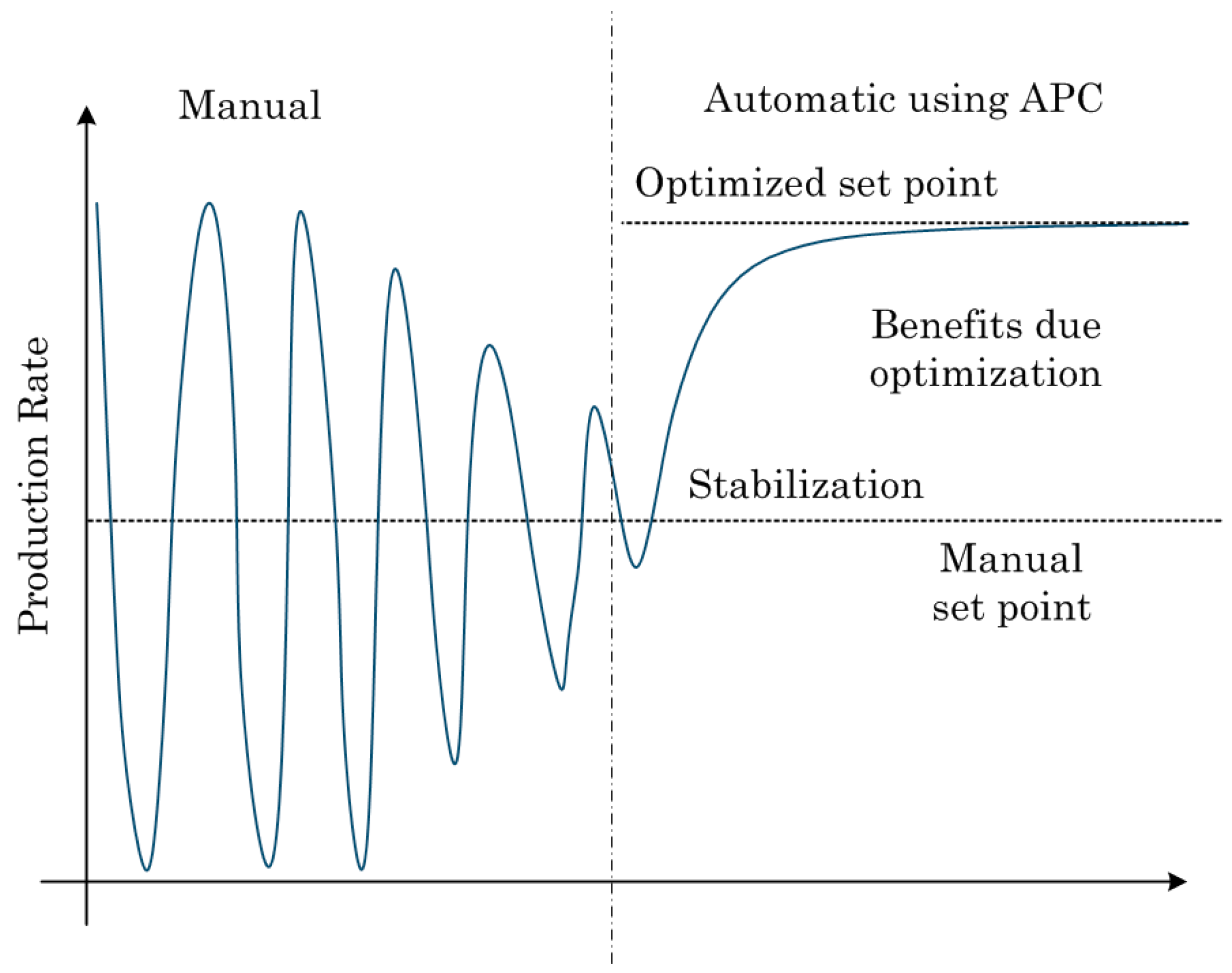
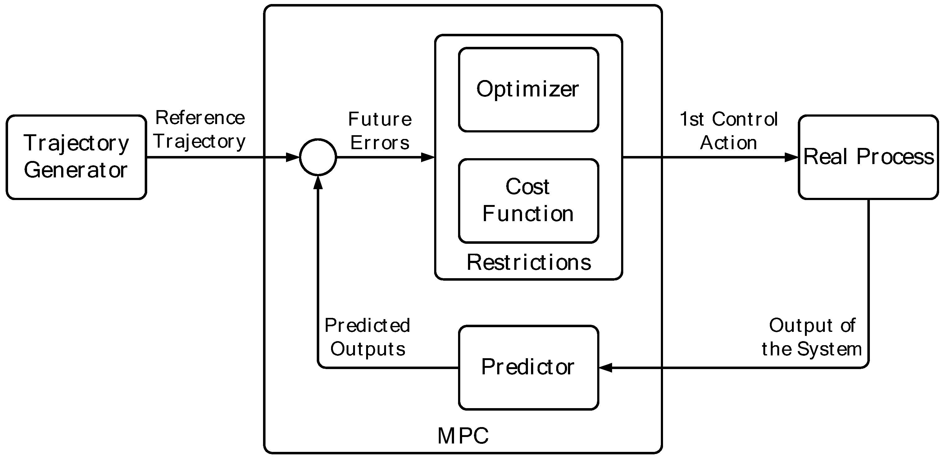
MPC is not a specific control strategy, but is the name given to a set of control methods that were developed considering the concept of prediction and obtaining the control signal, by minimizing a certain objective function [
54]. It is advanced process control (APC) with less variation in process variables [
55]. This function considers future error and constraints on process and/or control variables [
56]. An overall operation of this control method can be observed in
Figure 1.
A major advantage of linear MPC compared to non-linear is the associated optimization problem and simpler to solve. However, when processes have a medium or severe degree of non-linearity, when there is a range of operations and variables, or when the processes undergo continuous transitions in their operation, a nonlinear model of control design must be considered, so that it allows maintaining stability and the desired performance for the closed loop system [
57].
The MPC rather than a specific controller is a methodology for the calculation of control actions. It is also a comprehensible methodology, which in a way tries to reproduce the way an expert operator would operate in the control of a certain process [
48].
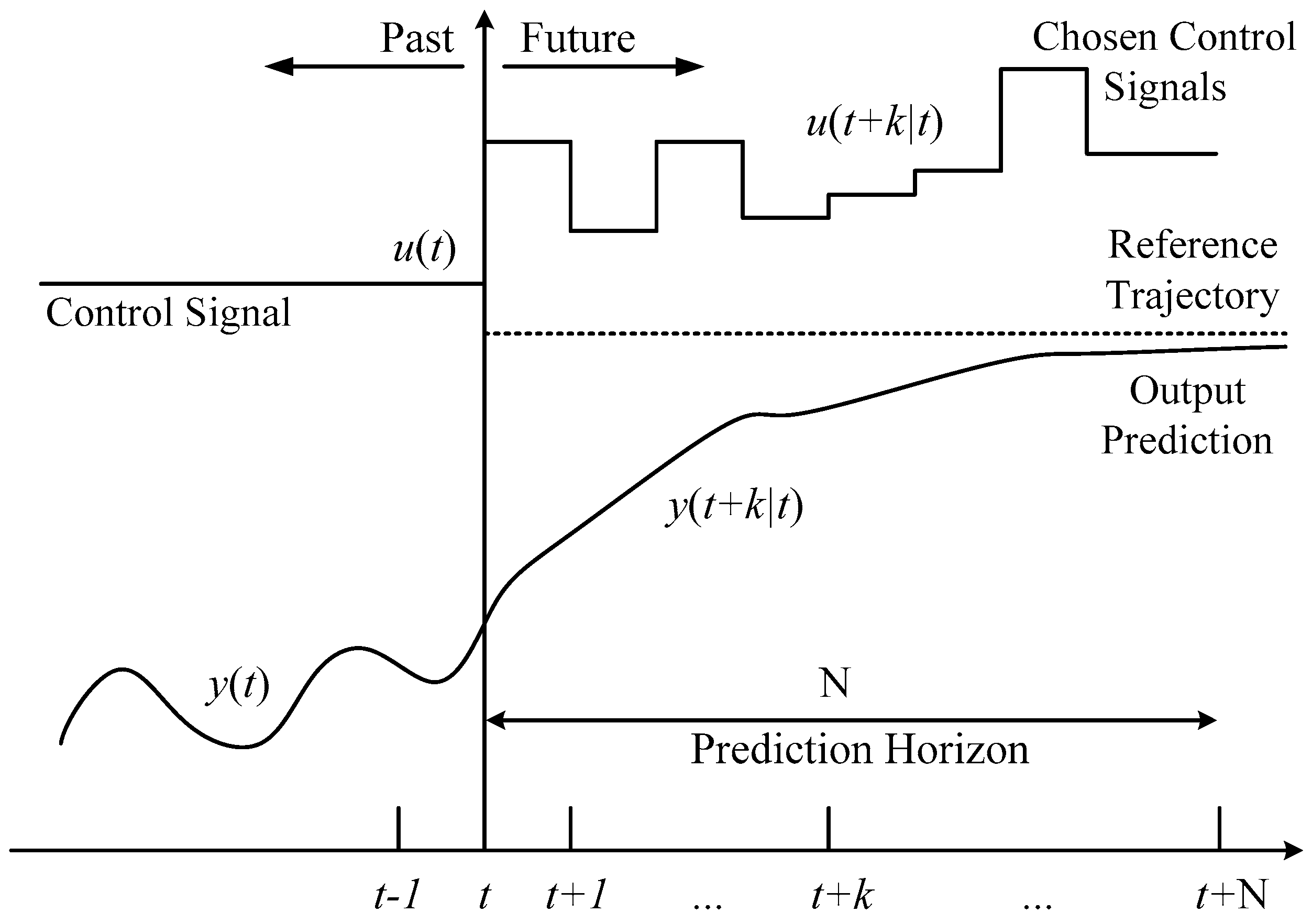
To achieve a higher quality control, this same operator would repeat all the calculations whenever it has updated information, being new measures of the status of the process or updated knowledge about the behavior of the process (new information of the model). In the MPC, this concept is called the receding horizon, resulting in the resolution of a different optimization (minimization) problem in each sampling period, since new information is incorporated in the dynamic evolution of the process [
55]. The concept of a receding horizon can be seen in
Figure 2.
This example allows understanding that the first controls performed manually by operators who knew the process well could have been included in the area of model-based predictive control. In short, it is a very intuitive methodology to address the control of a process and this has influenced its dissemination at an industrial level [
58].
Based on the process model, the predictor is responsible for calculating, for each instant
t, the predictions of the dynamic evolution of the process [
y(
t + 1|
t), ..., and
y(
t +
N|
t)]
2 throughout the horizon of prediction
N, from the dynamic information available up to that moment (measurements of the process variables and inputs passed up to the current time
t) and a postulated or future control law [
u(
t|
t), ...,
u(
t +
N|
t)], along the prediction horizon, as shown in
Figure 3 [
48].
Future control actions are calculated in a way that minimizes a certain cost function. Thus, the cost function assigns a value to each prediction and therefore to each postulated control law. This value tries to show the degree of compliance with the static and dynamic specifications compatible with possible operating restrictions. Therefore, the main objective of the cost function is to keep the output of the process and (
t +
k|
t) as close as possible to a reference trajectory
w (
t +
k) that describes how you want to guide the output from your current value and (
t) up to your future points of consignment. The cost function thus generally takes the form of a quadratic function of the errors between the predicted output and the reference trajectory. In addition, in most cases, it usually includes some term referring to the control effort [
56].
In the case of the optimizer, the vector of control actions that offers the best value of the cost function must be found. Generally, in this search process, the optimizer performs postulates of the control law and iteratively tries to approach the optimal control law. In addition, if the cost function that is defined is quadratic, the model used is linear and there are no restrictions for any signal involved, then it is possible to find an analytical solution for the optimization problem. Otherwise, it is necessary to use, in general, a numerical optimization method.
Once the sequence of future control actions is calculated, which at that moment makes the cost function optimal, the concept called receding horizon is used [
59]. Only the first of them is applied as input to the process
u(
t|
t), neglecting the rest, since at the next instant
t + 1, the output
y (
t + 1) is already known, and with that new information the points are repeated 1, 2 and 3, obtaining in this way the control signal
u(
t + 1|
t + 1) to apply at that moment (which is not equal to the one that had been postulated at the previous instant
u(
t + 1|
t)).
The analysis of this control methodology shows that, whatever the implementation is, any predictive control based on models can be understood as an optimization problem in each sampling period (mobile horizon) that consists of three fundamental elements: predictor, cost function and optimizer.
Combining different variations of these three fundamental elements can obtain many controllers that would be part of the family of predictive controllers. Thus, this diversity can be inferred, considering that different controllers will appear, depending on the type of model of the process used, according to the type of cost function used and according to the applied optimization method. To be able to propose any type of improvement, one must go through a first step of analyzing these three fundamental elements.
Almost all possible ways of modeling a process appear in some MPC formulations, the most used being the following: finite impulse response, step response and state space model.
The finite impulse response is also known by weighting sequence or convolution model. The output is related to the input by the equation:
where
hi are the sampled values obtained by subjecting the process to an impulse unit of amplitude equal to the sampling period. This sum is truncated and only
N values are considered (therefore, it only allows representing stable processes and without integrators), having:
where:
A disadvantage of this method is the many parameters you need, since
N is usually a high value (in the order of 40–50). The prediction will be given by:
This method is widely accepted in industrial practice because it is very intuitive and does not require prior information about the process, with which the identification procedure is simplified, while easily describing complex dynamics such as non-minimal phase or delays.
The step response is very similar to the previous one only now that the input signal is a step. For stable systems, you have the truncated response that will be:
where
gi are the sampled values before the step input
y:
The value of
y0 can be taken as 0 without loss of generality, with which the predictor will be:
This method shows the same advantages and shortcomings of the previous one.
The state space equations have the following representation:
where
x is the state and
A,
B and
C are the system matrices, input and output, respectively. For this model, the prediction is given by:
This method has the advantage that it also serves for multivariable systems while allowing to analyze the internal structure of the process (although sometimes the states obtained when discretizing have no physical meaning) [
60]. The calculations can be complicated, with the additional need to include an observer if the states are not accessible.
3. The Model of the Room
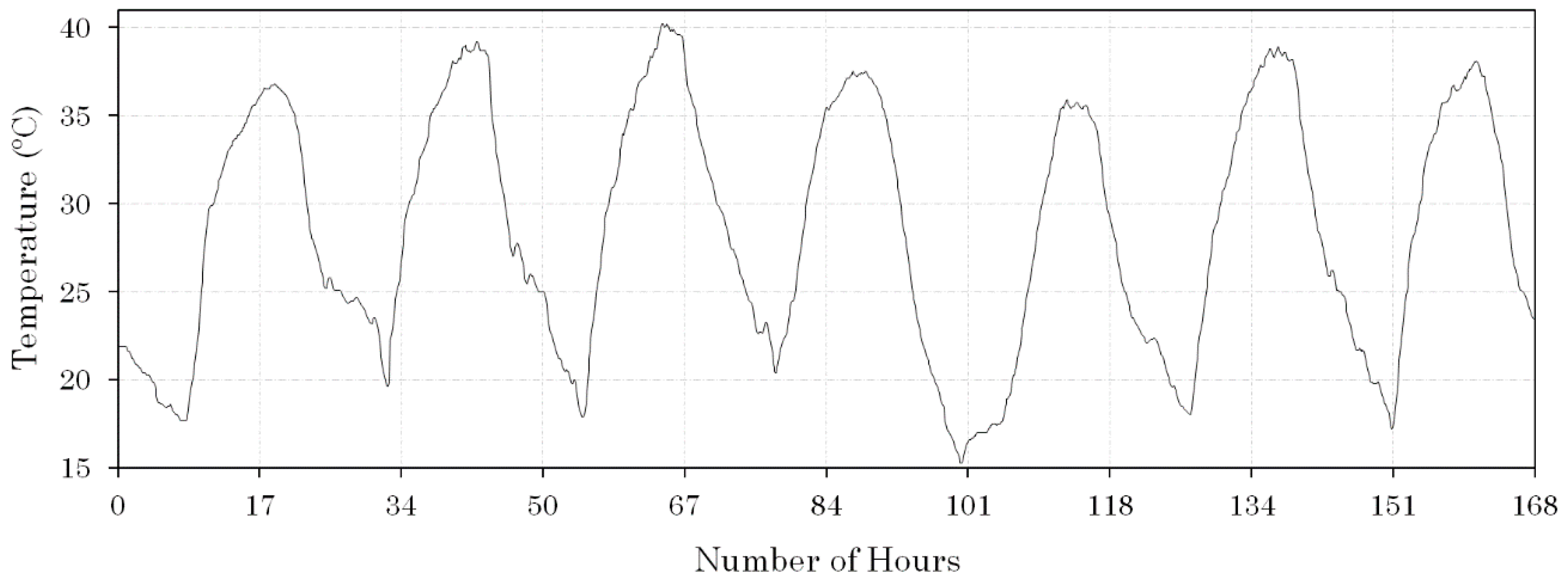
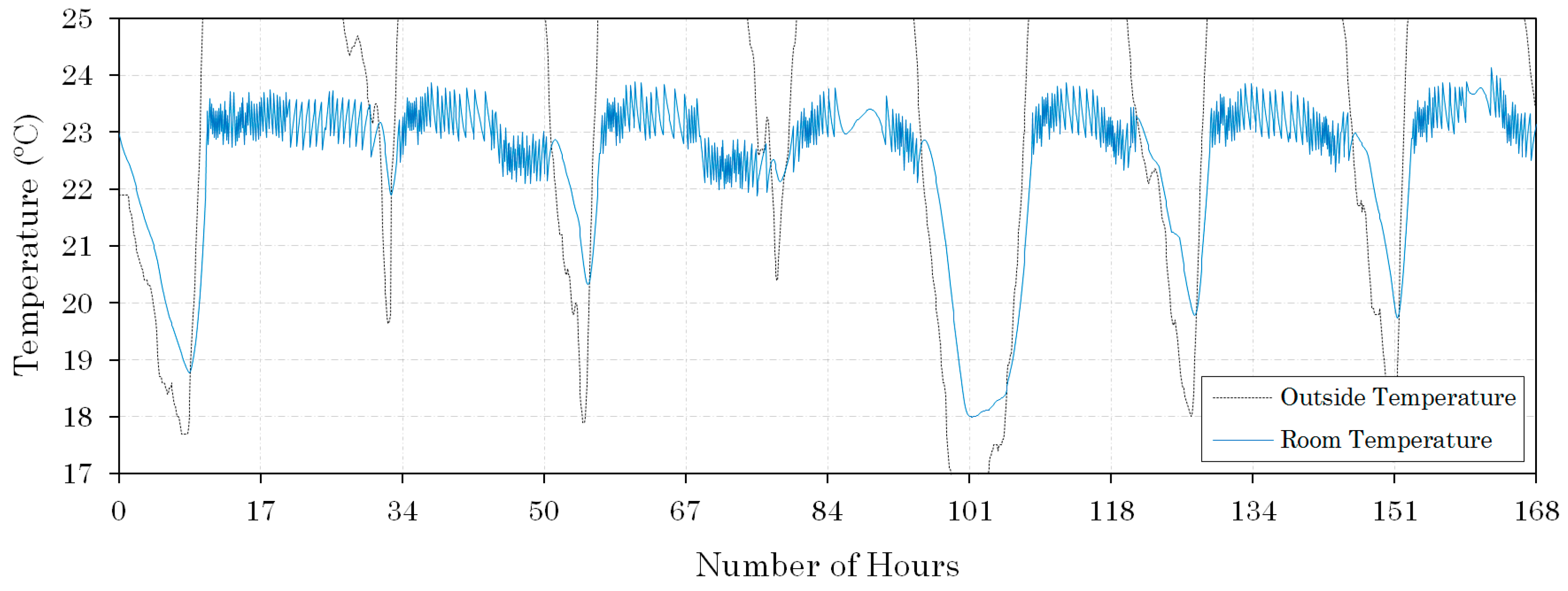
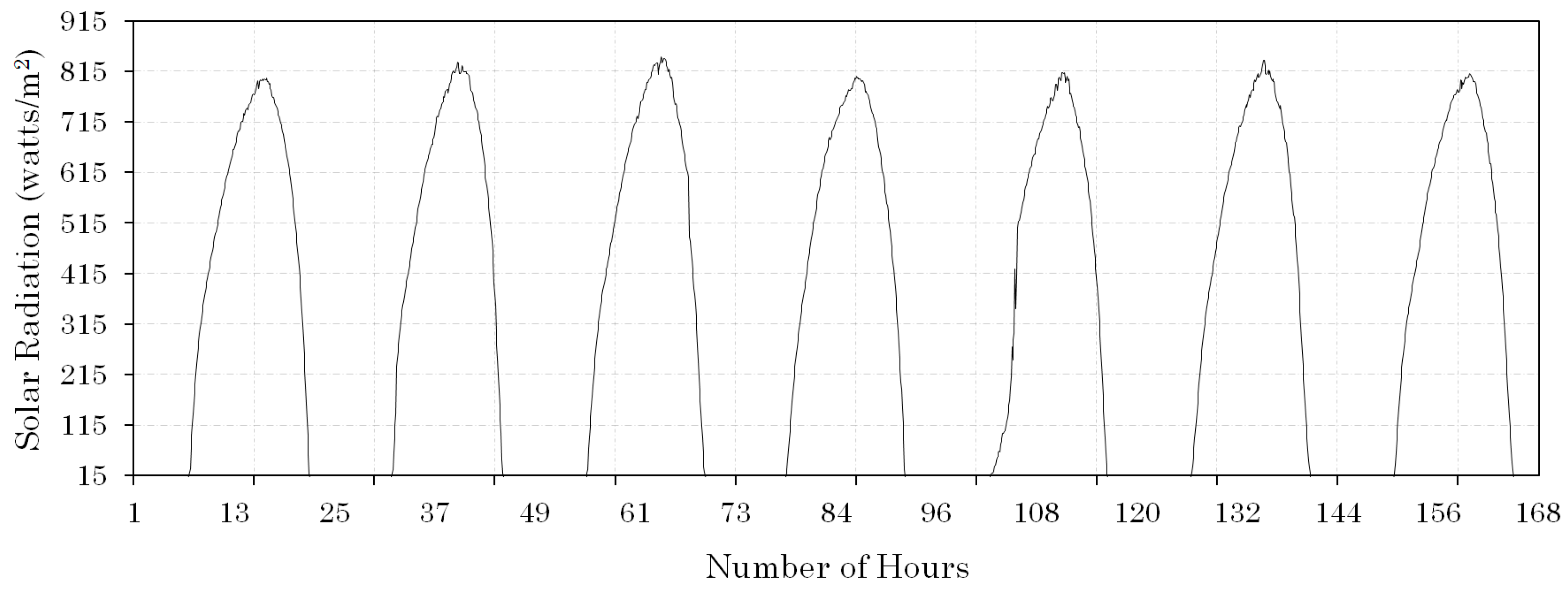
The room in this model is assumed to be cooled with an AC unit displaying a cooling capacity of 3516 kW. The exchange of heat with the outside air happens throughout the external wall of the room and through the window. This heat exchange is deemed the most important cause of disturbance of the picked thermal level of comfort. By taking into the account the purpose of this study, which is to test all three control strategies, the amount of the heat generation/loss through the outer wall of the room is modeled for an entire week (168 h). However, for this model, the week is separated by days. All three studied control methods have as reference 23 °C and the tolerance is ±1 °C. This temperature was chosen as such since it is a common selection for the AC in the studied region. In addition, for the sake of simplicity, it was assumed that the AC system works on a constant power. To take full advantage of the entire AC unit capacity, the chosen studied week is in the summer, typically with very high temperatures for this time of the year. The ambient temperature of the chosen week for the city of Évora for this period is shown in
Figure 4. The local solar irradiation for the same week can be observed in
Figure 5. Both ambient temperature and solar irradiation are the input data of the model. For the simulations of this model, a time step of 1 s is used in this study.
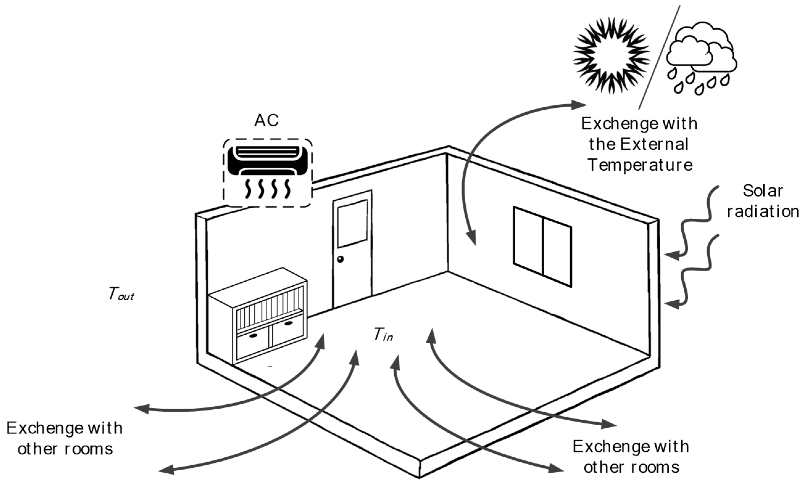
An additional portion of energy is required to be consumed if heat was to be inserted or removed for generating an enjoyable level of comfort regarding the temperature of the room. Therefore, the ideal level of comfort for the consumer is fixed by selecting the reference temperature and by measuring the indoor temperature. However, some elements could disturb this selected level, such as the thermal mass of the room and the exchange of heat through the outer wall of the room as depicted in
Figure 6. Consequently, the dynamics of the indoor temperature originates from such elements as the energy balance of the external temperature and the AC unit that insets or removes heat from the room in a constant readjustment with the thermal mass of the room which could also be seen in
Figure 6.
A resistance–capacitance circuit analogy of a thermal mass model is utilized in this study with the purpose to assess and compare the behavior of the controller. The studied model comprises the heat flow balance, the thermal capacitance of the indoor air and the external wall and room’s windows [
45]. The values of the physical parameters were taken from a previous study [
61]. One of the objectives is to ensure a uniformed temperature in the room and, due to this goal, it is implicit that the indoor air is mixed homogeneously. The mathematical description of this model is as follows [
62]:
In this model,
Qac embodies the cooling power input to the room,
Tout is the variable that represents the ambient temperature, the temperature of the room is given by
Tin,
Twl symbolizes the wall temperature and
Cwl symbolizes the thermal capacitance of the wall. The thermal resistance of the wall is given by
Rwl, the thermal resistance of the windows is characterized by
Rwd,
Cin represents the thermal capacitance of the interior air and
Qs gives the heat flow into an exterior surface of the room exposed to the solar radiation. In this model,
ho represents the combined radiation and convection heat transfer coefficient, and A
w symbolizes the area of the wall while the temperature of the surface of the wall is given by
Ts. Lastly, the binary variable that can simulate the turn-on and turn-off of the ON/OFF is represented by
S(
t). In this model, the running of the AC unit is characterized by a power switch block in which is assumed that no internal losses occur. All the variables and constants that were not recorded from this study were extracted from [
63].
Time-of-Use (ToU) Electricity Rates
The six distinct ToU rate options were utilized in this model and all of the prices of these tariffs are represented in
Table 1. In this table, the representation of the prices includes also the information of the Value Added Tax (VAT) of the electricity in Portugal for domestic consumers. In
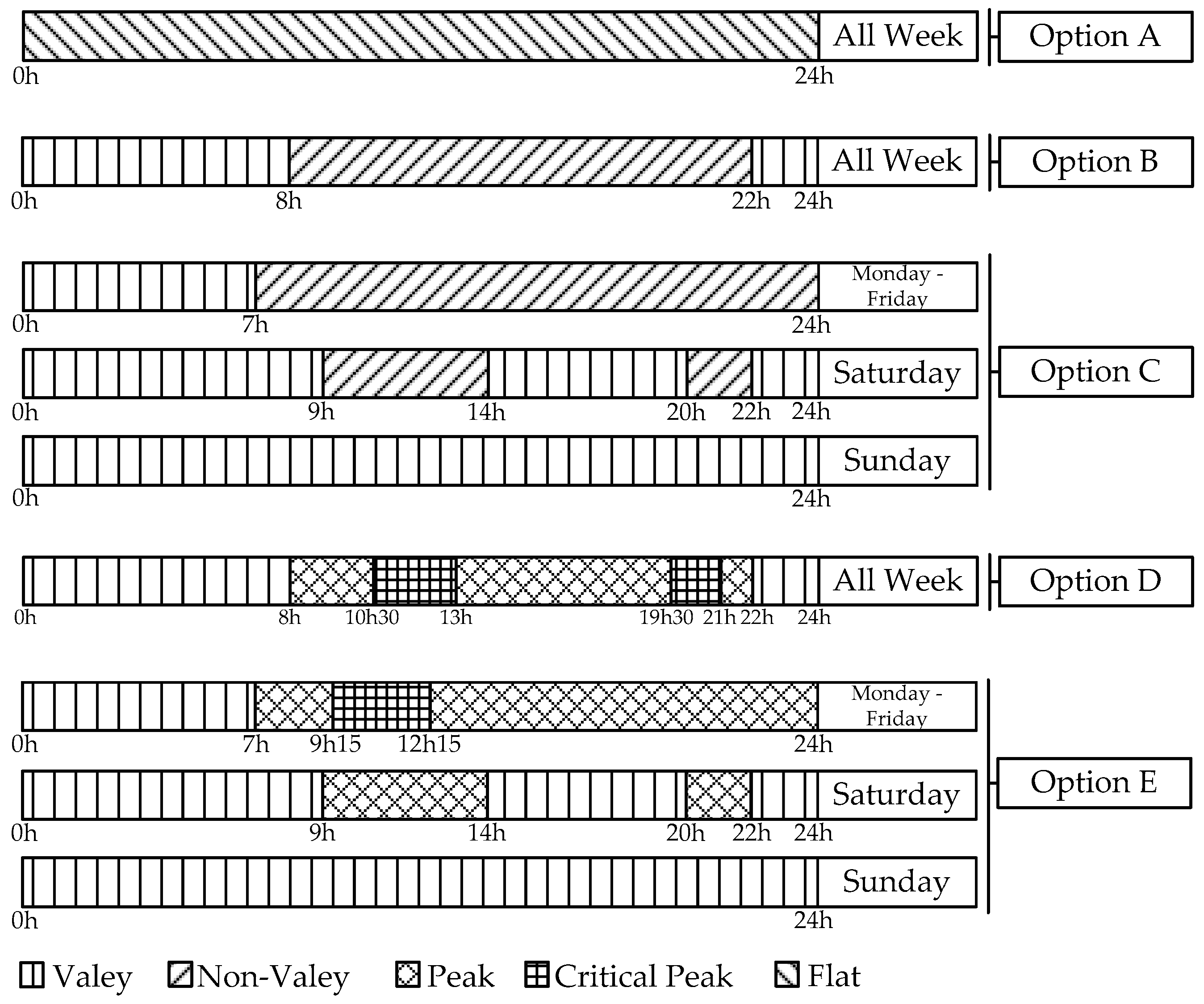
Figure 7 are shown five ToU rate options that are the real ones presently put into force by the Portuguese electricity retailer. The typical flat tariff of Portugal is represented in
Figure 7 by Option A; Options B and C are two tier ToU rates; and Options D and E are both three tier ToU rates. The evidence for the electricity ToU rates and price were withdrawn from [
46]. These prices and ToU rates were put into force by the electricity retailer in 2016 for the Portuguese residential market [
46]. The maximum price at critical peak hours is 0.2668 €/kWh as it can be witnessed by noticing in
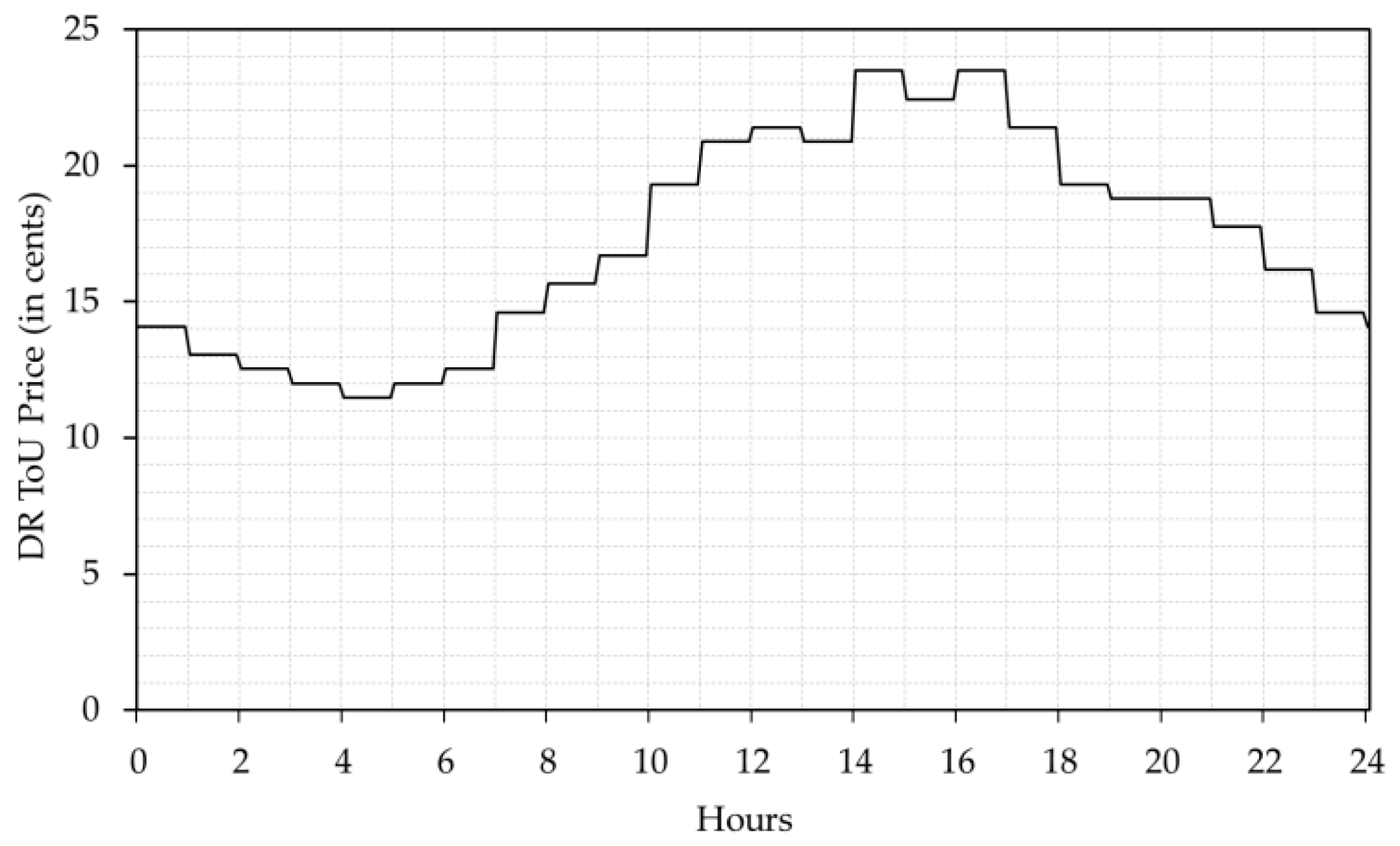
Table 1 and this price is only as high for the three tier ToU rates. The bottom price value can be found in both two and three tier ToU rates with 0.1232 €/kWh and is the price assigned to the valley hours. In this study, another tariff option was taken into account representing a price signal for each hour of the 24 h of the optimization horizon—Option F—which was adapted from [
64]. The intent is to verify if this option behaves better than the abovementioned existing options and it can be observed in
Figure 8.
4. Result Analysis
By considering all existing ToU rates by the Portuguese electricity retailer for the residential sector, the consumed energy cost of the AC unit can be calculated once the performance regarding the consumption of energy throughout the whole week is assessed.
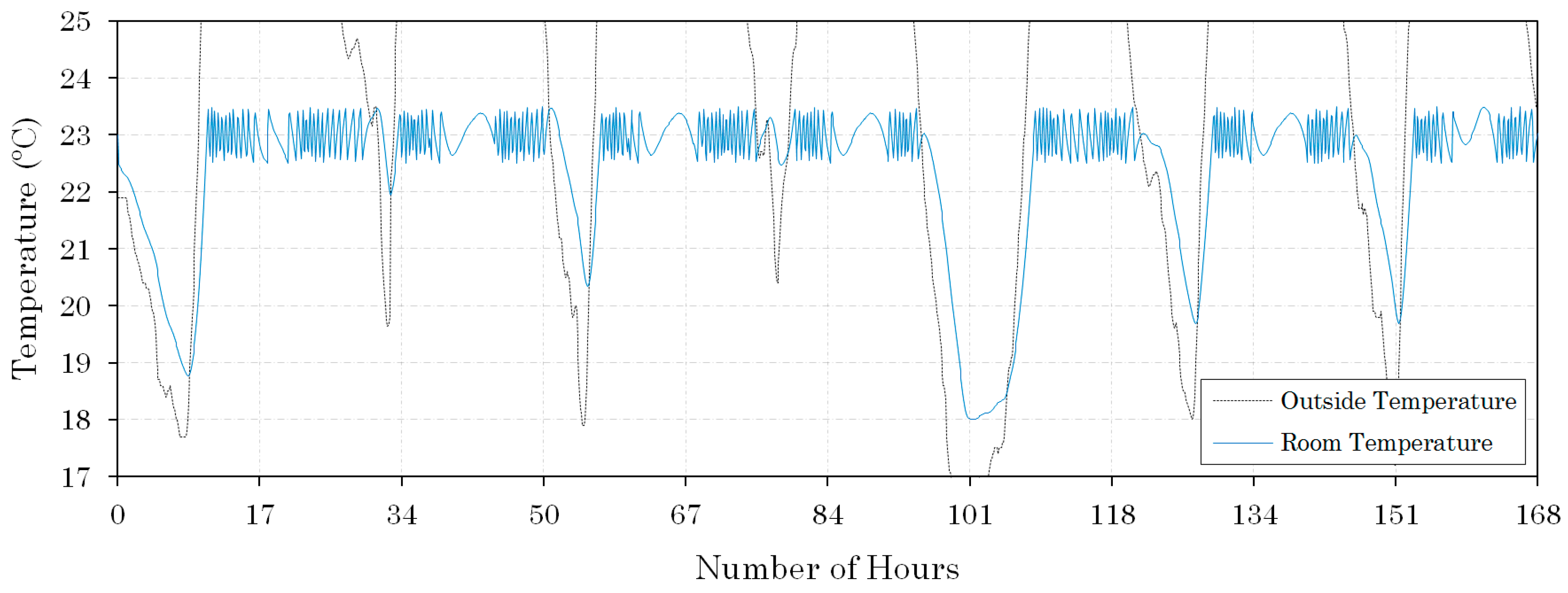
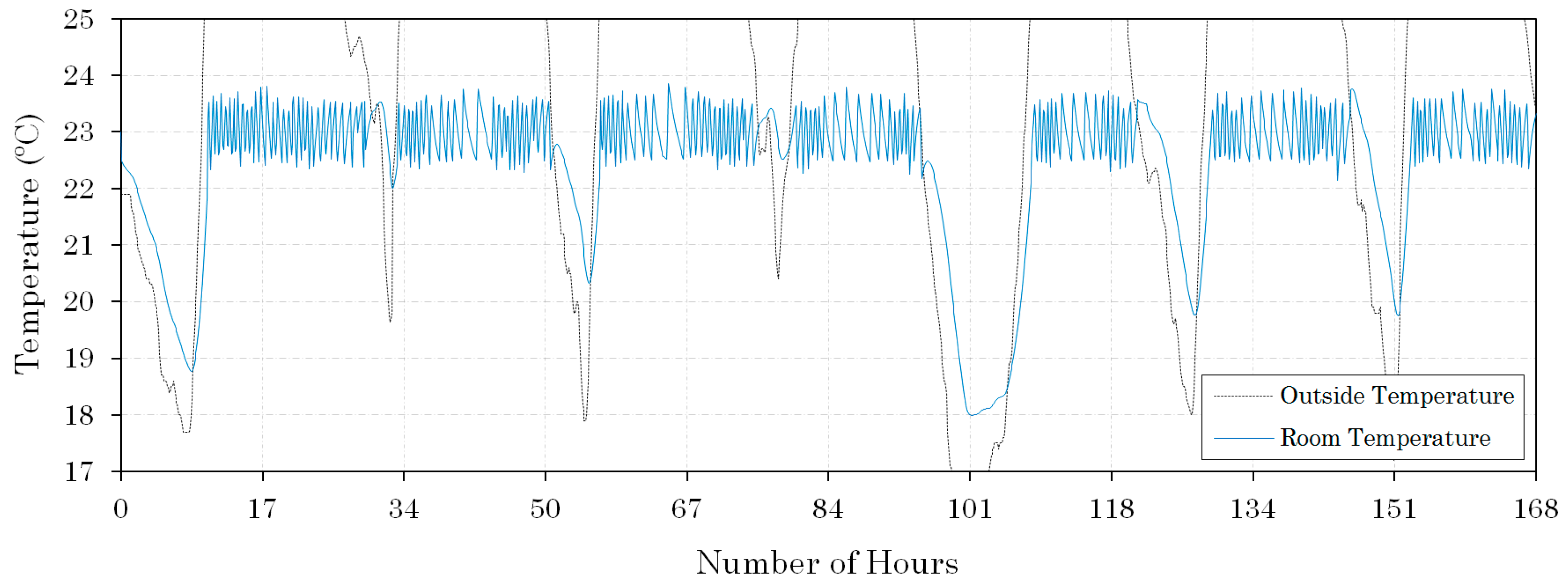
As stated throughout the paper, the performance of the ON/OFF, PID and MPC control methods of the air conditioning (AC) of the room is simulated and later compared. As expected, as these three control methods are rather different, the behavior of the temperature of the room will be somewhat different as well. The behavior of the room’s temperature for all three control options during the entire week can be observed in
Figure 9,
Figure 10 and
Figure 11.
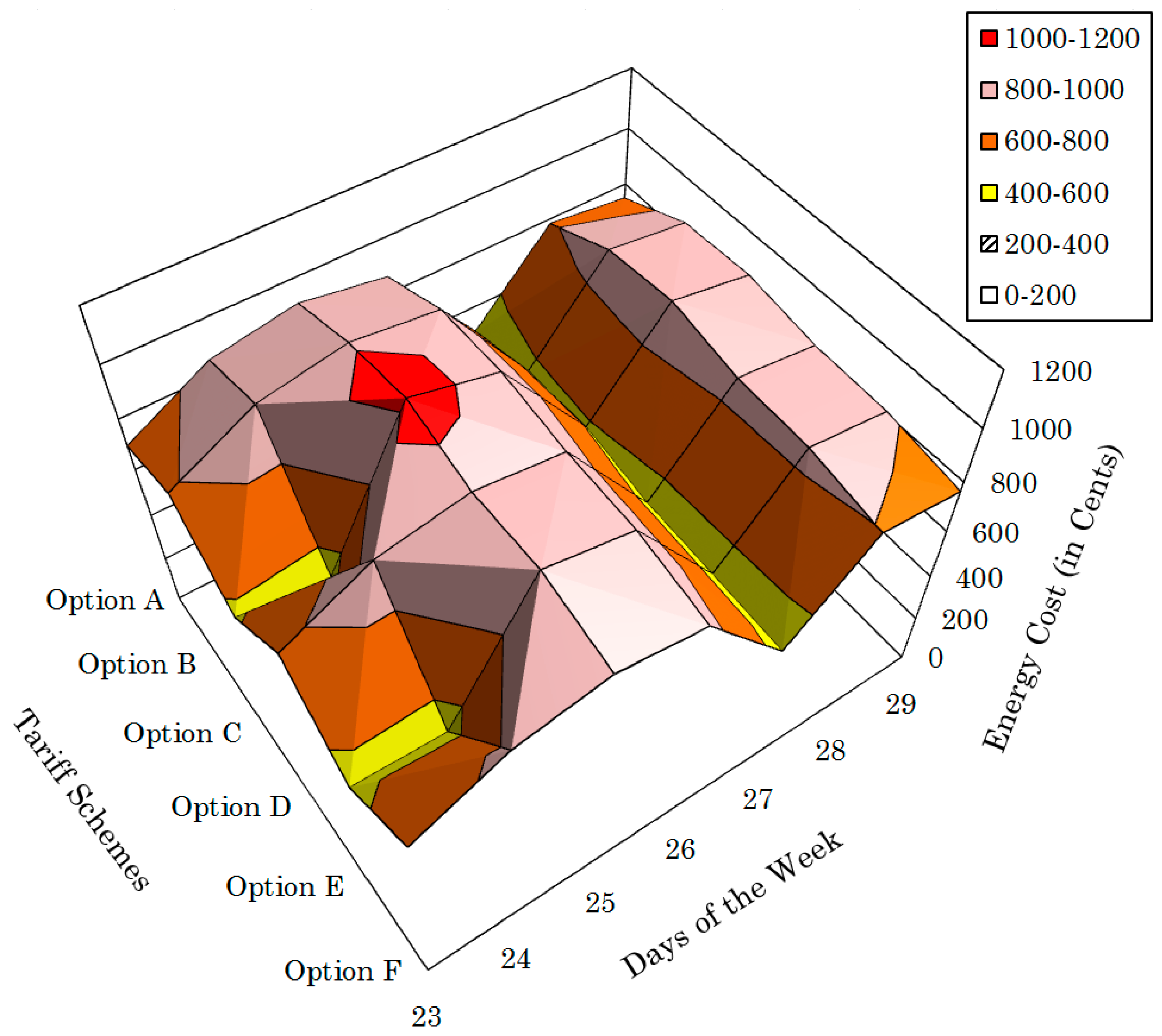
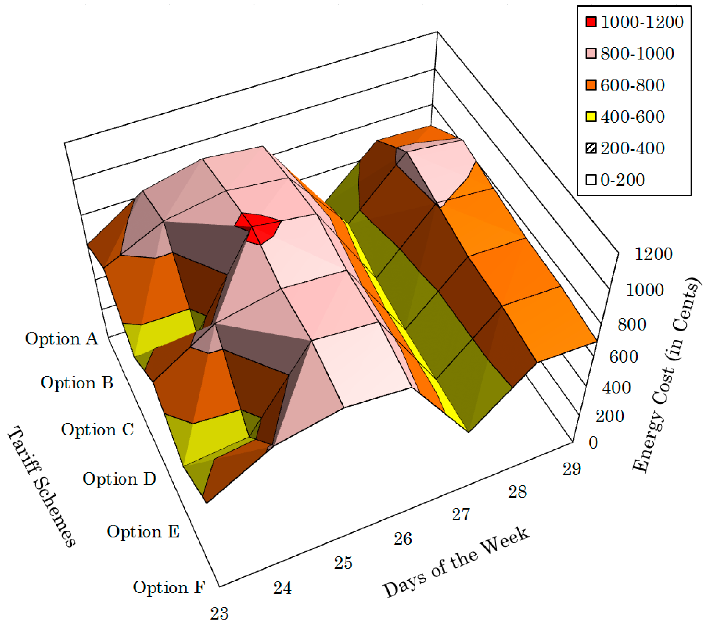
The results of the cost of the used energy by the AC unit of the three control options in cents under the six ToU rates can be observed in
Figure 12,
Figure 13 and
Figure 14. Through a careful analysis of
Figure 12,
Figure 13 and
Figure 14, it can be assessed that the cost of the consumed energy by the AC unit, in cents, is lower if controlled by the MPC method to the detriment of other control methods. As evidence, it can be observed in
Figure 14 that on 27 July the AC unit consumes less energy when compared to the remaining control methods for the same day. This is expressed visually since for this day the cost for energy is in the area of 200–400 cents for all the six ToU rate options.
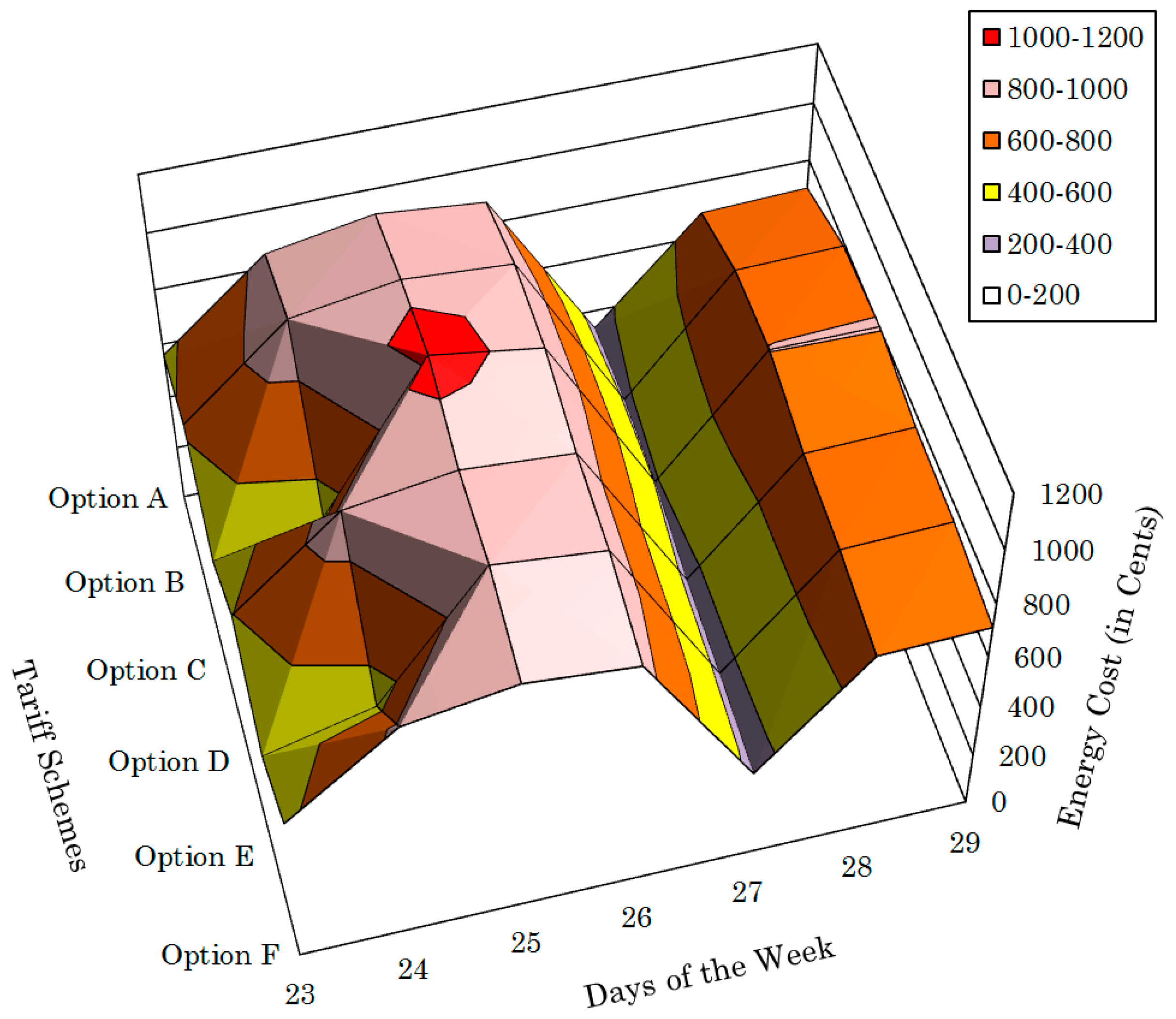
By comparing
Figure 12,
Figure 13 and
Figure 14 for the remaining days, it can be seen that the costs appear to be similar. However, on 25 July, the PID control option turns out to be the most economical one.
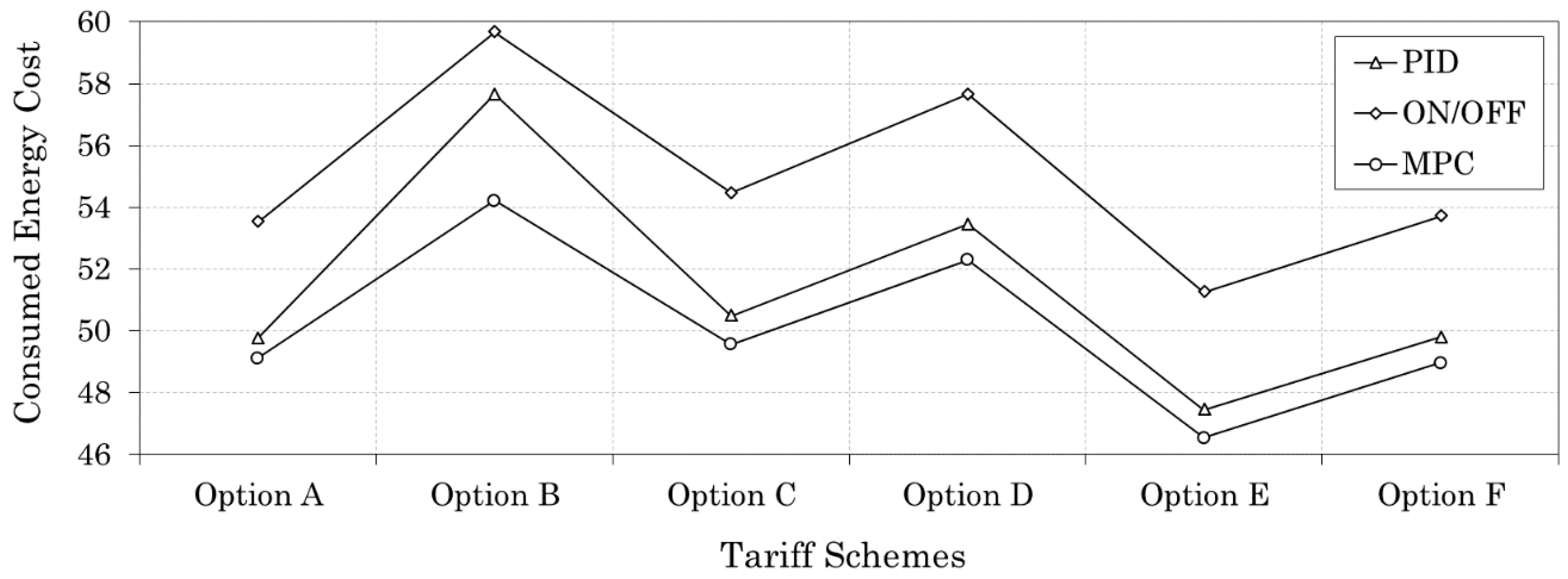
In
Figure 15, the complete results of the entire simulation of ON/OFF, PID and MPC control methods can be observed, under all the six options of ToU rates. By cautiously analyzing
Figure 15, it can be inferred that the MPC option has shown the best performance among the considered control methods. By analyzing this figure, it can also be concluded that tariff option that guarantees the lowest cost is Option E—a three tier ToU rate that gives lower prices during weekends. By continuing to examine the obtained results shown in
Table 1, it can also be noticed that the ON/OFF happens to be the control method with the highest associated cost between the three control options. This observation can also be confirmed in
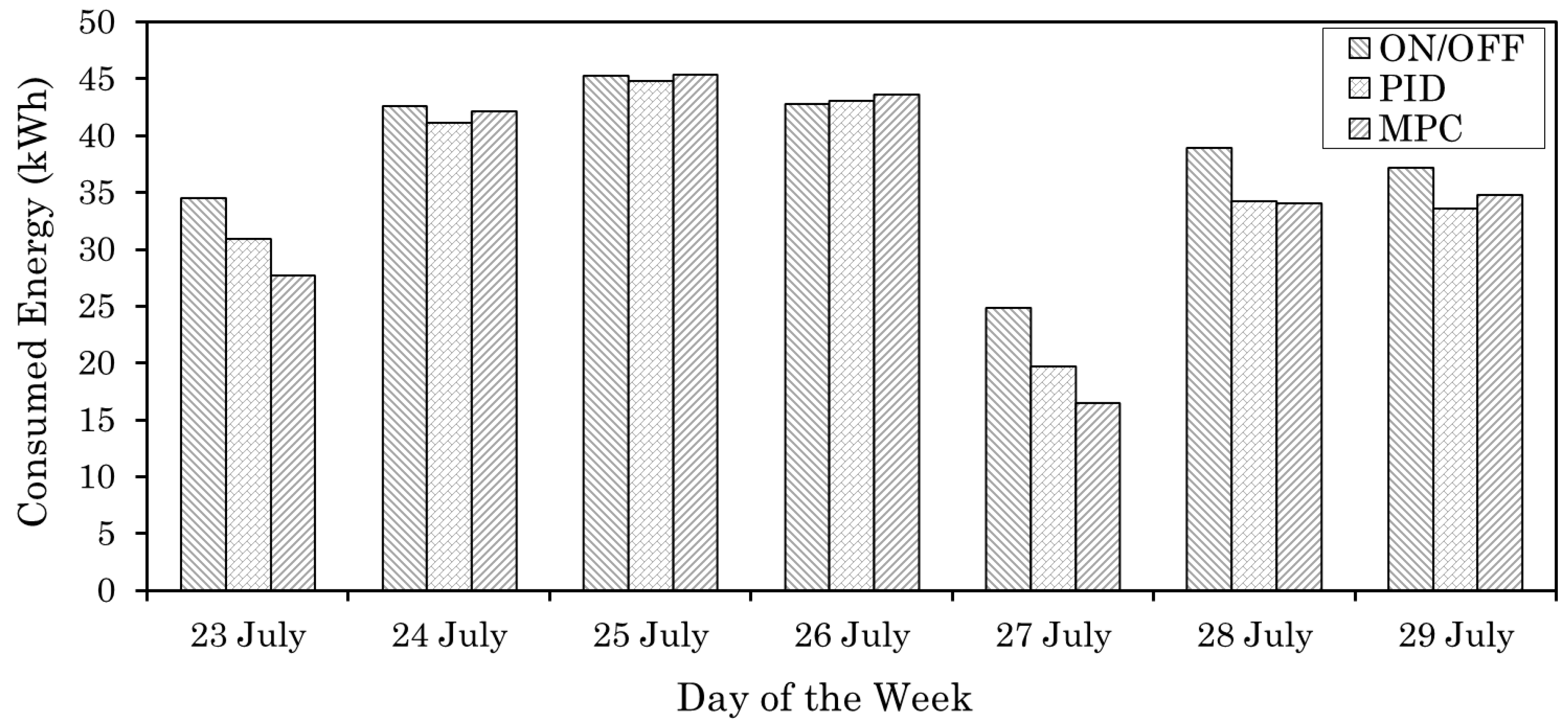
Figure 15. This figure not only confirms that the MPC is the best option for the consumer but also confirms that the ONN/OF is by far the priciest one, with PID being close to the MPC. By quantifying exactly how much can be save by opting for the MPC, the results show with this control method it is possible to save 9.2% when compared to the conventional ON/OFF, while with the PID it is possible to save 7.4% when also compared with ON/OFF. Even though the PID control option shows better performance regarding the energy consumption during a few days of the week, as can be seen in
Figure 16, the results show that the MPC performs better when compared to the PID by saving 1.8% in cost. This occurs because the MPC considers the price signal and during periods of the day when the cost is lower. Thus, in thes cases, the MPC allows the consumption of more energy without compromising the overall cost.
The results have shown that the option that allowed a price signal for the 24 h of the optimization horizon released by the retailer—Option F was still the second best tariff option and was surpassed only by tariff Option E since this option allowed much lower prices during the weekend. However, by selecting ToU Option F, the results show that the consumer spends just 5.2% more when compared with Option E—the optimal solution for the customer. By further analyzing
Figure 15, it can be observed that the most expensive option happens to be Option B which is a two tier ToU rate that never changes throughout the whole summer, being a working day or not. To emphasize how much the consumer can save by selecting the best AC unit control option and ToU rate, the results show that up to 14.2% can be saved by electing ToUOption E rather than Option B, the costliest one.

 ,
, 


