Abstract
Finding efficient and accurate solution methods for nonlinear equilibrium equations is a challenging task. This is the case of systems with friction-induced nonlinearities, e.g., friction-damped turbomachinery assemblies and automotive applications such as brakes. In order to tackle this strategic task, several methods have been developed, both in the time and in the frequency domains. Time marching methods are regarded as the most accurate option, but their computational cost becomes prohibitive when friction nonlinearities are present. This poses a problem in all those cases where alternative frequency domain methods cannot be applied effectively, e.g., if transients, non-periodic excitation/solution, or highly nonlinear systems are of interest. The purpose of this paper is to propose three independent methods to make time-marching more competitive. Two of these methods can be applied to any existing direct integration scheme with minimal adjustments, but the computational time cut they introduce is significant. The last method is instead tailored for systems where the inertia force contribution is negligible. All methods are thoroughly validated numerically using a standard Newmark- integration scheme as a reference.
1. Introduction
Frictional interfaces can be found in numerous aspects of everyday life: brakes in the automotive sector [1], joints in most engineering structures [2], friction damping devices in turbines (for energy production and aircraft engines alike) [3], and so on. Friction damping devices on turbine disks, either as integral parts of the disk (e.g., shrouds) [4,5,6] or as separate components [7,8,9,10,11,12,13], are considered strategic in the field, as, if well designed, they can play a key role in avoiding high cycle fatigue failures caused by large resonant stresses [2,3,14,15].
A trustworthy design of structures with friction interfaces entails finding:
- a reliable model for the force-displacement relation at the contact interface;
- an efficient yet accurate technique to solve the nonlinear equilibrium equations that obtain the nonlinear response in a timely manner, compatible with design purposes.
Point 1 has been addressed by several authors, leading to different contact models and techniques. Some authors adopt a dynamic Lagrangian method to solve the contact patch [16,17], i.e., the contact constraints are taken into account in their non-regularized form without additional compliance. Other authors, e.g., [12,13,18,19,20], apply a “spring-slider” contact element [3,21,22,23] to each meshed node belonging to the contact area, introducing normal and tangential stiffnesses and a Coulomb friction law. In detail, the contact interactions can be geometrically divided in normal and tangential directions. A unilateral contact law is often considered in the normal direction (with or without normal contact stiffness ), and frictional law for the tangential contact. This last method is here preferred, as its calibration parameters (, and ), however difficult to determine, represent a physical measurable property [24,25,26,27,28,29]. These contact elements belong to the larger family of heuristic models, as opposed to microscale “realistic” models, where asperities and surface roughness are modeled using stochastic distributions [30]. Heuristic models are here preferred because of their simplicity, because of the ease of calibration, and, most importantly, because they have proven their adequacy in several experimental/numerical comparisons [31,32]. In detail, this paper makes use of a 3D contact model [18,22], most often applied because of its versatility. It should be noted that all the techniques here developed can be applied to any contact model belonging to the “spring-slider” family with minor adjustments. As for Point 2, the presence of friction-induced nonlinearities makes standard solution techniques (typically applied in commercial FE codes) inadequate. Whenever possible, the response is assumed to be periodic so that harmonic balance methods (HBMs) can be used in the frequency domain to compute the steady-state response [33,34,35,36,37]. It should be noted that the HBM is an approximate method [38]. In linear systems, the harmonic support is easily determined by the harmonic content of the forcing function (e.g., mono-harmonic). However, if nonlinearities are present, higher-order harmonics may need to be included to ensure a proper representation of friction forces and displacements, with a detrimental effect on the the computational time. Most importantly, the HBM cannot be applied effectively in all those cases where the response is non-periodic or the transient is of interest. This paper focuses on time marching methods, an alternative to HBM. Time marching methods start with an initial solution (defined at time zero) and march the equations in time while applying boundary conditions. Therefore, the solution is dependent on the solutions at previous times. An example of a time marching method is any direct time integration (DTI) algorithm, but additional alternatives will be explored within this work. The purpose of this paper is to provide a series of methods to make time marching methods competitive and practically applicable for design purposes, a result of strategic importance in all those cases where frequency-domain solution methods cannot be applied. This task will be carried out in a series of substeps outlined below.
- Section 2 will recapitulate the dynamic governing equations and will present the test case used as a demonstrator throughout this article.
- Section 3 will recapitulate the main features of the contact model and present an alternative way to represent contact forces, as a sequence of linear states.
All proposed methods will be validated and time savings will be quantified using a reference test case as a benchmark. Their applicability to different fields and situations will be discussed.
2. Governing Equations
All multi-degree of freedom (multi-DOF) systems subjected to an external dynamic forcing and to friction share similar equilibrium equations. In the time domain, they can be written as
The dependence of the contact forces vector from the vector of displacements is defined by the contact model [18,22], further discussed below.
Equation (1) can be tailored to represent an underplatform damper inserted between two adjacent turbine blades. The dissipative function of underplatform dampers has been discussed in the introduction, while Figure 1 shows a graphical representation of a turbine disk with underplatform dampers.
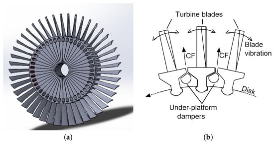
Figure 1.
(a) CAD model of a turbine bladed disk with underplatform dampers (not directly visible in the figure). (b) Sketch representing a close up of three blades with interposed underplatform dampers.
The numerical code concerned with the solution of Equation (1), already applied and validated in [38,39], can be considered as a “plug-in” software used to represent any given underplatform damper between blades modeled using finite elements (see also Figure 2a). The damper is here considered as a rigid body. The rigid body assumption is well justified by the bulkiness of “solid-bar” underplatform dampers and has already been validated against specific experimental evidence on underplatform dampers and blades [23,31,32]. The same conclusion has been drawn for similar applications in [4]. Furthermore, this choice has two advantages: (1) damper mass, shape, and contact points are easily editable by the user, and (2) the number of physical damper DOFs is limited, regardless of the selected number of contact points.
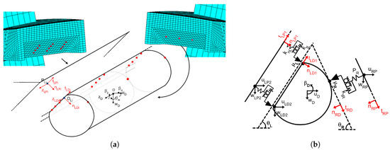
Figure 2.
(a) Contact model with three contact springs. (b) Contact patches on the blade platforms and on the strip damper.
In this paper, the system is further simplified, to be easily used as a demonstrator. A 2D version of the damper between a set of blades is considered, as shown in Figure 2b. This version of the damper system has been effectively used and validated in a series of previous works [19,39,40], where the blade platforms undergo bending (i.e., pure in plane) modes of vibration. Furthermore, it should be noted that the techniques described throughout Section 3, Section 4 and Section 5 can be easily extended to more complex systems. Their formulation is general.
With reference to Figure 2b, Equation (1) becomes
where is the mass matrix, is the vector of external forces on the damper, is the vector of unknowns at the damper center of mass, and is the vector of input platform displacements, where . The vector is here seen as an input because it comes from the displacement of the nodes on the blade platforms, provided by “higher-level” software [38] concerned with the blades’ dynamics. The indication of the time instant has been dropped for the sake of brevity.
In this particular set of equations, there are no harmonic “external forces.” The input platform displacements act on the contact elements and produce the contact forces that serve as the harmonic external excitation to the system. Further details on the contact model implementation are given in Section 3. The vector of contact forces refers to the contact forces transposed at the damper center of mass:
is expressed in the global reference system, while , , and are expressed in the local reference system (in red in Figure 2b), specific for each contact point i.
Transformation matrices are used to switch between reference systems:
where is a 2 × 2 rotation matrix, and is a 2 × 3 transformation matrix.
3. The Contact Model and Its Piecewise Linearity
The contact forces at a particular instant in time and at a given contact node pair are computed starting from the relative displacements at the contact using a friction contact model with normal load variation that is widely used in the nonlinear forced response analysis of frictional constraint structures [18,22], see also Figure 3. The time-discrete implementation facilitates the contact model application in time-marching solution methods. The main drawback is that contact state transitions are captured with finite accuracy, i.e., the length of the chosen time step . This has, however, negligible effects on the solution for the range of investigated .
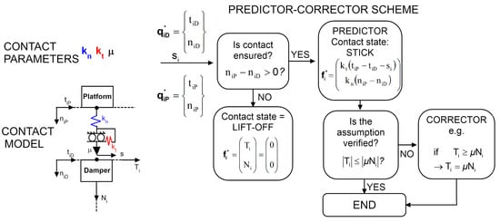
Figure 3.
(Left) Contact model representation and list of its calibration parameters. (Right) Standard implementation of the contact model routine through a predictor-corrector scheme.
Figure 3 shows the contact element in case of 2D motion. In case of 3D motion, e.g., see Figure 2a, it is assumed that the in-plane tangential components of the contact force are independent from each other (i.e., quasi-3D). In other words, an uncoupled in-plane motion/force coordinate, here termed , orthogonal to , is added. This assumption is commonly used in the calculation of the nonlinear forced response of structures with frictional constraints, see [20,41,42,43]
Each contact element can undergo, alternatively, three different contact states.
- Lift-off: There is a gap between the platform and damper contact points (i.e., ), and contact forces are null .
- Stick: There is interference between the platform and damper contact points (i.e., ). Furthermore, tangential relative displacement is limited, and a proportional relation between tangential forces and displacements exists: , where is the relative displacement of the tip of the slider with respect to the contact point on the damper.
- Slip: There is interference between the platform and damper contact points (i.e., ). Furthermore, the tangential relative displacement exceeds a threshold value, and a proportional relation between tangential and normal forces exists: .
The full set of conditions for the three contact states described above can be found in [11].
The standard implementation of this contact model sees a “black-box-like” subroutine, which receives as input the displacement vectors , at the time step and the slider displacement at time and gives, as output, the contact forces . Inside the sub-routine a predictor-corrector scheme (see Figure 3) checks the inputs against a series of “conditions” in order to assign the correct contact state and the corresponding values of contact forces.
This paper proposes a novel alternative to implementing the contact model constitutive equations. The contact state transition conditions and contact forces expressions are unchanged, so the ultimate result is the same. However, this novel formulation brings out an important feature of the chosen kind of contact model: nonlinearity is obtained through a time sequence of linear systems. The nonlinear system is actually a piecewise-linear system.
With reference to Equation (3), let us consider a specific instant in time. The local vector of contact forces is substituted by the product of the contact stiffness matrix and the vector of local relative displacement at the contact , plus a contribution from the slider.
The local contact stiffness matrix and the slider contribution change their configuration with the contact state, as described in Table 1. Therefore, if one considers a time interval during which the contact state of all the contact points remains unchanged, the system is perfectly linear. If the reader compares this formulation with the standard constitutive equations of the contact model, he/she will find the same ultimate result.

Table 1.
Expression of the contact stiffness matrix depending on the contact state.
4. Direct Time Integration Tailored to Systems with Friction Nonlinearities
In numerical analysis, numerical integration constitutes a broad family of algorithms for calculating the numerical value of a definite integral. By extension, the term is also used to describe the numerical solution of differential equations.
These methods rely on discretizing the continuous problem, i.e., ordinary differential equations (ODEs) such as Equation (1), since only rarely can it be solved analytically.
This involves, after the solution is defined at time zero (i.e., initial conditions), the attempt to satisfy dynamic equilibrium at discrete points in time. Most methods use equal time intervals at , 2, ..., N. However, this is not mandatory; in some cases, a variable time step might be employed. An example will be given in the following paragraphs.
4.1. Selection of the Direct Time Integration Method
An overwhelmingly large number of algorithms has been proposed over the years with varying degrees of complexity, accuracy, and computational cost. It is sometimes difficult to understand which algorithms are better suited to a given purpose. Appendix A.1 presents a classification of all families of DTI methods available in the literature. The classification highlights the aspects relevant to the problem at hand (the solution of 2nd order ODEs), thus allowing for an informed choice.
The algorithm used in this work is the Newmark- method, i.e., the constant average acceleration method [44]. It was chosen for the following reasons:
- it is reasonably accurate, especially for small , and does not introduce spurious damping and period elongation;
- it is suited for 2nd order ODEs, and no further processing is required;
- the method is implicit, which has a positive impact on the required time step size and on stability.
4.2. Adaptive Time Step Selection for Direct Time Integration Methods
As stated in [44], stability, convergence, and accuracy all depend on the size of the time step . Specifically, the chosen Newmark- method has the limitation to ensure convergence. The quantity is defined as the shortest natural period of the structural system, which is computed through a standard eigenvalue analysis.
Remark 1.
When computing , one should not consider the “structural” stiffness of the system but rather the complete effective stiffness, contact springs included (see Section 3). In other words, the value of changes with the contact state.
This aspect is not stressed in the few publications where the DTI of friction-damped turbo-machinery systems is carried out. One way to define a value of valid for all instants of the period of vibration is to use the highest effective stiffness that might be encountered, i.e., a full-stick state. With reference to Equation (2), the eigenvalue problem from which is defined is
where all () matrices have the “stick” configuration shown in Table 1. In this case, the structural stiffness matrix is not present because the damper is modeled as a rigid body. If it were, the overall stiffness matrix would be . Typical values of the contact springs, i.e., N/m, unfortunately produce 1 s. This makes DTI cumbersome, especially at low frequencies.
The reader will have noticed that the “effective stiffness” of the system changes with time (i.e., with the contact state). Therefore, the limit on depends on the specific contact state as well. For this reason, it is here proposed, as shown in Figure 4, that the time step is adapted to the contact state. The contact state is initially assumed to be equal to the previous one, i.e., : this value is fed into the integration scheme and produces the tentative value of the vector of displacements . The contact model run at instant with produces a given contact condition and, consequently, the time step . If , the algorithm goes on; otherwise, the time step is updated; if , the Newmark algorithm is re-executed with the updated value of . There are typically a few transitions per period of vibration (i.e., 4–7). The time savings are quite consistent: the signal shown in Figure 4b is in full slip condition for 54% of the total period of vibration. If it is run with a unique time step compatible with the full stick condition, it will take 187 time steps to complete. The adaptive algorithm reduces this number to 148. The “relative” time step savings in the investigated cases are in the 20–40% range compared with the standard condition. These values depend on the amount of gross slip/contact point detachment and on the values of contact parameters. These results have been obtained using parameters experimentally estimated in [29].
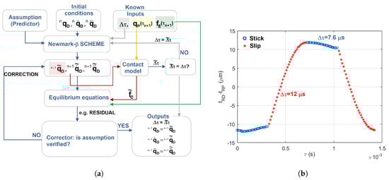
Figure 4.
(a) Scheme representing the Newmark- implicit DTI scheme (standard implementation) with an adaptive time step. (b) Example of result of Newmark- DTI with adaptive time step.
The adaptive time step can be applied to any DTI algorithm (e.g., Runge–Kutta and Euler) since all methods have limitations on .
4.3. A Novel “Piecewise-Linear” Implementation for Direct Time Integration Methods
Figure 4a clearly shows that, since Newmark-β is an implicit scheme and the system at hand is nonlinear, an initial assumption on one of the unknown vectors at time , e.g., is required. The first version of the damper model presented in [11] assumes . In other words, it assumes that the displacement keeps constant over a period . This assumption is not relied upon, as shown in Figure 4a and Appendix A.2: a predictor-corrector scheme (different from the one previously mentioned for the contact model) iterates until the assumed value is verified by the equilibrium equations. This assumption results in an average of ≈5 iterations per time step for frequencies <100 Hz and reaches as high as ≈11 for frequencies ≥200 Hz (see Figure 5a). Therefore, the impact on the computational time is quite negative and non-negligible. One may argue that better assumptions should be tried out, e.g., using the result of an explicit method as a starting guess. Many options have been tried out and the novel method proposed below was found to be the most suitable for our purpose: the number of iterations per time step is minimized thanks to an “ad-hoc” predictor-corrector.
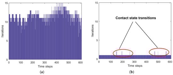
Figure 5.
Histogram representing the number of iterations per time step of the predictor-corrector scheme implemented in the DTI algorithm: (a) constant displacement assumption; (b) unchanged contact state assumption.
The novel initial assumption (i.e., predictor) is based on two strategic observations:
- the contact state changes only a few times per period of vibration (4–7 in cases encountered in this work);
- if the contact state does not change from time step to , the system can be considered perfectly linear (see Section 3)
This novel formulation manages to derive a tentative value of all unknown vectors using the piecewise linearity of the contact model (Section 3), i.e., setting . If the assumption is verified (i.e., the contact state is unchanged), as is the case in >90% of cases, only one iteration is required for each step. If it is not, then the procedure is repeated using, as an assumption, the updated matrices corresponding to the forecast contact state. Typically, only one additional iteration is required (see Figure 5b). The complete formulation is reported in Appendix A.2.
In other words, the Newmark- method is applied as if on a linear system for the entire duration of a given contact state (therefore, no iterations are required as described in [45]). Iterations are necessary only when a contact state transition occurs.
The overall computational time is reduced by a factor of almost 50%, e.g., for a 100 Hz 3-period DTI run, the “standard” algorithm’s the total time is 9.46 s, compared to the 5.09 s of the “Piecewise linear” implementation. Similar time savings have been found using different DTI integration schemes. Furthermore, it should be noted that this piecewise-linear implementation can be applied together with the adaptive time step to further increase time savings.
5. A Time-Marching Method for Systems with Negligible Inertial Effects
The concept of piecewise linearity of Coulomb friction contacts has secured significant improvements in the field of DTI algorithms and their implementation. Despite the improvements detailed in Section 4, the limitations on the value of the time step s may still be forbidding in many applications.
It will be shown below how it is possible to reduce the computational time by more than one order of magnitude in all those cases where inertial effects are negligible. A typical example is an underplatform damper between a set of blades or a flexible strip damper [46,47] in the same condition. Alternatively, brake systems where decelerations produce forces that are negligible with respect to friction forces can be studied using the same algorithm. This paper will focus on the first example to develop a novel quasi-static solution method.
5.1. The Influence of Damper Dynamics on the Overall Damper Equilibrium
The equations solved through DTI are dynamic equations; i.e., they take into account inertial and viscous damping effects. However, given the reduced mass of the damper and the lack of a damping matrix , it is worth investigating what role the dynamics inside Equation (2) play and what the consequences of neglecting it are. Furthermore, in many applications, the presence of a viscous damping matrix can be neglected as the damping provided by friction is far larger.
To properly answer the questions posed above, two aspects have to be considered:
- the magnitude of the damper inertia forces;
- the damper “inner resonance” (i.e., the natural frequencies of the damper oscillating on the contact springs).
To tackle the first point, let us consider a damper of mass . Both the centrifugal force (and therefore the contact forces) and the inertial effects are proportional to the mass of the damper; specifically, the centrifugal force is , and the inertial effects are , where is the rotation speed of the bladed disk, and is the frequency of vibration, i.e., close to the mode under investigation . Let us define a ratio between the two quantities:
It should be noted that this ratio does not depend on the mass of the damper. Let us consider a damper mounted on a turbine for energy production; it is therefore reasonable to set 3600 rpm and 0.5 m. Based on the authors’ experience, the magnitude of the damper displacement is at most m. In this specific case, the frequency of vibration (i.e., the mode being excited) would have to be >30 kHz in order to have the inertial forces at least 5% of the centrifugal force (i.e., ). Consequently, the damper vibrating with the first modes of a bladed system, typically in the range of 150–600 Hz, will not be affected by the inertia forces. This aspect allows for the safe reconstruction of the damper equilibrium starting from experimental data at low frequencies [11,19,29] and at higher realistic frequencies (i.e., 200–500 Hz) [39,40]. Regarding the damper inner dynamics, the presence of the contact springs causes high-frequency oscillations of the damper: they are visible as superposed waves in Figure 6. The frequency of oscillation , given by the mass of the damper (12 g in this example) and the values of contact springs (determined in ), is, in this case, ≈10 kHz.
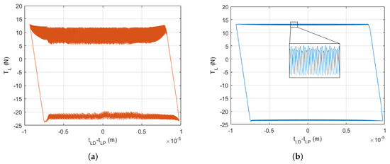
Figure 6.
(a) Low frequency hysteresis cycle at the left contact obtained through DTI without additional post-processing. (b) Low frequency hysteresis cycle at the left contact obtained through DTI and an a posteriori low-pass filter.
These oscillations are perfectly explained and predictable from a purely numerical point of view. However, they have not been encountered experimentally at either low [29] or higher frequencies [38,39,40]. For this reason, they must be removed “a posteriori” in order to make results more legible. This can be done only when the damper internal resonant frequency is far from the mode of vibration of the blades , i.e., for 1 kHz.
Remark 2.
Both and refer to modes of vibration of the blade/damper coupled system, but at the blade is vibrating (e.g., bending mode) and “driving” the damper with it. At , the blade itself may be far from its resonance (low mobility), and the damper is vibrating on the contact springs (local mobility mode).
If , the oscillations mentioned above can be filtered out thorough a low-pass filter (see Figure 6).
Remark 3.
These numerical oscillations cannot be removed safely if , or, more generally, if a mode of vibrating high mobility for the blade is very close (or ≈ coincident) to a high mobility for the damper. Hysteresis cycles appear strongly distorted and hard to interpret: further numerical and experimental investigation on damper–blade dynamic coupling is needed. Since the frequency range typically investigated is Hz, the damper acts only as a “spring-coupling” to the bladed system, so its dynamics can be safely neglected.
5.2. Quasi-Static Solution Method
The negligibility of the dynamic portion of the damper equilibrium equations is confirmed by the results of a newly developed solution method, here termed “quasi-static.” In essence, the method, whose implementation algorithm is reported in Appendix A.2, solves a modified version of an equilibrium equation given above (Equation (7)):
The strict limitations on the value of ( s) in DTI algorithms are caused by the damper internal resonance, i.e., the stability and convergence of the algorithm can be ensured only if these high-frequency oscillations are correctly captured. However, these oscillations, which are not observed experimentally and may be an artifact due to an imperfect method chosen to model the contact, are of no interest to the designer, especially in the early design stage.
If one choses to neglect the inertial terms from the equilibrium equation, then
- the spurious numerical oscillations will disappear (see Figure 7), and
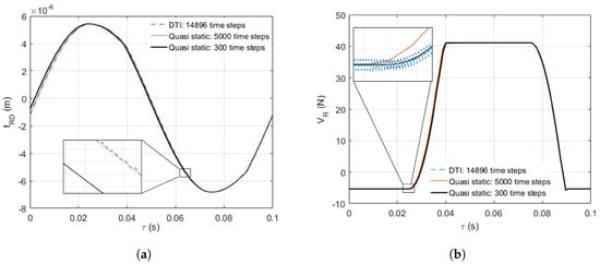 Figure 7. DTI vs. quasi-static results comparison. (a) Tangential displacement of the right damper contact point. (b) Vertical component of the right contact force.
 - inertial forces will cease to participate in the equilibrium, with negligible effects up to 30 kHz.
The time step used in this time-marching method is limited only by the precision the designer wants to obtain; i.e., if the user decides to discretize a period of vibration into 300 time steps, then a given contact state transition may be shifted by, at most, . Typical force and kinematic results of the quasi-static method are shown along with DTI results in Figure 7.
6. A Critical Comparison of the Proposed Methods
This section is concerned with offering the user practical guidelines and an indication of expected results when one of the three methods proposed in this paper is applied. In order to achieve this goal, a test case has been defined. The test case at hand sees an underplatform damper between a set of blade platforms (as shown in Figure 2b) vibrating at 200 Hz for one period of vibration. The blade platform kinematics is large enough to cause the damper to reach the bilateral gross slip condition (both the right and left interfaces are sliding). This results in six changes in contact states during one period of vibration. The resulting hysteresis cycle at the left (flat-on-flat) contact interface is shown in Figure 6.
The test case defined above has been solved using the following four methods:
- a standard Newmark- algorithm, as described in Appendix A.3, to be used as a reference case, which applies standard techniques and no particular adaptation to friction damped systems;
- a standard Newmark- algorithm with an adaptive time step (see Section 4.2);
- a piecewise-linear implementation of the Newmark- algorithm, as described in Section 4.3 and Appendix A.4;
- a quasi-static solution method, as described in Section 5 and Appendix B with a user-defined 300 time steps per period.
All methods yield the same set of results; forces and displacements are perfectly superposed. Accuracy is not impaired in the slightest by the proposed methods. Computational time, on the other hand, varies from case to case. The computational time needed for the case described in Method 1 is used as a reference to normalize other values.
As shown in Figure 8 all proposed methods lead to a non-negligible decrease in the computational time. The adaptive time step method (Method 2) introduces a 20% reduction in the computational time and can be applied to ALL existing DTI algorithms. It enables the user to automatically set the largest possible time step that still ensures convergence. Method 3 is instead applicable to all DTI methods and no restrictions on the test case are observed. It is especially useful for implicit algorithms (in this case, Newmark-) since it enables the user to make the best possible assumption when proceeding to the following time step (i.e., unchanged contact state) without unnecessary iterations. This leads to halved computational times. Methods 2 and 3 can be applied together, thus leading to an overall reduction in the computational time of ≈60%. The reader will notice that the quasi-static method (Method 4) reduces the overall computational time by more than one order of magnitude. This solution method, which is an alternative to DTI algorithms (and therefore to Methods 2 and 3) is, however, applicable only in those cases where inertial effects are negligible. When applicable, it is a very competitive alternative, especially in all those cases where displacements are large (leading to highly nonlinear systems) and the HBM needs large harmonic support, resulting in convergence issues.
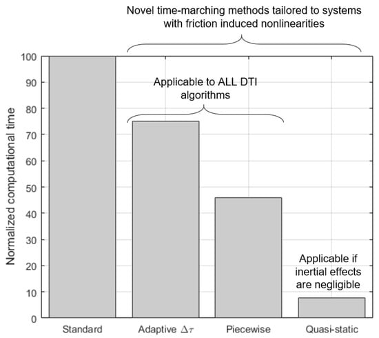
Figure 8.
Time savings introduced by the novel techniques and solution methods proposed in the paper. A standard Newmark- computation is taken as a reference.
7. Conclusions
Time marching solution methods are often regarded, especially in the turbomachinery field, as too cumbersome and therefore inapplicable to real industrial problems. This is especially true whenever nonlinearities, such as those induced by friction, are present. This paper proves that ad-hoc techniques tailored for the specific nonlinearity can make time-marching methods competitive.
All of them are based on one common idea: seeing the nonlinearity induced by friction as a time sequence of linear systems. As a result, only time steps corresponding to contact state transitions are truly non-linear. This idea has been applied to:
- the development of an adaptive time step selection for DTI algorithms resulting in a 20% decrease in the computational time;
- the development of a novel “piecewise-linear” formulation for the Newmark- scheme, adaptable to other DTI algorithms, and resulting in a 50% decrease in the computational time;
- the development of a novel quasi-static method to solve equilibrium equations where inertial effects are negligible, capable of reducing computational times by more than one order of magnitude.
The appendices to this paper offer a critical review of existing DTI algorithms that guide the reader through the selection of the most appropriate one for the specific test case at hand. Furthermore, they provide the reader with a step-by-step guide to the implementation of the three ideas outlined above. This constitutes, in the authors’ opinion, a considerable contribution in making time marching methods more applicable.
Author Contributions
The authors contributed equally to this paper.
Conflicts of Interest
The authors declare no conflict of interest.
Appendix A. Direct Time Integration
Appendix A.1. Classification of DTI Methods
It is difficult to find a classification of all families of DTI methods available in literature, even in specific text books on the subject [48]. For this reason, Table A1 presents a list that, although far from comprehensive, manages to group the most famous methods into “families” and highlights differences and similarities. The intended purpose is not to give formal definitions or proofs of concepts; rather, it is to highlight the choices that the user has to make when selecting and implementing a DTI algorithm.
Table A1.
Classification of main DTI methods.
Table A1.
Classification of main DTI methods.
| Optimized for 1st Order ODEs | for 2nd Order ODEs | ||
|---|---|---|---|
| General Multi-Steps | Runge-Kutta | Newmark’s Family | |
| Methods | Methods | of Methods | |
| Explicit | Forward Euler (I) | Classic (I-VIII) | Central Difference (I) |
| Adams-Bashfort (I-V) | |||
| Implicit | Trapezoidal Rule (II) | Constant average acc. (II) | |
| Backward Euler (II) | Linear acceleration (I) | ||
| Adams-Moulton (I–V) | Gauss-Legendre (II–X) | Wilson- (<II) | |
| Houbolt (<II) | |||
Algorithms developed for 1st order ODEs can be used to solve 2nd order ODEs, but this requires increasing the size of the system by a factor of two [49].
In principle equilibrium equations, such as Equations (1) and (2), may be solved by any standard numerical integration scheme. However, efficiency and numerical efforts must be considered, and it is worth looking at special techniques of integration especially suited for the analysis of friction damped systems. To this purpose, the following paragraphs explore the different families of methods and discuss their pros and cons.
Appendix A.1.1. Methods for 1st Order vs. 2nd Order ODEs
The equations of motion to be solved in structural dynamics are 2nd order of the form:
similar to Equations (1) and (2). Therefore, the Newmark’s family of methods are better suited to the purpose. The other methods are instead suited to solve 1st order systems:
such as
However, if one defines an auxiliary variable , one can adapt Equation (1) to
This, however, entails solving a system twice the size of the original. For this reason, Newmark’s family of methods is usually preferred, as it is in this work, to solve structural dynamics equilibrium equations. Other methods such as 4th order Runge–Kutta have been applied to this specific problem and are sometimes used in this field for validation purposes [50] since they are already implemented in the Matlab environment. While their use for a one-time check is perfectly adequate, their implementation in codes run iteratively is here discouraged.
Appendix A.1.2. Explicit vs. Implicit
A scheme is said to be explicit when the evaluation of does not require the solution of any system of equations and can instead be deduced directly from the results at the previous time-steps:
The computer storage requirements are typically low, but their main drawback is the small time step required to ensure stability and accuracy. In the implicit schemes, the displacements and the velocities at the current time step are expressed not only in terms of the values of the previous time step but also in terms of the current time step.
In this second case, if the system is linear, the solution simply requires a matrix inversion, i.e., Equation (A6) is solved together with the reference equilibrium equations as shown in [45]. If the system is nonlinear, this is not enough: an iterative scheme, usually the Newton–Rapshon method, is required as well. Therefore, compared to explicit methods, the cost per time step is greater and more computer storage space is required. An advantage of implicit methods is the larger time step size allowed.
Appendix A.1.3. Stability, Accuracy and Convergence
Numerical methods for integrating equations of motion are compared in terms of their stability, accuracy, and convergence. In general, these properties depend upon the ratio of the time step, , to the shortest natural period of the structural system .
Stability is defined in a slightly different manner, depending on the family of integration methods, but its concept is associated “with the propagation of errors of the numerical technique as the calculations progress with a finite interval size, that is, what the effects of errors made on one step will have on succeeding steps,” as pointed out by Distefano [51]. Explicit numerical methods usually require smaller time steps in order to ensure stability, implicit numerical integration methods allow for values. In detail, all implicit Newmark’s methods in Table A1 are unconditionally stable.
By convergence, one means that the finite difference solution approaches the true solution as the interval size approaches zero . It should be clear from the above definitions that convergence does not necessarily imply stability, i.e., the Newmark- method is unconditionally stable but convergent only for [44].
The roman numerals in parenthesis in Table A1 represent the order of accuracy of the method, i.e., the truncation error between a “true” reference solution and that offered by the integration scheme is , where a is the order of accuracy. Therefore, the smaller the time step, the higher the accuracy for a given algorithm. Provided that convergence and stability limits are met, some methods ensure, for a given , lower truncation errors than others (i.e., 4th order Runge–Kutta vs. 2nd order Runge–Kutta): higher accuracy, however, also implies greater computational effort, e.g., 4th order Runge–Kutta requires four (vs. two) function evaluations per time step to achieve a truncation error .
In Newmark’s family of methods, accuracy is also measured in terms of period elongation and numerical damping [44]. Implicit methods such as Wilson- and Houbolt, which were derived from the classical Newmark’s constant average acceleration, are unconditionally stable but introduce ’distortions’ in the solution.
Appendix A.2. The Newmark-β Method
The Newmark method was originally introduced to solve second order differential equations arising from dynamic equilibrium in structural dynamics [44]. The Newmark method essentially approximates the velocity and displacement vectors at time using the following expressions:
where and in the Newmark- method to ensure stability and a lack of numerical damping [44]. It is clear that an assumption on one of the vectors (either displacement, velocity, or acceleration) at time must be made since this is an implicit scheme and the system is nonlinear. In detail, if the system was linear, e.g., , one would be able to find the correct solution in one iteration by solving a system composed of the equilibrium equation and Newmark’s constitutive relations, i.e.,
The system above has three equations and three unknowns, so the algorithm does not require any iterations. Unfortunately, friction introduces nonlinearity, so assumptions and a predictor-corrector method are required. The cleverness of the initial assumption and of the corrections operated can increase the algorithm efficiency by a factor of ≈2. The following subsections present and compare two alternatives: the standard all-purpose algorithm and one which was purposely developed for friction-induced nonlinearities.
Appendix A.3. Standard Implementation
This section presents the algorithm used in [11]. It is a classical implementation of the Newmark- method. The following makes reference to an equilibrium equation given above (Equation (2)):
- The values of , , , , and are known either from initial conditions or the previous integration step.
- PREDICTOR: An assumption on one of the unknown vectors at must be performed, e.g., is postulated.
- The values of and are computed using Newmark’s relations in Equation (A7) and the assumption at Step 2.
- Vector is transformed into local displacements at the contact using Equation (4). The same is done with the displacements of the platform contact points, thus obtaining .
- The vectors of local displacements at the contacts are fed into the contact model. Thus, the local vectors of contact forces are obtained and transformed into vector using the transformation matrices from Equation (4).
- The residual for Equation (2), also known as unbalanced force, is computed:
- The incremental displacement is computed:
- CORRECTOR: If the incremental displacement is below a given tolerance , then the equilibrium is satisfied and the integration goes to . Otherwise, the vectors of unknowns are corrected as follows (corrections factors derived from Newmark’s relations):
Appendix A.4. Piecewise Linear Implementation
This section presents the novel algorithm proposed in this thesis. The following makes reference to an equilibrium equation given above (Equation (7)):
- The values of , , , , , and the contact states’ effective stiffness matrices and are known either from initial conditions or the previous integration step.
- PREDICTOR: It is assumed that the contact state at is the same as that of the previous time step, i.e.,It is therefore possible to express a tentative version of the equilibrium equations at time as (see Equation (7)):Let us rename the following quantities for the sake of brevity:
- The system of equations composed of Equation (A13) and the constitutive Newmark relations Equation (A7) is solved. Below is the expression for :The expressions for and are computed using Newmark’s equations (Equation (A7)).
- Vector is transformed into local displacements at the contact using Equation (4). The same is done with the displacements of the platform contact points, thus obtaining .
- The vectors of local displacements at the contacts (of both the platforms and the dampers), together with the slider variable are fed into a function (similar to the contact element function) that checks whether their values are compatible with the postulated contact condition. In other words, for each i, whether the structure of and is compatible with the values of local platforms and damper displacements is checked (see Table 1).
- CORRECTOR: If the compatibility is verified, then the equilibrium postulated in Equation (A13) is indeed satisfied, and the integration goes to . In this case, all slider variables are updated according to the verified contact condition (, to be used at time step ).Otherwise, the structure of all effective contact stiffness matrices is updated according to the indications of the function mentioned at Step 5—see also Table 1:The algorithm is then repeated starting from Step 3.
Appendix B. Quasi-Static Method Algorithm
The following makes reference to an equilibrium equation given above (Equation (10)):
- The values of , , , , , and the contact states’ effective stiffness matrices and are known either from initial conditions or the previous integration step.
- PREDICTOR: It is assumed that the contact state at is the same as that of the previous time step, i.e.,
- It is therefore possible to compute the expression of using the tentative version of the equilibrium equations at time (see Equation (10)):where
- Vector is transformed into local displacements at the contact using Equation (4). The same is done with the displacements of the platform contact points, thus obtaining .
- The vectors of local displacements at the contacts (of both the platforms and the damper), together with the slider variable are fed into a function (similar to the contact element function) that checks whether their values are compatible with the postulated contact condition. In other words, for each i, whether the structure of and is compatible with the values of local platforms and damper displacements is checked (see Table 1).
- CORRECTOR: If the compatibility is verified, then the equilibrium postulated in Equation (10) is indeed satisfied, and the integration goes to . In this case, all slider variables are updated according to the verified contact condition (, to be used at time step ).Otherwise, the structure of all effective contact stiffness matrices is updated according to the indications of the function mentioned at Step 5—see also Table 1:The algorithm is then repeated starting from Step 3.
References
- Massi, F.; Baillet, L.; Giannini, O.; Sestieri, A. Brake squeal: Linear and nonlinear numerical approaches. Mech. Syst. Signal Process. 2007, 21, 2374–2393. [Google Scholar] [CrossRef]
- Brake, M.R. The Mechanics of Jointed Structures; Springer International Publishing: New York, NY, USA, 2018. [Google Scholar]
- Griffin, J. Friction Damping of Resonant Stresses in Gas Turbine Engine Airfoils. J. Eng. Power 1980, 102, 329. [Google Scholar] [CrossRef]
- Szwedowicz, J.; Secall-Wimmel, T.; Dünck-Kerst, P. Damping Performance of Axial Turbine Stages with Loosely Assembled Friction Bolts: The Nonlinear Dynamic Assessment. J. Eng. Gas Turbines Power 2008, 130. [Google Scholar] [CrossRef]
- Berruti, T.; Maschio, V. Experimental Investigation on the Forced Response of a Dummy Counter-Rotating Turbine Stage with Friction Damping. J. Eng. Gas Turbines Power 2012, 134, 122502. [Google Scholar] [CrossRef]
- Gastaldi, C.; Zucca, S.; Epureanu, B.I. Jacobian Projection for the Reduction of Friction Induced Nonlinearities. In Proceedings of the ISMA 2016, Leuven, Belgium, 19–21 September 2016. [Google Scholar]
- Šanliturk, K.; Ewins, D.; Stanbridge, A. Underplatform dampers for turbine blades: Theoretical modelling, analysis and comparison with experimental data. J. Eng. Gas Turbines Power 2001, 123, 919–929. [Google Scholar] [CrossRef]
- Panning, L.; Popp, K.; Sextro, W.; Götting, F.; Kayser, A.; Wolter, I. Asymmetrical Underplatform Dampers in Gas Turbine Bladings: Theory and Application. In Proceedings of the ASME Turbo Expo 2004: Power for Land, Sea, and Air, Vienna, Austria, 14–17 June 2004. [Google Scholar]
- Berruti, T.; Firrone, C.M.; Pizzolante, M.; Gola, M.M. Fatigue Damage Prevention on Turbine Blades: Study of Underplatform Damper Shape. Key Eng. Mater. 2007, 347, 159–164. [Google Scholar] [CrossRef]
- Sever, I.; Petrov, E.; Ewins, D. Experimental and Numerical Investigation of Rotating Bladed Disk Forced Response Using Underplatform Friction Dampers. ASME J. Eng. Gas Turbines Power 2008, 130. [Google Scholar] [CrossRef]
- Gola, M.; Liu, T. A direct experimental-numerical method for investigations of a laboratory under-platform damper behavior. Int. J. Solids Struct. 2014, 51, 4245–4259. [Google Scholar] [CrossRef][Green Version]
- Afzal, M.; Arteaga, I.L.; Kari, L. An analytical calculation of the Jacobian matrix for 3D friction contact model applied to turbine blade shroud contact. Comput. Struct. 2016, 177, 204–217. [Google Scholar] [CrossRef]
- Pesaresi, L.; Salles, L.; Jones, A.; Green, J.; Schwingshackl, C. Modelling the nonlinear behaviour of an underplatform damper test rig for turbine applications. Mech. Syst. Signal Process. 2017, 85, 662–679. [Google Scholar] [CrossRef]
- Petrov, E.; Ewins, D. Effects of Damping and Varying Contact Area at Blade-Disk Joints in Forced Response Analysis of Bladed Disk Assemblies. J. Turbomach. 2006, 128, 403–410. [Google Scholar] [CrossRef]
- V.V.A.A. EXPERTISE: Models, EXperiments and High PERformance Computing for Turbine Mechanical Integrity and Structural Dynamics in Europe, Marie Curie ITN Technical Report, Grant Number: 721865. 2017.
- Nacivet, S.; Pierre, C.; Thouverez, F.; Jezequel, L. A dynamic Lagrangian frequency–time method for the vibration of dry-friction-damped systems. J. Sound Vib. 2003, 265, 201–219. [Google Scholar] [CrossRef]
- Herzog, A.; Krack, M.; von Scheidt, L.P.; Wallaschek, J. Comparison of Two Widely-Used Frequency-Time Domain Contact Models for the Vibration Simulation of Shrouded Turbine Blades. In Proceedings of the ASME Turbo Expo 2014: Turbine Technical Conference and Exposition, Dusseldorf, Germany, 16–20 June 2014. [Google Scholar]
- Petrov, E.; Ewins, D. Analytical Formulation of Friction Interface Elements for Analysis of Nonlinear Multi-Harmonic Vibrations of Bladed Disks; ASME International: New York, NY, USA, 2003; Volume 125, p. 364. [Google Scholar]
- Gastaldi, C.; Gola, M. A Random Sampling Strategy for Tuning Contact Parameters of Underplatform Dampers. In Structures and Dynamics; ASME International: New York, NY, USA, 2015. [Google Scholar]
- Mitra, M.; Zucca, S.; Epureanu, B. Adaptive Microslip Projection for Reduction of Frictional and Contact Nonlinearities in Shrouded Blisks. J. Comput. Nonlinear Dyn. 2016, 11. [Google Scholar] [CrossRef]
- Yang, B.; Menq, C. Characterization of 3D contact kinematics and prediction of resonant response of structures having 3D frictional constraint. J. Sound Vib. 1998, 217, 909–925. [Google Scholar] [CrossRef]
- Yang, B.; Chu, M.; Menq, C. Stick-slip-separation analysis and non-linear stiffness and damping characterization of friction contacts having variable normal load. J. Sound Vib. 1998, 210, 461–481. [Google Scholar] [CrossRef]
- Gastaldi, C.; Gola, M. On the relevance of a microslip contact model for under-platform dampers. Int. J. Mech. Sci. 2016, 115–116, 145–156. [Google Scholar] [CrossRef]
- Botto, D.; Campagna, A.; Lavella, M.; Gola, M. Experimental and Numerical Investigation of Fretting Wear at High Temperature for Aeronautical Alloys. In Proceedings of the ASME Turbo Expo: Power for Land, Sea, and Air, Glasgow, UK, 14–18 June 2010; pp. 1353–1362. [Google Scholar]
- Botto, D.; Lavella, M.; Gola, M.M. Measurement of Contact Parameters of Flat on Flat Contact Surfaces at High Temperature. In Proceedings of the ASME Turbo Expo 2012: Turbine Technical Conference and Exposition, Copenhagen, Denmark, 11–15 June 2012; pp. 1325–1332. [Google Scholar]
- Lavella, M.; Botto, D.; Gola, M.M. Test Rig for Wear and Contact Parameters Extraction for Flat-on-Flat Contact Surfaces. Proceedings of ASME/STLE 2011 Joint Tribology Conference, Los Angeles, CA, USA, 24–26 October 2011. [Google Scholar]
- Botto, D.; Lavella, M. A numerical method to solve the normal and tangential contact problem of elastic bodies. Wear 2015, 330–331, 629–635. [Google Scholar] [CrossRef]
- Lavella, M. Contact Properties and Wear Behaviour of Nickel Based Superalloy René 80. Metals 2016, 6, 159. [Google Scholar] [CrossRef]
- Gastaldi, C.; Gola, M.M. Testing, Simulating and Understanding under-Platform Damper Dynamics. In Proceedings of the VII European Congress on Computational Methods in Applied Sciences and Engineering, Crete, Greece, 5–10 June 2016. [Google Scholar]
- Moerlooze, K.D.; Al-Bender, F.; Brussel, H.V. A Generalised Asperity-Based Friction Model. Tribol. Lett. 2010, 40, 113–130. [Google Scholar] [CrossRef]
- Gola, M.; Gastaldi, C. Understanding Complexities in Underplatform Damper Mechanics. In Structures and Dynamics; ASME International: New York, NY, USA, 2014. [Google Scholar]
- Gastaldi, C.; Gola, M. Pre-optimization of Asymmetrical Underplatform Dampers. J. Eng. Gas Turbines Power 2016, 139. [Google Scholar] [CrossRef]
- Cameron, T.; Griffin, J. An alternating frequency/time domain method for calculating the steady-state response of nonlinear dynamic system. J. Appl. Mech. 1989, 56, 149–154. [Google Scholar] [CrossRef]
- Cardona, A.; Coune, T.; Lerusse, A.; Geradin, M. A multiharmonic method for nonlinear vibration analysis. Int. J. Numer. Methods Eng. 1994, 37, 1593–1608. [Google Scholar] [CrossRef]
- Šanliturk, K.; Ewins, D. Modelling two-dimensional friction contact and its application using Harmonic Balance Method. J. Sound Vib. 1996, 193, 511–523. [Google Scholar] [CrossRef]
- Laxalde, D. Etude D’ammortisseurs Non-LinéAires AppliquéS Aux Roues AubagéEs et Aux Systems Multi-éTages. Ph.D. Thesis, Ecole Centrale de Lyon, Ecully, France, 2007. [Google Scholar]
- Firrone, C.M.; Zucca, S. Modelling friction contacts in structural dynamics and its application to turbine bladed disks Numerical Analysis—Theory and Application. In Numerical Analysis: Theory And Application; INTECH: Rijeka, Croatia, 2011; pp. 301–334. [Google Scholar]
- Gastaldi, C.; Berruti, T.M. A method to solve the efficiency-accuracy trade-off of multi-harmonic balance calculation of structures with friction contacts. Int. J. Nonlinear Mech. 2017, 92, 25–40. [Google Scholar] [CrossRef]
- Gastaldi, C.; Berruti, T.; Gola, M. The Relevance of Damper Pre-Optimization and Its Effectiveness on the Forced Response of Blades; ASME International: New York, NY, USA, 2017. [Google Scholar]
- Botto, D.; Umer, M.; Gastaldi, C.; Gola, M. An experimental investigation of the dynamic of a blade with two under-platform dampers. In Structures and Dynamics; ASME International: New York, NY, USA, 2017. [Google Scholar]
- Zucca, S.; Firrone, C. Nonlinear dynamics of mechanical systems with friction contacts: Coupled static and dynamic Multi-Harmonic Balance Method and multiple solution. J. Sound Vib. 2014, 333, 916–926. [Google Scholar] [CrossRef]
- Ciǧeroǧlu, E.; An, N.; Menq, C. Wedge Damper Modeling and Forced Response Prediction of Frictionally Constrained Blades. Proceedings of ASME Turbo Expo 2007: Power for Land, Sea, and Air, Montreal, QC, Canada, 14–17 May 2007. [Google Scholar]
- Petrov, E. Explicit Finite Element Models of Friction Dampers in Forced Response Analysis of Bladed Disks. J. Eng. Gas Turbines Power 2008, 130. [Google Scholar] [CrossRef]
- Newmark, N. A method of computation for structural dynamics. J. Eng. Mech. Div. 1959, 85, 67–94. [Google Scholar]
- Bhat, R.B.; Lopez-Gomez, A. Advanced Dynamics; Narosa: Dunfanaghy, Letterkenny, 2001. [Google Scholar]
- Afzal, M. On Efficient and Adaptive Modelling of Friction Damping in Bladed Disks. Ph.D. Thesis, KTH Engineering Sciences, Stockholm, Sweden, 2017. [Google Scholar]
- Gastaldi, C.; Fantetti, A.; Berruti, T. Forced Response Prediction of Turbine Blades with Flexible Dampers: The Impact of Engineering Modelling Choices. Appl. Sci. 2017, 8, 34. [Google Scholar] [CrossRef]
- LeVeque, R.J. Finite Difference Methods for Ordinary and Partial Differential Equations: Steady-State and Time-Dependent Problems; SIAM: Philadelphia, PA, USA, 2007. [Google Scholar]
- Genta, G. Vibration Dynamics and Control; Springer: New York, NY, USA, 2009. [Google Scholar]
- Firrone, C.; Zucca, S.; Gola, M. The effect of underplatform dampers on the forced response of bladed disks by a coupled static/dynamic harmonic balance method. Int. J. Nonlinear Mech. 2011, 46, 363–375. [Google Scholar] [CrossRef]
- Distefano, G.P. Stability of numerical integration techniques. AIChE J. 1968, 14, 946–955. [Google Scholar] [CrossRef]


© 2018 by the authors. Licensee MDPI, Basel, Switzerland. This article is an open access article distributed under the terms and conditions of the Creative Commons Attribution (CC BY) license (http://creativecommons.org/licenses/by/4.0/).