Article

Semi-Supervised Ridge Regression with Adaptive Graph-Based Label Propagation

1
School of Software, Jiangxi Normal University, Nanchang 330022, China
2
School of Computer Engineering, Weifang University, Weifang 261061, China
*
Author to whom correspondence should be addressed.
Appl. Sci. 2018, 8(12), 2636; https://doi.org/10.3390/app8122636
Submission received: 24 November 2018 / Revised: 9 December 2018 / Accepted: 13 December 2018 / Published: 16 December 2018

Abstract

:
In order to overcome the drawbacks of the ridge regression and label propagation algorithms, we propose a new semi-supervised classification method named semi-supervised ridge regression with adaptive graph-based label propagation (SSRR-AGLP). Firstly, we present a new adaptive graph-learning scheme and integrate it into the procedure of label propagation, in which the locality and sparsity of samples are considered simultaneously. Then, we introduce the ridge regression algorithm into label propagation to solve the “out of sample” problem. As a consequence, the proposed SSSRR-AGLP integrates adaptive graph learning, label propagation and ridge regression into a unified framework. Finally, an effective iterative updating algorithm is designed for solving the algorithm, and the convergence analysis is also provided. Extensive experiments are conducted on five databases. Through comparing the results with some well-known algorithms, the effectiveness and superiority of the proposed algorithm are demonstrated.

1. Introduction

Least square regression (LSR) is a mathematical optimization algorithm that seeks the best matching function of data by minimizing the square of error [1,2,3,4]. Since the advent of least square regression, a large number of LSR-based methods have been proposed, such as weighted LSR [1], partial LSR [2], local LSR [3], kernel LSR [4], support vector machine (SVM) [5], non-negative least squares (NNLS) [6,7] and so on. Moreover, a series of methods based on LSR have been successfully and efficiently applied to face recognition, speech recognition, image retrieval, and so on [8,9,10,11,12,13,14]. For example, in order to improve the performance of retargeted least squares regression (ReLSR), Wang et al. [8] proposed the groupwise retargeted least squares regression (GReLSR) algorithm, which utilized an additional regularization to restrict the translation values of ReLSR so that similar values are within the same class. For the sake of solving the device diversity problem in crowdsourcing system, Zhang et al. [9] introduced a linear regression (LR) approach to obtain the uniform received signal strength (RSS) values. In [10], an elastic-net regularized linear regression (ENLR) framework was developed, in which two particular strategies were proposed to enlarge the margins of different classes. To obtain the orthogonal basis functions for extreme learning machine (ELM) and improve the locality preserving power of feature space, Peng et al. [11] first imposed the orthogonal constraint on the output weight matrix of ELM and then formulated an orthogonal extreme learning machine (OELM) model. To force the samples in the same class to have similar soft target labels, Yuan et al. [12] designed a constrained least square regression (CLSR) model for multi-category classification. In [13], the authors proposed a new semi-supervised learning model named the semi-supervised graph learning retargeted least squares regression model (SSGLReLSR), which integrated the linear square regression and graph construction into a unified framework. Based on the asymptotic bias and variance, a new method for multivariate predictor variables was proposed [14]. To further improve the robustness and effectiveness of LSR, many discriminative LSR methods were developed recently. For example, Xiang et al. [15] utilized the ε-dragging technique to design a general framework of discriminative least square regression (DLSR), and Zhang et al. [16] introduced the retargeted LSR by learning transformed regression. Moreover, in [17], a unified least square framework was constructed to formulate many component analysis methods and their corresponding regularized and kernel extensions versions. In addition, some traditional dimension reduction techniques are also regarded as LSR theory framework [18], such as principal component analysis (PCA) [19], linear discriminant analysis (LDA) [20], locality preserving projection (LPP) [21] and so on.
LSR is an unbiased estimation method, which is very sensitive to noise. In addition, the LSR is also unstable when the sample size is less than the dimension [22,23]. For those reasons, the ridge regression (RR) was proposed by adding a regularization item into the LSR model to improve the performance and reduce the computational complexity [22,23]. The RR is an improved least square estimation, which can be regarded as a biased estimation regression for collinear data analysis. Experimental results showed that the algorithm was effective and robust in “pathological data” [24]. Especially, its performance is more reliable than the LSR in practical applications. Over the decades, many improved methods have been studied [25,26,27,28,29,30,31,32,33,34,35]. The authors of [29] studied a dual version of the ridge regression procedure, which can perform non-linear regression by constructing linear regression function in high dimensional feature space. Xue et al. [30] presented a local ridge regression (LRR) algorithm to effectively solve the illumination variation and partial occlusion problems of facial images. To deal with the singular problem in the extreme learning machine learning algorithms, [31] proposed an extreme learning machine ridge regression (ELMRR) learning algorithm with ridge parameter optimization. For reducing the computation time and retaining statistical optimality, Zhang et al. [32] suggested a decomposition-based scalable approach to perform kernel ridge regression (KRR) [33], which randomly divided a dataset of size N into m subsets with equal size. The KRR calculated an independent estimator for each subset, and then averaged the local solutions into a global predictor. In order to improve the training efficiency with large-scale data, [34] proposed an accelerator for kernel ridge regression algorithms based on data partition (PP-KRR). To address the limitation of LSR method which ignored the correlation among samples, Wen et al. [18] presented the inter-class sparsity based discriminative least square regression (ICS_DLSR) algorithm for multi-class classification. In order to improve the performance of dictionary learning, a locality-constrained and label embedding dictionary learning (LCLE-DL) [35] algorithm was proposed by considering both the locality of samples and label information.
The aforementioned approaches are supervised algorithms, which can make full use of labeled sample information, but they cannot utilize unlabeled samples information adequately. However, the labeled samples are finite since they are needed to be obtained artificially [36]. Moreover, the cost of manually labeled samples is too high due to the usage of manpower, material resources and energy. Hence, it is difficult to satisfy the requirement of for real-life sample [37]. Conversely, the unlabeled samples can easily be collected from the Internet, web chatting, digital camera of surveillance and so on [38]. As a result, it is necessary to utilize the information of unlabeled samples to improve the performance of ridge regression algorithm [39,40]. Rwebangira et al. [39] extended the local linear regression to the local linear semi-supervised regression (LLSSR) by adding manifold regularization. To reduce the distributed error and enlarge the number of data subsets using unlabeled data, Chang et al. [40] provided an error analysis for distributed semi-supervised learning with kernel ridge regression (DSKRR) based on a divide-and-conquer strategy. Although these semi-supervised ridge regression algorithms utilized the labeled and unlabeled data simultaneously, the distribution relationships between the labeled and unlabeled data were not considered at all.
Considering the computational efficiency and effectiveness, label propagation (LP) has attracted much attention in the study of the graph-based semi-supervised learning [41,42]. The core idea of LP is to propagate the information of labeled data to unlabeled data by constructing a weighted undirected graph. In the past few years, many LP algorithms such as gaussian fields and harmonic functions (GFHF) [43] and local and global consistency (LGC) [44] have been proposed. These methods can employ both labeled and unlabeled samples during training processing, but their performances heavily depended on the underlying geometrical structure of the original data distribution. In addition, they fail to build an explicit classifier for the testing samples or new coming samples. Therefore, these methods cannot directly obtain the label information of the testing samples. In order to deal with the first problem, many sophisticated graph construction algorithms have been studied in recent years [45,46,47]. To some extent, they alleviated the limitations of traditional k nearest neighbor or ε ball graphs, but their graph construction process was independent of the subsequent LP task. In other words, the graph structure was fixed in the process of LP.
In this paper, a novel semi-supervised classification method named semi-supervised ridge regression with adaptive graph-based label propagation (SSRR-AGLP) is developed to overcome the drawbacks of existing algorithms. First, inspired by the great success of sparse representation or sparse code based classification [48,49], an adaptive graph-based label propagation algorithm is presented to construct a graph dynamically. During the graph learning, both the locality and sparsity of data are considered simultaneously to optimize the graph structure for improving the performance of label prediction. Second, in order to utilize the predicted label information of unlabeled samples adequately and deal with the “out of sample” problem, the ridge regression algorithm is introduced into SSRR-AGLP. Finally, a simple and effective iterative optimization algorithm is designed to solve the proposed algorithm. To evaluate the performance of the proposed SSRR-AGLP, five benchmark facial image databases (Yale, ORL, Extended YaleB, CMU PIE and AR) are employed in this work. By comparing the experimental results of our SSRR-AGLP with some well-known related methods, the effectiveness and superiority of the proposed method can be justified. The flowchart of the proposed approach is illustrated in Figure 1.
The remainder of the paper is organized as follows. Least square regression (LSR), ridge regression (RR) and label propagation (LP) are reviewed briefly in Section 2. The proposed Semi-supervised ridge regression with adaptive graph-based label propagation (SSRR-AGLP) is described in Section 3 concretely. The experimental results and analysis are illustrated in Section 4. Finally, the conclusions and further work are presented in Section 5.

2. Related Works

In this section, the least square regression (LSR), ridge regression (RR) and label propagation (LP) algorithms are reviewed briefly.

2.1. Least Square Regression

Least squares regression (LSR) plays a very important role in machine learning, which seeks the best matching function of data by minimizing the sum of squares of errors [1,2]. The error is the difference between the predicted value and the real value. Suppose that X = [ x 1 , x 2 , ... , x n ] R d × n is a dataset, where n is the sample number, d is the feature number of each sample and each sample has a corresponding label vector which is represented by y R c × 1 , where c is the number of classes.
For the LSR model, Y = [ y 1 , y 2 , ... , y n ] R c × n is defined to represent the class indicator matrix, where y i is the label vector of the i-th sample. If the i-th ( i = 1 , 2 , ... , n ) sample belongs to j-th ( j = 1 , 2 , ... , c ) class, then the label vector of the i-th sample is y i = [ 0 , ... , 0 , 1 , 0 , ... , 0 ] R c × 1 , in which only the j-th element equals to one. The optimization problem of LSR is formulated as:
min W , b 1 2 i = 1 n | | W T x i + b y i | | 2 2
where W R d × c and b = [ b 1 , b 2 , ... , b c ] T R c × 1 represent the weight matrix and the bias vector, respectively. The objective of LSR is to find an optimal transformation matrix for minimizing the value of the error function as Equation (1). As described in [50], the error function can be reformulated as:
min W ¯ 1 2 i = 1 n | | W ¯ T x ¯ i y i | | 2 2
where W ¯ = [ w ¯ 1 , w ¯ 2 , ... , w ¯ n ] R ( d + 1 ) × n denotes a matrix and w ¯ k = ( w k ; b k ) R ( d + 1 ) × 1 denotes the k-th column vector of W ¯ . x ¯ i = ( x i ; 1 ) R ( d + 1 ) × 1 is also a vector. The optimal W ¯ can be obtained by minimizing the following function:
J ( W ¯ ) = min W ¯ 1 2 | | W ¯ T X ¯ Y | | 2 2
where X ¯ = [ x ¯ 1 , x ¯ 2 , ... , x ¯ n ] R ( d + 1 ) × n . Setting the derivative W ¯ to zero, we can obtain the optimal transformation matrix as follows:
W ¯ = ( X ¯ X ¯ T ) 1 X ¯ Y T
where ( ) 1 denotes the matrix inverse operation.

2.2. Ridge Regression

From Equation (4), we can see that when the sample number n is less than the feature number d ( n d ) , the matrix X ¯ X ¯ T is a singular matrix, which will lead to the non-uniqueness of the solution. To overcome the shortcoming of LSR, a regularized LSR method named ridge regression (RR) [22] has been proposed, which integrates l2-regularization into LSR. The objective function of RR is defined as follows:
min W 1 2 i = 1 n | | W T x i y i | | 2 2 + λ | | W | | 2 2
where λ > 0 is a regularization parameter.
Taking the derivative of Equation (5) with respect to W and then setting it to zero, we have the matrix W :
W = ( X X T + λ I ) 1 X Y T

2.3. Label Propagation

Suppose there is a sample set X = [ x 1 , x 2 , ... , x l , x l + 1 , ... , x u ] R d × n from c class, in which the first l ( l < n ) samples X l = [ x 1 , x 2 , ... , x l ] R l × n are labeled and the rest n l samples X u = [ x l + 1 , x l + 2 , ... , x n ] R ( n l ) × n are unlabeled. Let Y = [ y 1 , y 2 , ... , y n ] { 0 , 1 } c × n be a label matrix. Specfically, we set y i j = 1 , if x i is a labeled sample belonging to the j-th class, otherwise y i k = 0 ( k j ) . The core purpose of the label propagation is to estimate the labels of the unlabeled data. We define G as a weighted undirected graph, in which each node corresponds to a data sample in X. The weight of edge between xi and xj is defined as
W i j = { exp ( | | x i x j | | 2 2 2 σ 2 ) ,   if   x j N k ( x i )   or   x i N k ( x j ) 0 , otherwise
where N k ( x i ) is the set of k-nearest neighbors of xi and σ is a parameter which determines the decay rate of heat kernel function. Let F = [ f 1 , f 2 , ... , f n ] R c × n be a predicated label matrix, in which f i R c is the corresponding predicated label vector of xi. In terms of the LP theory [43,44], the predicated labels of the nodes in graph G is estimated as
min i , j = 1 n | | f i f j | | 2 2 W i j + μ i = 1 n | | f i y i | | 2 2
where μ is a balance parameter which controls the discrepancy between the predicated label vector and true label vector for the labeled samples. From Equation (7), we can find that the weighted undirected graph in the LP is constructed in advance and remains unchanged during the label propagation procedure. Furthermore, seen from the objective function in Equation (8), the LP can propagate the label information of the labeled samples to the unlabeled ones in the training dataset. However, since the LP fails to provide an explicit classifier, it suffers from the “out-of-samples” problem.

3. The Proposed Method

In this section, we first propose the semi-supervised ridge regression with adaptive graph-based label propagation (SSRR-AGLP) algorithm, which integrates adaptive graph learning, label propagation and ridge regression into a unified framework. Next, an optimization method based on iterative updating rules is designed to solve the objective function of SSRR-AGLP. Then, the convergence analysis of the optimization algorithm is also provided. Finally, the classification criterion for the testing samples is given.

3.1. Objective Function of SSRR-AGLP

In the proposed method, we first divide the dataset into training set and testing set, and then the training set is subdivided into labeled sample set and unlabeled sample set. Suppose the training sample set is X = [ x 1 , x 2 , ... , x l , x l + 1 , ... , x n ] = [ X l , X u ] R d × n , where X l = [ x 1 , x 2 , ... , x l ] R l × d represents the labeled samples of the training set and X u = [ x l + 1 , x l + 2 , ... , x l + u ] R d × ( n l ) represents unlabeled samples of the training set. In addition, n represents the number of training samples and d represents the feature dimension of the samples. Y = [ y 1 , y 2 , ... , y l , y l + 1 , ... , y n ] { 0 , 1 } c × n is the labeled matrix of training samples, where y i R c × 1 ( 1 i n ) represents the label vector of the i-th sample, c is the total number of classes, and y i j is the j-th element in y i . If xi is a labeled sample and belongs to the j-th class, then y i j = 1 , otherwise y i j = 0 . If xi is an unlabeled sample, all elements in y i are 0, that is, i > l ,   y i = 0 R c × 1 .
The first aim of the proposed SSRR-AGLP is to utilize the label information of labeled samples to predict the label of unlabeled samples. Therefore, the LP algorithm is adopted in this work. However, different from the traditional LP algorithm, a relationship graph between samples is first constructed by the reconstructive coefficient of samples. The objective function is formulated as follows:
min S φ ( S ) = | | X X S | | 2 2 s . t . S 0
where S = [ s 1 , s 2 , , s n ] R n × n is the weight matrix of graph, s i = [ s i 1 , s i 2 , ... , s i n ] T R n × 1 is the reconstruction coefficient vector of sample xi, and its element value denotes the weight of an edge between the sample xi and other samples in the graph. In order to make the reconstruction coefficients physically more meaningful, the non-negative constraint for the reconstruction coefficients is introduced in our model. The non-negativity constraint can enhance the discriminability of the reconstruction coefficients, so that the sample will more likely be reconstructed by the samples from the same clustering. The connection relationship between sample pairs in the graph is represented by reconstructive coefficients. For instance, if a coefficient of the sample pair xj and xi is non-zero, then there exists an edge between them in the graph and the weight of edge Sij is set as the coefficient corresponding to xj. Thus, the local information of data can be exploited by selecting the nearest neighbors of a sample. As mentioned above, the locality and sparsity constraint term for S can be defined as follows:
min S ϕ ( S ) = | | E S | | 1
where | | | | 1 is the l1-norm of a matrix and is the element-wise multiplication. E = [ e i j ] R n × n is the local adaptation matrix, in which the element e i j is defined as follows:
e i j = exp ( | | x i x j | | 2 2 σ 2 )
From Equation (11), we can clearly find that a smaller e i j indicates xi is more similar to xj and vice versa. Hence, minimizing Equation (10) with respect to S will assign small or nearby zero to reconstructive coefficients of samples which are far from xi. This means that if two samples are distant from each other, they are unlikely to be connected in the graph.
Combining Equation (9) with (10), the adaptive graph model in the label propagation is generated as follows:
min S φ ( S ) = | | X X S | | 2 2 + α | | E S | | 1 s . t .   S 0
where α > 0 is a balance parameter which controls the importance of the locality and sparsity constraint term.
Subsequently, let F = [ f 1 , f 2 , ... , f n ] R c × n denote the prediction label matrix, where f i R c × 1 is the column vector that denotes the probability of the sample xi belonging to each class. For example, the largest value of fij means the highest probability of the sample xi belonging to j-th class. In terms of the LP theory [37,38], the nearby or similar samples and the samples from the same global cluster should share similar labels. Therefore, the objective function of LP is defined as follows:
min F φ ( F ) = i = 1 n j = 1 n | | f i f j | | 2 2 R i j
where R = ( S + S T ) / 2 denotes the weight matrix. Moreover, in order to make the predicted labels and true labels of labeled samples be close as possible, we introduce the penalty constrain term as:
min F ϑ ( F ) = i = 1 n | | f i y i | | 2 2 u i i
where U is a selection diagonal matrix and element uij is defined as follows:
u i i = { + ,   if   x i   is   a   labeled   sample 0 ,   otherwise
Combining Equations (12)–(14), the adaptive graph label propagation model is defined as follows:
min F , S φ ( F , S ) = | | X X S | | 2 2 + α | | E S | | 1 + β i = 1 n j = 1 n | | f i f j | | 2 2 R i j + i = 1 n | | f i y i | | 2 2 u i i s . t . F 0 , S 0
where β > 0 is a balance parameter which controls the importance of the label propagation term.
The second aim of our proposed SSRR-AGLP is to make full use of the predicted labels of samples to learn a classifier function. Thus, the ridge regression model is introduced into our method and the objective function of RR is:
min W φ ( W ) = | | F W T X | | 2 2 + γ | | W | | 2 2
where γ > 0 is a balance parameter which prevents the RR model from over-fitting.
Finally, combining Equation (16) with (17), the objective function of the SSRR-AGLP is formulated as follows:
min F , S , W ε ( F , S , W ) = | | X X S | | 2 2 + α | | E S | | 1 + β i = 1 n j = 1 n | | f i f j | | 2 2 R i j + i = 1 n | | f i y i | | 2 2 u i i + | | F W T X | | 2 2 + γ | | W | | 2 2 s . t .   F 0 , W 0 , S 0
From Equation (18), it clearly can be seen that the proposed model combines the adaptive graph, label propagation algorithm and ridge regression algorithm together to solve the following problems:
(a) By introducing the LP algorithm into our method, it can solve the problem that the traditional RR algorithm cannot make use of unlabeled information. In addition, it can learn a classifier to deal with the “out-of-sample” problem.
(b) By integrating the adaptive graph learning and the LP algorithm into a unified framework, it can break the defect of traditional LP algorithm which needs to construct a graph in advance.

3.2. Optimization Solution

In Equation (18), there are three variables, the transformation matrix W, prediction label matrix F and weight matrix S, in the objective function. Unfortunately, the objective function of our algorithm is not convex in all these three variables together, so the global optimal solution cannot be given directly. In order to solve this problem, in this subsection, an iterative optimization solution is proposed, which is performed by fixing two variables and updating another variable.

3.2.1. Fix Transformation Matrix W and Prediction Label Matrix F to Solve Weight Matrix S

Removing the items that are not related to the matrix S in Equation (18), the optimization problem of the variables S can be obtained as follows:
min S ε ( S ) = | | X X S | | 2 2 + α | | E S | | 1 + β i = 1 n j = 1 n | | f i f j | | 2 2 R i j s . t .   S > 0
Through a series of algebraic formulations, Equation (19) is simplified to
min S ε ( S ) = t r ( X T X 2 S T X T X + S T X T X S ) + α t r ( E S ) + β t r ( Q S ) s . t .   S > 0
where Q = [ q i j ] n × n R n × n and the element q i j is defined as q i j = | | f i f j | | 2 2 .
To solve the above problem, we need to introduce the Lagrange multiplier matrix ψ . The Lagrange function of Equation (20) is:
η ( S , ψ ) = t r ( X T X 2 S T X T X + S T X T X S ) + α t r ( E S ) + β t r ( Q S ) + t r ( ψ S )
Setting the derivative with respect to S to zero, we obtain
η ( S , ψ ) S = 2 X T X + 2 X T X S + α E + β Q + ψ = 0
According to the KKT condition ψ i j S i j = 0 [51], we obtain
( 2 X T X + 2 X T X S + α E + β Q ) i j S i j = 0
According to Equation (23), the updating rule of S is
S i j = : S i j [ X T X ] i j [ X T X S + α 2 E + β 2 Q ] i j

3.2.2. Fix Weight Matrix S and Transformation Matrix W to Solve Prediction Label Matrix F

Removing the items that are not related to the matrix F in Equation (18), the optimization problem of the variable F can be obtained as follows:
min F ε ( F ) = | | F W T X | | 2 2 + β i = 1 n j = 1 n | | f i f j | | 2 2 R i j + i = 1 n | | f i y i | | 2 2 u i i s . t .   F > 0
Through a series of algebra formulations, the Equation (25) is simplified to
min F ε ( F ) = t r ( F F T 2 P T X F T + P T X X T P ) + β t r ( F ( D R ) F T ) + t r ( ( F Y ) U ( F Y ) T ) s . t .   F > 0
where D is a diagonal matrix with its entries being D i i = j n R i j .
To solve the problem of Equation (26), we also need to introduce the Lagrange multiplier matrix Λ . The Lagrange function of Equation (26) is:
η ( F , Λ ) = t r ( F F T 2 W T X F T + W T X X T W ) + β t r ( F ( D R ) F T ) + t r ( ( F Y ) U ( F Y ) T ) + t r ( Λ F )
Setting the derivative with respect to F to zero, we obtain
η ( F , Λ ) F = 2 F 2 W T X + 2 β F ( D R ) + 2 ( F Y ) U + Λ = 0
According to the KKT condition Λ i j W i j = 0 [51], we obtain
( 2 F 2 W T X + 2 β F ( D R ) + 2 ( F Y ) U ) i j δ i j = 0
According to Equation (29), the updating rule of F is
F i j = : F [ W T X + β F R + Y U ] i j [ F + β F D + F U ] i j

3.2.3. Fix Weight Matrix S and Prediction Label Matrix F to Solve Transformation Matrix W

Removing the items that are not related to the matrix W in Equation (18), the optimization problem of the variable W can be obtained as follows:
min W ε ( W ) = | | F W T X | | 2 2 + γ | | W | | 2 2 s . t . W 0
Through a series of algebra formulations, the Equation (31) is simplified to
min W ε ( W ) = t r ( F F T 2 W T X F T + W T X X T W ) + γ t r ( W T W ) s . t . W 0
To solve the above problem, we need to introduce the Lagrange multiplier matrix θ. The Lagrange function of Equation (32) is:
η ( W ) = t r ( F F T 2 W T X F T + W T X X T W ) + γ t r ( W T W ) + t r ( θ W )
The partial derivation of Equation (33) with respect to W is
η ( W , θ ) W = 2 X F T + 2 X X T W + 2 γ W + θ
Setting the derivative is equal to zero, we obtain
η ( W , θ ) W = 2 X F T + 2 X X T W + 2 γ W + θ = 0
According to the KKT condition θ i j W i j = 0 [51], we obtain
( 2 X F T + 2 X X T W + 2 γ W ) i j θ i j = 0
According to Equation (36), the updating rule of W is:
W i j = : W i j [ X F T ] i j [ X X T W + γ W ]

3.2.4. The Optimization Algorithm

In summary, we provide the primary optimization procedure of the proposed algorithm in Algorithm 1.
Algorithm 1. The algorithm to solve the objective function of SSRR-AGLP
Input: the training set X = [ x 1 , x 2 , ... , x l , x l + 1 , x n ] = [ X l , X u ] R d × n , the label matrix of training set Y = [ y 1 , y 2 , ... , y l , y l + 1 , ... , y n ] { 0 , 1 } c × n
1: Initialization: parameters α   and   β = 1   and   γ = 0.01 , matrices W t R d × c , F t R c × n   and   S t R n × n are an arbitrary nonnegative matrix, t = 0
2: According to Equations (11) and (15), the diagonal matrices E R n × n and U R n × n are calculated respectively.
3: Repeat steps 3–9 until convergence conditions
4: According to S t , calculate R t = ( S t + S t T ) 2 , and then calculate matrix D t where ( D i i ) t = j = 1 n ( R i j ) t
5: According to F t , calculate Q t where ( q i j ) t = | | ( f i ) t ( f j ) t | | 2 2
6: Update S t + 1 to S t + 1 = : S t X T X X T X S t + α 2 E + β 2 Q t
7: Update F t + 1 to F t + 1 = : F t W T X + β F R + Y U F + β F D + F U
8: Update W t + 1 to W t + 1 = : W t X F t T X X T W t + γ W t
9: Update t = : t + 1
Output: Predicted label matrix F, weight matrix S and transformation matrix W
Clearly, the updating of S, F and W is calculated alternately in each iteration of Algorithm 1 which indicates the process of the graph, label propagation and classifier learning are jointly implemented in our proposed SSRR-AGLP. In addition, the predicted label matrix (F) and the transformation matrix (W) of RR are mutually affected in each iteration, which makes both the classifiers and predicted labels more accurate in our algorithm.

3.3. Classification Criterion

Given a testing sample x t e s t , its predicted label vector f = [ f 1 , f 2 , ... , f c ] T R c × 1 is computed by follows:
f = W T x t e s t
Then, we adopt f to assign the single class label for the testing data and the rule is:
identity ( x t e s t ) = arg max i f i , i = 1 , 2 , ... , c

3.4. Convergence Analysis

The convergence of the updating rules in Equations (24), (30) and (37) is analyzed in this section. Similar to [50], the definition of the auxiliary function is first given:
Definition 1.
ϑ ( u , u ) is an auxiliary function for ϕ ( u ) if conditions ϑ ( u , u ) ϕ ( u ) and ϑ ( u , u ) = ϕ ( u ) are satisfied.
The auxiliary function plays a very important role in the following lemma.
Lemma 1.
If ϑ is an auxiliary function of ϕ , then it is non-increasing with the following updating formula.
u t + 1 = arg min i ϑ ( u , u t + 1 )
Proof. 
ϕ ( u t + 1 ) ϑ ( u t + 1 , u t ) ϑ ( u t , u t ) = ϕ ( u t )
Firstly, we present the updating rule for S in Equation (24) which is exactly the updating in Equation (40) with a proper auxiliary function. Considering any element Sij in S, ϕ i j ( S i j ) denotes the part of the objective function of SSRR-AGLP, which is only relevant to Sij, as follows:
ϕ i j ( S i j ) = [ 2 S T X T X + S T X T X S + α E S + β Q S ] i j
ϕ i j ( S i j ) = [ 2 X T X + 2 X T X S + α E + β Q ] i j
ϕ i j ( S i j ) = [ 2 X T X ] i i
where ϕ i j ( S i j ) and ϕ i j ( S i j ) are the first-order and second-order derivatives of the objective function with respect to Sij. □
Lemma 2.
The function ϑ i j ( S i j , S i j t ) is an auxiliary function for ϕ i j ( S i j ) , which is formulated as:
ϑ i j ( S i j , S i j t ) = ϕ i j ( S i j t ) + ϕ i j ( S i j t ) ( S i j S i j t ) + [ X T X S + α 2 E + β 2 Q ] S i j t ( S i j S i j t ) 2
Proof. 
We first generate the Taylor series expansion of ϕ i j ( S i j )
ϕ i j ( S i j ) = ϕ i j ( S i j t ) + ϕ i j ( S i j t ) ( S i j S i j t ) + ϕ i j ( S i j t ) ( S i j S i j t ) 2 = ϕ i j ( S i j t ) + ϕ i j ( S i j t ) ( S i j S i j t ) + ϕ i j ( S i j t ) ( S i j S i j t ) 2
According to Equation (45), ϑ i j ( S i j , S i j t ) ϕ i j ( S i j ) is equivalent to
[ X T X S + α 2 E + β 2 Q ] i j S i j t [ X T X ] i i
Then, we obtain
[ X T X S ] i j = l = 1 n ( X T X ) i l S l j ( X T X ) i i S i j
Thus, Equation (47) holds and ϑ i j ( S i j , S i j t ) ϕ i j ( S i j ) . Furthermore, we can see that ϑ i j ( S i j , S i j t ) = ϕ i j ( S i j ) .
Secondly, we indicate the updating rule for F in Equation (30) which is exactly updating in Equation (40) with a proper auxiliary function. Considering any element Fij in F, ϕ i j ( F i j ) is used to show the part of the objective function of SSRR-AGLP which is only relevant to Fij, as follows:
ϕ i j ( F i j ) = [ F F T 2 P T X F T + β F ( D R ) F T + F U F T 2 Y U F T ] i j
ϕ i j ( F i j ) = [ 2 F 2 P T X + 2 β F ( D R ) + 2 F U 2 Y U ] i j
ϕ i j ( F i j ) = [ 2 I + 2 β ( D R ) + 2 U ] j j
where ϕ i j ( F i j ) and ϕ i j ( F i j ) are the first-order and second-order derivatives of the objective function with respect to Fij. □
Lemma 3.
The function ϑ i j ( F i j , F i j t ) is an auxiliary function for ϕ i j ( F i j ) , which is defined as:
ϑ i j ( F i j , F i j t ) = ϕ i j ( F i j t ) + ϕ i j ( F i j t ) ( F i j F i j t ) + [ F + β F D + F U ] F i j t ( F i j F i j t ) 2
Proof. 
First, the Taylor series expansion of ϕ i j ( F i j ) is:
ϕ i j ( F i j ) = ϕ i j ( F i j t ) + ϕ i j ( F i j t ) ( F i j F i j t ) + ϕ i j ( F i j t ) ( F i j F i j t ) 2 = ϕ i j ( F i j t ) + ϕ i j ( F i j t ) ( F i j F i j t ) + ϕ i j ( F i j t ) ( F i j F i j t ) 2
According to Equation (52), ϑ i j ( F i j , F i j t ) ϕ i j ( F i j ) is equivalent to
[ F + β F D + F U ] i j F i j t [ I + β ( D R ) + U ] i j
Then, we have
[ β F D ] i j = β l = 1 N F i l t D l j β F i j t D j j β F i j t ( D j j R j j )
[ F U ] i j = l = 1 N F i l t U l j F i j t U j j
Thus, Equation (54) holds and ϑ i j ( F i j , F i j t ) ϕ i j ( F i j ) . Furthermore, we can see that ϑ i j ( F i j , F i j t ) = ϕ i j ( F i j ) .
Subsequently, we describe the updating rule for W in Equation (37), which is correctly updated in Equation (40) with a proper auxiliary function. For any element Wij in W, ϕ i j ( W i j ) is adopted to represent the part of the objective function of SSRR-AGLP, which is only relevant to Wij. It is defined as:
ϕ i j ( W i j ) = [ 2 W T X F T + W T X X T W + γ W T W ] i j
ϕ i j ( W i j ) = [ 2 X F T + 2 X X T W + 2 γ W ] i j
ϕ i j ( W i j ) = [ 2 X X T + 2 γ I ] j j
where ϕ i j ( W i j ) and ϕ i j ( W i j ) are the first-order and second-order derivatives of the objective function with respect to Wij. □
Lemma 4.
The function
ϑ i j ( W i j , W i j t ) = ϕ i j ( W i j t ) + ϕ i j ( W i j t ) ( W i j W i j t ) + [ X X T W + γ W ] W i j t ( W i j W i j t ) 2
is an auxiliary function for ϕ i j ( W i j ) .
Proof. 
The Taylor series expansion of ϕ i j ( W i j ) is:
ϕ i j ( W i j ) = ϕ i j ( W i j t ) + ϕ i j ( W i j t ) ( W i j W i j t ) + ϕ i j ( W i j t ) ( W i j W i j t ) 2 = ϕ i j ( W i j t ) + ϕ i j ( W i j t ) ( W i j W i j t ) + ϕ i j ( W i j t ) ( W i j W i j t ) 2
From Equation (60), we can find that ϑ i j ( W i j , W i j t ) ϕ i j ( W i j ) is equivalent to
[ X X T W + γ W ] i j W i j t [ X X T + γ I ] i i
Then, we have
[ X X T W ] i j = l = 1 d ( X X T ) i l t W l j ( X X T ) i i t W i j
Thus, Equation (62) holds and ϑ i j ( W i j , W i j t ) ϕ i j ( W i j ) . Furthermore, we can see that ϑ i j ( W i j , W i j t ) = ϕ i j ( W i j ) . □
Finally, in order to demonstrate the convergence of the updating rules in Equations (24), (30) and (37), we give the following theorem about the three updating rules:
Theorem 1.
For S 0 , F 0 and W 0 , the objective function in Equation (14) is non-increasing with the updating rules in Equations (24), (30) and (37).
Proof of Theorem 1.
Replacing ϑ i j ( F i j , F i j t ) in Equation (40) with Equation (45), we have
S i j t + 1 = S i j t S i j t ϕ i j ( S i j ) 2 [ X T X S + α 2 E + β 2 Q ] i j = S i j t [ X T X ] i j [ X T X S + α 2 E + β 2 Q ] i j
Similarly, replacing ϑ i j ( F i j , F i j t ) in Equation (40) by Equation (52), we obtain
F i j t + 1 = F i j t F i j t ϕ i j ( F i j ) 2 [ F + β F D + F U ] i j = F i j t [ W T X + β F R + Y U ] i j [ F + β F D + F U ] i j
In the same way, replacing ϑ i j ( W i j , W i j t ) in Equation (40) by Equation (60), there is
W i j t + 1 = W i j t W i j t ϕ i j ( W i j ) 2 [ X X T W + γ W ] i j = F i j t [ X F T ] i j [ X X T W + γ W ] i j
Clearly, Equations (45), (52) and (60) are auxiliary functions for ϕ i j . Therefore, ϕ i j is non-increasing under these updating rules described in Equations (24), (30) and (37). □

4. Experiment and Analysis

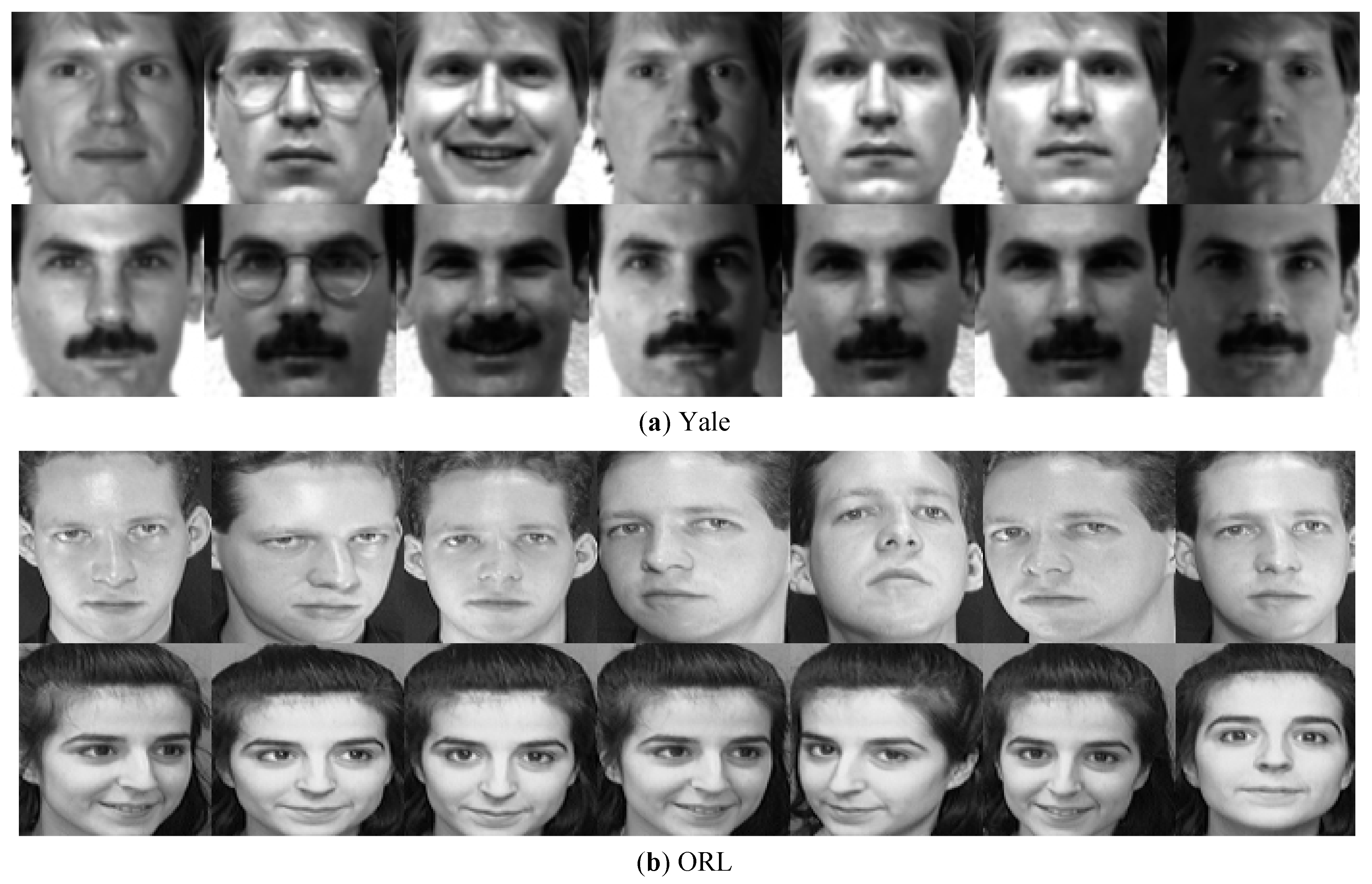
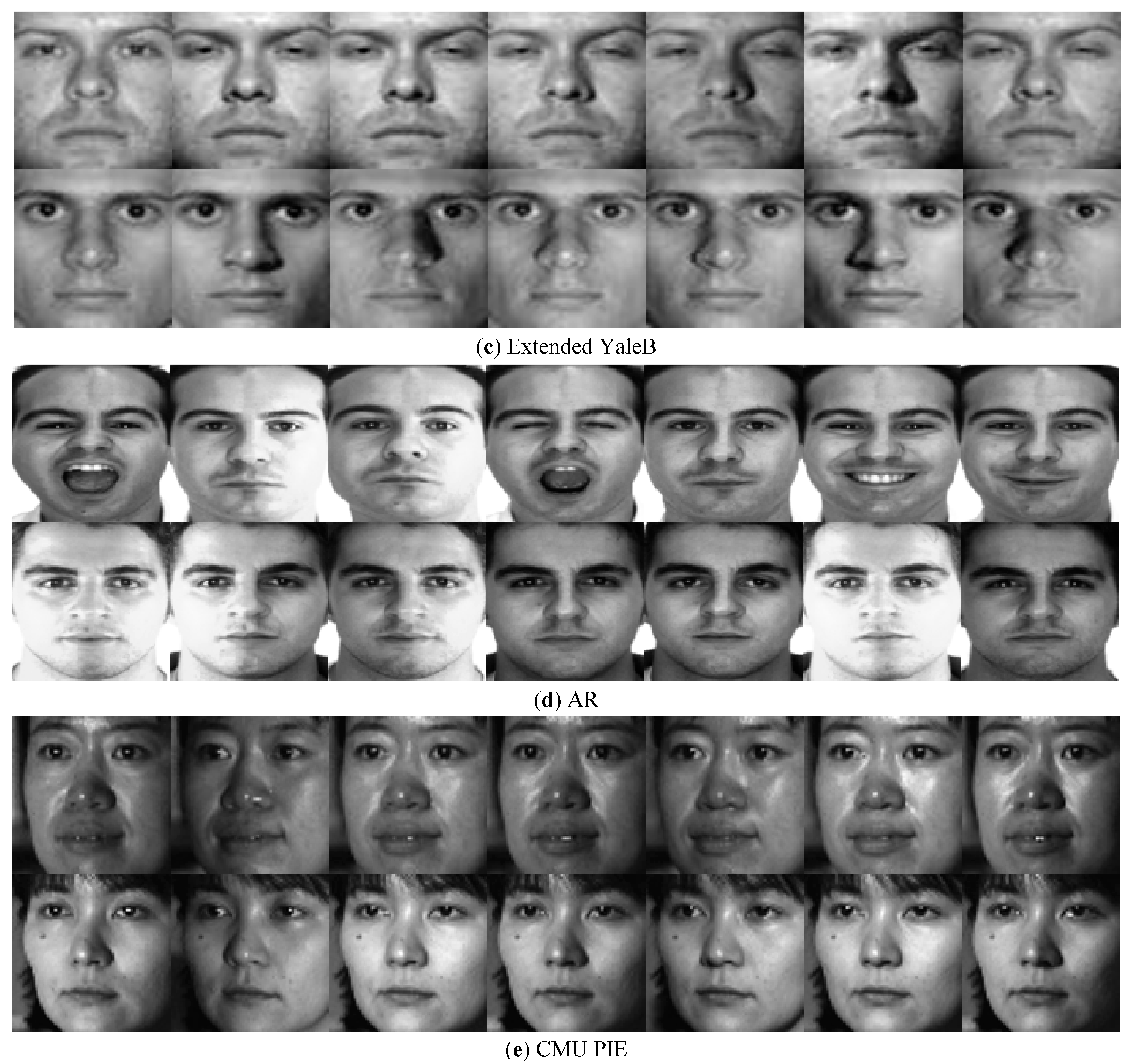
To evaluate the performance of the proposed SSRR-AGLP for classification, we test it on five facial image databases (Yale [52], ORL [53], Extended YaleB [54], AR [55] and CMU PIE [56]). The detailed information of the five databases utilized in our experiments is shown in Table 1 and some sample images from them are displayed in Figure 2. In all experiments, 50% samples of each subject are selected randomly for training and the remaining samples are used for testing in each database. Specifically, a part of the samples is randomly selected as labeled data in each training set, and the numbers of selected training and testing sets for experiments are shown in Table 2.
Moreover, to justify the superiority of the proposed SSRR-AGLP, we compare it with some well-known algorithms, such as traditional k-nearest neighbor (KNN) [57], least squares regression (LSR) [1], ridge regression (RR) [22], inter-class sparsity based discriminative least square regression (ICS_DLSR) [18] and the locality-constrained and label embedding dictionary learning (LCLE-DL) [35].

4.1. Parameter Setting

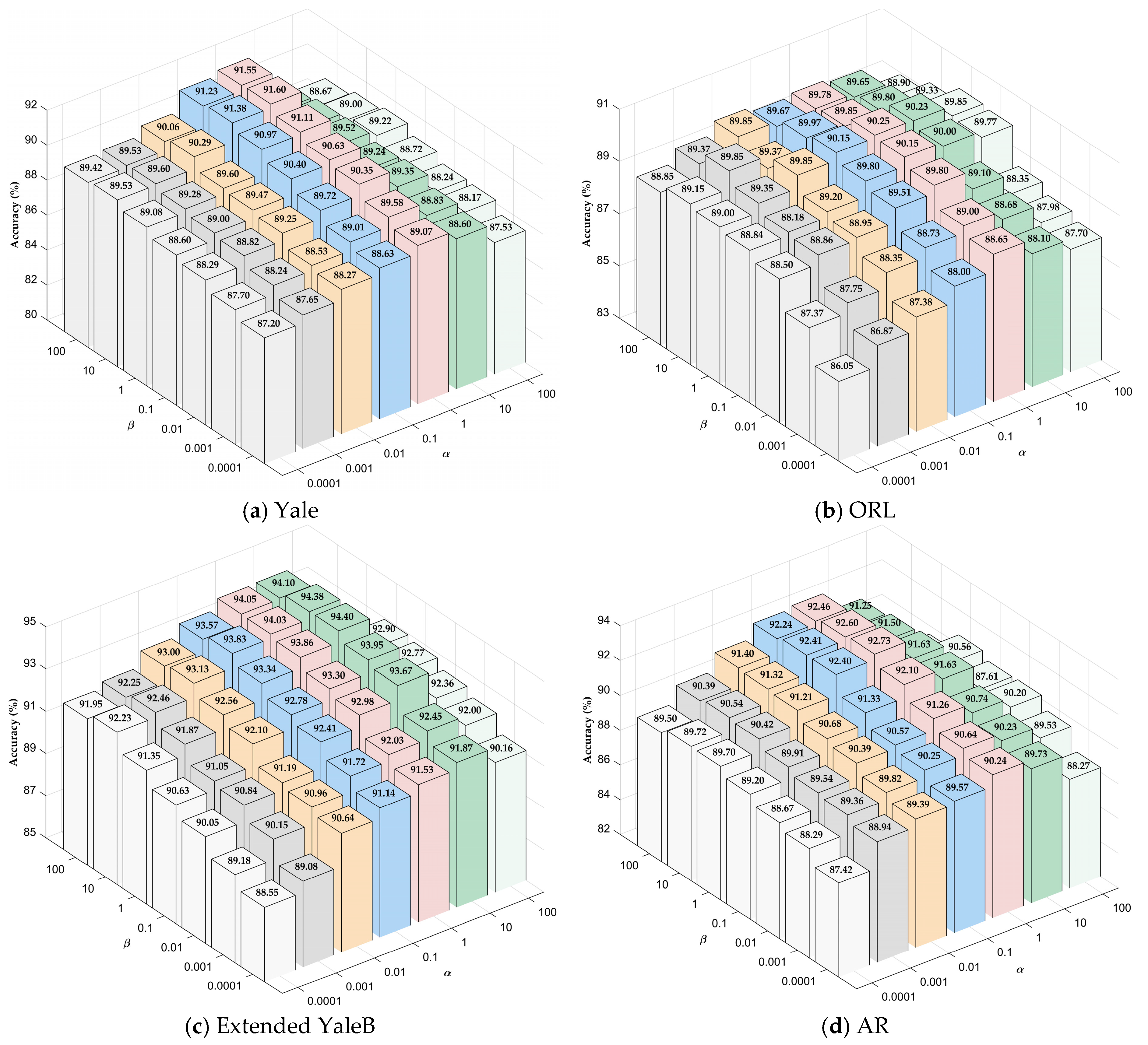
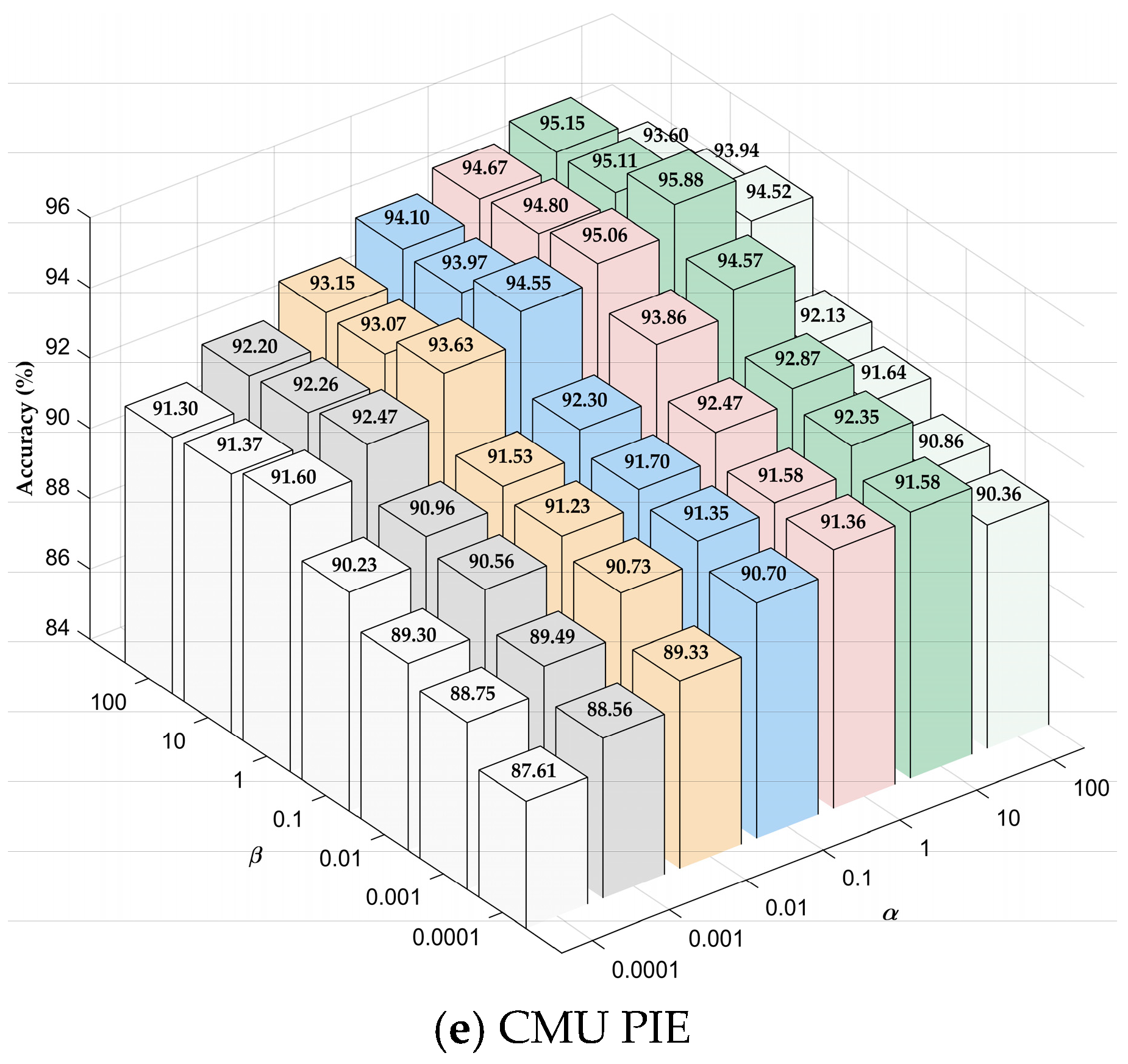
According to Section 3, there are three parameters, i.e., α, β and γ, that need to be determined in the objective function of the proposed SSRR-AGLP. The best values of these parameters are tuned by searching the grid {0.0001, 0.001, 0.01, 0.1, 1, 10, and 100} in an alternate manner. We first fix parameter γ as 0.01, and the influences of the parameters α and β on different datasets are illustrated in Figure 3. From these results, the tendencies of α and β on the accuracy rates increase first and then decrease for all the databases, which indicates that locality constraint term and label propagation can improve the performance of SSRR-AGLP. Moreover, when the values of parameters are set between 1 and 10, the performance of our SSRR-AGLP is insensitive to the parameter values. Then, we fix parameters α and β with best values, and the results of our algorithm under various values of parameter γ on the different databases are listed in Table 3. From this table, we can find the proposed SSRR-AGLP reaches the best performance when the parameter γ is set as 0.01 for all the databases. Moreover, when the parameters are set between 0.001 and 0.1, the performance of our SSRR-AGLP is insensitive to the parameter value of γ. Finally, we can find the best parameter values for our model are {α = 1, β = 10 and γ = 0.01} on Yale database, {α = 1, β = 1 and γ = 0.01} on ORL database, {α = 10, β = 1 and γ = 0.01} on Extended YaleB database, {α = 1, β = 1 and γ = 0.01} on AR database and {α = 10, β = 1 and γ = 0.01} on CMU PIE database. Therefore, according to the experimental results, we can set the parameters α and β as relatively larger values (1 and 10), and set the parameter γ as a small value (from 0.001 to 0.1) for the application tasks.

4.2. Experimental Results and Analysis

To fairly compare the performances of our approach and other algorithms, the average accuracy rates and standard deviations over 10 random training sample selection procedures of different algorithms are listed in Table 4. From Table 4, we can get the following observations: (1) KNN is sensitive to noise; its accuracy rate is lower than other methods. (2) The performance of RR is better than that of LSR, which indicates that RR can avoid the over-fitting problem effectively. (3) The accuracy rate of ICS_DLSR is higher than that of LSR and RR. This is because that the inter-class sparsity regularization term can improve discriminative ability of transformation matrix adequately. (4) By exploring the locality structure of the learned dictionary, the performance of LCLE_DL is better than that of RR and ICS_DLSR in most cases, which implies that the locality of data can improve the performance effectively. (5) The performance of the proposed SSRR-AGLP is consistently superior to other algorithms for five face image databases. It is because SSRR-AGLP not only employs both the labeled and unlabeled data to train the classifiers, but also takes advantage of the locality and sparsity of data for adaptive graph construction.
In the second experiment, to verify the performances of the proposed SSRR-AGLP under different numbers of labeled samples, we select 50% samples as the training set for each facial database, in which different numbers of samples are selected as labeled samples for each training set. Table 5 lists the best average accuracy rates obtained by SSRR-AGLP with varied numbers of labeled samples. We can see that with the increase in labeled samples, the performance of the proposed SSRR-AGLP is improved gradually.
In the third experiment, the predicted labels of SSRR-AGLP are compared with the traditional label propagation algorithms to evaluate the performance of SSRR-AGLP. Specifically, the number of the selected label samples for each database is set as the same as in the first experiment, and the accuracy of the predicted labels by SSRR-AGLP and LP is listed in Table 6. It can be seen that the performance of SSRR-AGLP is superior to that of LP due to the cooperation of adaptive graph leaning and label propagation in it. In other words, compared with the traditional LP which predicts the labels by constructing a graph in advance, adaptive graph learning in SSRR-AGLP can improve the predicted performance of SSRR-AGLP. Besides, according to the predicted labels of traditional LP algorithm, we utilize the ridge regression (RR) algorithm (denoted as LP + RR) for classification and the results for the five databases are listed Table 7. From Table 7, we can see that the performance of LP + RR is better than that of the RR algorithm, but still worse than that of SSRR-AGLP. This indicates that combining both of the LP and RR algorithms into a uniform framework can provide a benefit for classification tasks.
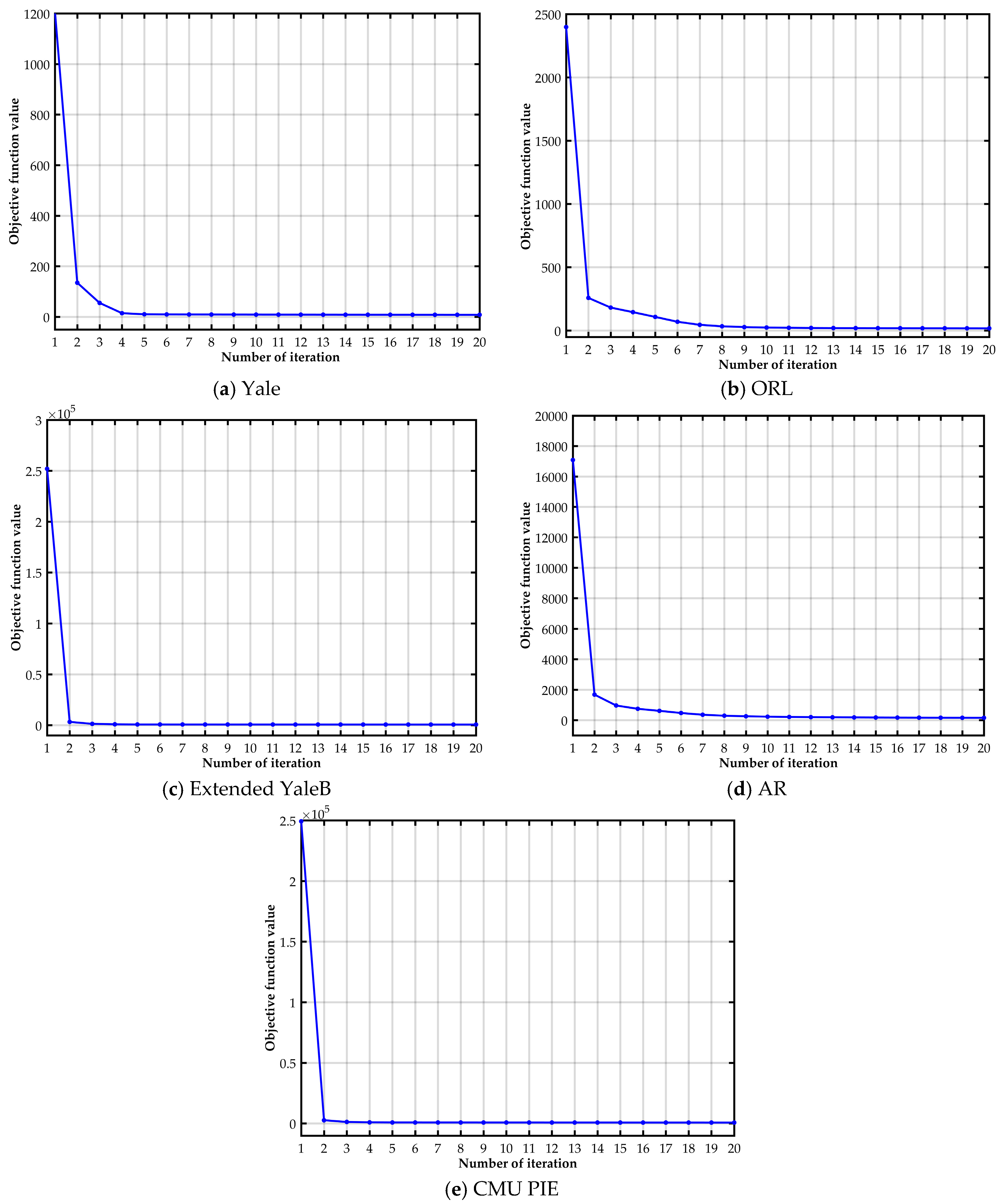
Finally, Figure 4 displays the convergence curves of SSRR-AGLP for five facial image databases. In this figure, the x-axis and y-axis denote the number of iterations and the value of the objective function, respectively. We can see that the proposed iterative updating algorithm converges very fast (usually within 20 iterations).

5. Conclusions

In this paper, we present a semi-supervised ridge regression algorithm which combines ridge regression with graph learning and label propagation into a unified framework. Compared with other approaches, the proposed SSRR-AGLP not only can adaptively construct graph based on the locality and sparsity of data, but also overcome the “out-of-sample” problem. Moreover, we design an effective iterative updating algorithm to solve the proposed framework and the convergence analysis is also provided accordingly. Extensive experiments indicate the effectiveness and superiority of the proposed SSRR-AGLP.
From the experimental results, the performance of the proposed SSRR-AGLP is affected by the parameter values. Therefore, how to extend our framework to a parameter-free approach is one focus in our future research. Furthermore, we only take one distance measurement, i.e., the exponential function in Equation (9), to characterize the local information of input data in this study. Hence, introducing more distance measurements (such as Euclidean distance, inner-product and so on) into our SSRR-AGLP so that the local geometrical structure of data can be better exploited is also future work.

Author Contributions

Data curation, X.G., C.C. and W.W.; Formal analysis, X.G., G.L. and W.W.; Methodology, Y.Y., J.D. and Y.C.; Writing—original draft, Y.Y., Y.C. and J.D.; Writing—review & editing, Y.Y. and Y.C.

Funding

This research was funded by the National Natural Science Foundation of China, grant numbers [61602221, 61806126 and 61762050], the Natural Science Foundation of Jiangxi Province, grant number [20171BAB21009], the Science and Technology Research Project of Jiangxi Provincial Department of Education grant numbers [GJJ160333, GJJ170234 and GJJ160315], the Project of Shandong Province Higher Educational Science and Technology Program, grant number [J16LN68], the Shandong Province Natural Science Foundation, grant number [ZR2017QF011], the Weifang Science and Technology Development Plan Project, grant numbers [2017GX006, 2018GX009], and the Jiangxi Province Graduate Innovation Project, grant numbers [YC2018-S175].

Conflicts of Interest

The authors declare no conflict of interest.

References

  1. Strutz, T. Data Fitting and Uncertainty: A Practical Introduction to Weighted Least Squares and Beyond; Vieweg: Wiesbaden, Germany, 2010. [Google Scholar]
  2. Krishnan, A.; Williams, L.J.; McIntosh, A.R.; Abdi, H. Partial Least Squares (PLS) methods for neuroimaging: A tutorial and review. Neuroimage 2011, 56, 455–475. [Google Scholar] [CrossRef] [PubMed]
  3. Ruppert, D.; Sheather, S.J.; Wand, M.P. An effective bandwidth selector for local least squares regression. J. Am. Statist. Assoc. 1995, 90, 1257–1270. [Google Scholar] [CrossRef]
  4. Gao, J.; Shi, D.; Liu, X. Significant vector learning to construct sparse kernel regression models. Neural Netw. 2007, 20, 791–798. [Google Scholar] [CrossRef] [PubMed]
  5. Gold, C.; Sollich, P. Model selection for support vector machine classification. Neurocomputing 2003, 55, 221–249. [Google Scholar] [CrossRef] [Green Version]
  6. Kim, H.; Park, H. Nonnegative matrix factorization based on alternating nonnegativity constrained least squares and active set method. SIAM J. Matrix Anal. Appl. 2008, 30, 713–730. [Google Scholar] [CrossRef]
  7. Li, Y.; Ngom, A. Nonnegative least-squares methods for the classification of high-dimensional biological data. IEEE/ACM Trans. Comput. Biol. Bioinform. (TCBB) 2013, 10, 447–456. [Google Scholar] [CrossRef] [PubMed]
  8. Wang, L.; Pan, C. Groupwise retargeted least-squares regression. IEEE Trans. Neural Netw. Learn. Syst. 2018, 29, 1352–1358. [Google Scholar] [CrossRef]
  9. Zhang, L.; Valaee, S.; Xu, Y.; Vedadi, F. Graph-based semi-supervised learning for indoor localization using crowdsourced data. Appl. Sci. 2017, 7, 467. [Google Scholar] [CrossRef]
  10. Zhang, Z.; Lai, Z.; Xu, Y.; Shao, L.; Wu, J.; Xie, G.S. Discriminative elastic-net regularized linear regression. IEEE Trans. Image Process. 2017, 26, 1466–1481. [Google Scholar] [CrossRef]
  11. Peng, Y.; Kong, W.; Yang, B. Orthogonal extreme learning machine for image classification. Neurocomputing 2017, 266, 458–464. [Google Scholar] [CrossRef]
  12. Yuan, H.; Zheng, J.; Lai, L.L.; Tang, Y.Y. A constrained least squares regression model. Inf. Sci. 2018, 429, 247–259. [Google Scholar] [CrossRef]
  13. Yuan, H.; Zheng, J.; Lai, L.L.; Tang, Y.Y. Semi-supervised graph-based retargeted least squares regression. Signal Proces. 2018, 142, 188–193. [Google Scholar] [CrossRef]
  14. Ruppert, D.; Wand, M.P. Multivariate locally weighted least squares regression. Ann. Stat. 1994, 22, 1346–1370. [Google Scholar] [CrossRef]
  15. Xiang, S.; Nie, F.; Meng, G.; Pan, C.; Zhang, C. Discriminative least squares regression for multiclass classification and feature selection. IEEE Trans. Neural Netw. Learn. Syst. 2012, 23, 1738–1754. [Google Scholar] [CrossRef] [PubMed]
  16. Zhang, X.Y.; Wang, L.; Xiang, S.; Liu, C.L. Retargeted least squares regression algorithm. IEEE Trans. Neural Netw. Learn. Syst. 2015, 26, 2206–2213. [Google Scholar] [CrossRef] [PubMed]
  17. De la Torre, F. A least-squares framework for component analysis. IEEE Trans. Pattern Anal. Mach. Intell. 2012, 34, 1041–1055. [Google Scholar] [CrossRef]
  18. Wen, J.; Xu, Y.; Li, Z.; Ma, Z.; Xu, Y. Inter-class sparsity based discriminative least square regression. Neural Netw. 2018, 102, 36–47. [Google Scholar] [CrossRef]
  19. Jolliffe, I. Principal Component Analysis, International Encyclopedia of Statistical Science; Springer: Berlin/Heidelberg, Germany, 2011; pp. 1094–1096. [Google Scholar]
  20. Bandos, T.V.; Bruzzone, L.; Camps-Valls, G. Classification of hyperspectral images with regularized linear discriminant analysis. IEEE Trans. Geosci. Remote Sens. 2009, 47, 862–873. [Google Scholar] [CrossRef]
  21. Lu, J.; Tan, Y.P. Regularized locality preserving projections and its extensions for face recognition. IEEE Trans. Syst. Man Cybern. Part B 2010, 40, 958–963. [Google Scholar]
  22. Brown, P.J.; Zidek, J.V. Adaptive multivariate ridge regression. Ann. Stat. 1980, 8, 64–74. [Google Scholar] [CrossRef]
  23. McDonald, G.C. Ridge regression. Wiley Interdiscip. Rev. Comput. Stat. 2009, 1, 93–100. [Google Scholar] [CrossRef]
  24. Işik, H.; Sezgin, E.; Avunduk, M.C. A new software program for pathological data analysis. Comput. Biol. Med. 2010, 40, 715–722. [Google Scholar] [CrossRef] [PubMed]
  25. Bashir, Y.; Aslam, A.; Kamran, M.; Qureshi, M.I.; Jahangir, A.; Rafiq, M.; Bibi, N.; Muhammad, N. On forgotten topological indices of some dendrimers structure. Molecules 2017, 22, 867. [Google Scholar] [CrossRef] [PubMed]
  26. Mahmood, Z.; Muhammad, N.; Bibi, N.; Ali, T. A review on state-of-the-art face recognition approaches. Fractals 2017, 25, 1750025. [Google Scholar] [CrossRef]
  27. Muhammad, N.; Bibi, N.; Qasim, I.; Jahangir, A.; Mahmood, Z. Digital watermarking using Hall property image decomposition method. Pattern Anal. Appl. 2018, 21, 997–1012. [Google Scholar] [CrossRef]
  28. Muhammad, N.; Bibi, N.; Wahab, A.; Mahmood, Z.; Akram, T.; Naqvi, S.; Sook, H.; Kim, D.-G. RImage de-noising with subband replacement and fusion process using bayes estimators. Comput. Electron. Eng. 2018, 70, 413–427. [Google Scholar] [CrossRef]
  29. Saunders, C.; Gammerman, A.; Vovk, V. Ridge Regression Learning Algorithm in Dual Variables; University of London: London, UK, 1998. [Google Scholar]
  30. Xue, H.; Zhu, Y.; Chen, S. Local ridge regression for face recognition. Neurocomputing 2009, 72, 1342–1346. [Google Scholar] [CrossRef] [Green Version]
  31. Huang, G.B.; Zhou, H.; Ding, X.; Zhang, R. Extreme learning machine for regression and multiclass classification. IEEE Trans. Syst. Man Cybern. Part B 2012, 42, 513–529. [Google Scholar] [CrossRef]
  32. Zhang, Y.; Wainwright, M.J.; Duchi, J.C. Communication-efficient algorithms for statistical optimization. Adv. Neural Inf. Process. Syst. 2012, 1502–1510. [Google Scholar] [CrossRef]
  33. An, S.; Liu, W.; Venkatesh, S. Face recognition using kernel ridge regression. In Proceedings of the IEEE Conference on Computer Vision and Pattern Recognition, Minneapolis, MN, USA, 17–22 June 2007; pp. 1–7. [Google Scholar]
  34. Liu, E.; Song, Y.; Liang, J. An accelerator for kernel ridge regression algorithms based on data partition. J. Univ. Sci. Technol. China 2018, 48, 284–289. [Google Scholar]
  35. Li, Z.; Lai, Z.; Xu, Y.; Zhang, D. A locality-constrained and label embedding dictionary learning algorithm for image classification. IEEE Trans. Neural Netw. Learn. Syst. 2017, 28, 278–293. [Google Scholar] [CrossRef] [PubMed]
  36. Yi, Y.; Shi, Y.; Zhang, H.; Wang, J.; Kong, J. Label propagation based semi-supervised non-negative matrix factorization for feature extraction. Neurocomputing 2015, 149, 1021–1037. [Google Scholar] [CrossRef]
  37. Yi, Y.; Bi, C.; Li, X.; Wang, J.; Kong, J. Semi-supervised local ridge regression for local matching based face recognition. Neurocomputing 2015, 167, 132–146. [Google Scholar] [CrossRef]
  38. Yi, Y.; Qiao, S.; Zhou, W.; Zheng, C.; Liu, Q.; Wang, J. Adaptive multiple graph regularized semi-supervised extreme learning machine. Soft Comput. 2018, 22, 3545–3562. [Google Scholar] [CrossRef]
  39. Rwebangira, M.R.; Lafferty, J. Local Linear Semi-Supervised Regression; School of Computer Science Carnegie Mellon University: Pittsburgh, PA, USA, 2009; p. 15213. [Google Scholar]
  40. Chang, X.; Lin, S.B.; Zhou, D.X. Distributed semi-supervised learning with kernel ridge regression. J. Mach. Learn. Res. 2017, 18, 1–22. [Google Scholar]
  41. Zhu, X.; Ghahramani, Z. Learning from Labeled and Unlabeled Data with Label Propagation. 2002. Available online: http://citeseerx.ist.psu.edu/viewdoc/download?doi=10.1.1.14.3864&rep=rep1&type=pdf (accessed on 14 December 2018).
  42. Wang, F.; Zhang, C. Label propagation through linear neighborhoods. IEEE Trans. Knowl. Data Eng. 2008, 20, 55–67. [Google Scholar] [CrossRef]
  43. Zhu, X.; Ghahramani, Z.; Lafferty, J.D. Semi-supervised learning using gaussian fields and harmonic functions. In Proceedings of the 20th International conference on Machine learning (ICML-03), Washington, DC, USA, 21–24 August 2003; pp. 912–919. [Google Scholar]
  44. Zhou, D.; Bousquet, O.; Lal, T.N.; Weston, J.; Schölkopf, B. Learning with local and global consistency. Adv. Neural Inf. Process. Syst. 2004, 321–328. [Google Scholar] [CrossRef]
  45. Qiao, L.; Zhang, L.; Chen, S.; Shen, D. Data-driven Graph Construction and Graph Learning: A. Review. Neurocomputing 2018, 312, 336–351. [Google Scholar] [CrossRef]
  46. Cheng, B.; Yang, J.; Yan, S.; Fu, Y.; Huang, TS. Learning With l1-Graph for Image Analysis. IEEE Trans. Image Process. 2010, 19, 858–866. [Google Scholar] [CrossRef]
  47. Rohban, M.H.; Rabiee, H.R. Supervised neighborhood graph construction for semi-supervised classification. Pattern Recognit. 2012, 45, 1363–1372. [Google Scholar] [CrossRef]
  48. Wright, J.; Yang, A.Y.; Ganesh, A.; Sastry, S.S.; Ma, Y. Robust face recognition via sparse representation. IEEE Trans. Pattern Anal. Mach. Intell. 2009, 31, 210–227. [Google Scholar] [CrossRef] [PubMed]
  49. Zhang, Z.; Xu, Y.; Yang, J.; Li, X.; Zhang, D. A survey of sparse representation: Algorithms and applications. IEEE Access 2015, 3, 490–530. [Google Scholar] [CrossRef]
  50. Nasrabadi, N.M. Pattern recognition and machine learning. J. Electron. Imaging 2007, 16, 049901. [Google Scholar]
  51. Cai, D.; He, X.; Han, J.; Huang, T.S. Graph regularized nonnegative matrix factorization for data representation. IEEE Trans. Pattern Anal. Mach. Intell. 2011, 33, 1548–1560. [Google Scholar] [PubMed]
  52. Georghiades, A.; Belhumeur, P.; Kriegman, D. Yale Face Database. Center for Computational Vision and Control at Yale University. 1997, 2, p. 6. Available online: http://cvc.yale.edu/projects/yalefaces/yalefa (accessed on 10 December 2002).
  53. Samaria, F.S.; Harter, A.C. Parameterisation of a stochastic model for human face identification. In Proceedings of the Second IEEE Workshop on Applications of Computer Vision, Sarasota, FL, USA, 5–7 December 1994; pp. 138–142. [Google Scholar] [Green Version]
  54. Lee, K.C.; Ho, J.; Kriegman, D.J. Acquiring linear subspaces for face recognition under variable lighting. IEEE Trans. Pattern Anal. Mach. Intell. 2005, 5, 684–698. [Google Scholar]
  55. Martinez, A.M. The AR Face Database; CVC Technical Report24; The Ohio State University: Columbus, OH, USA, 1998 June. [Google Scholar]
  56. Baker, S.; Bsat, M. The CMU Pose, Illumination, and Expression Database. IEEE Trans. Pattern Anal. Mach. Intell. 2003, 25, 1615. [Google Scholar]
  57. Duda, R.O.; Hart, P.E.; Stork, D.G. Pattern Classification; John Wiley & Sons: New York, NY, USA, 2012. [Google Scholar]
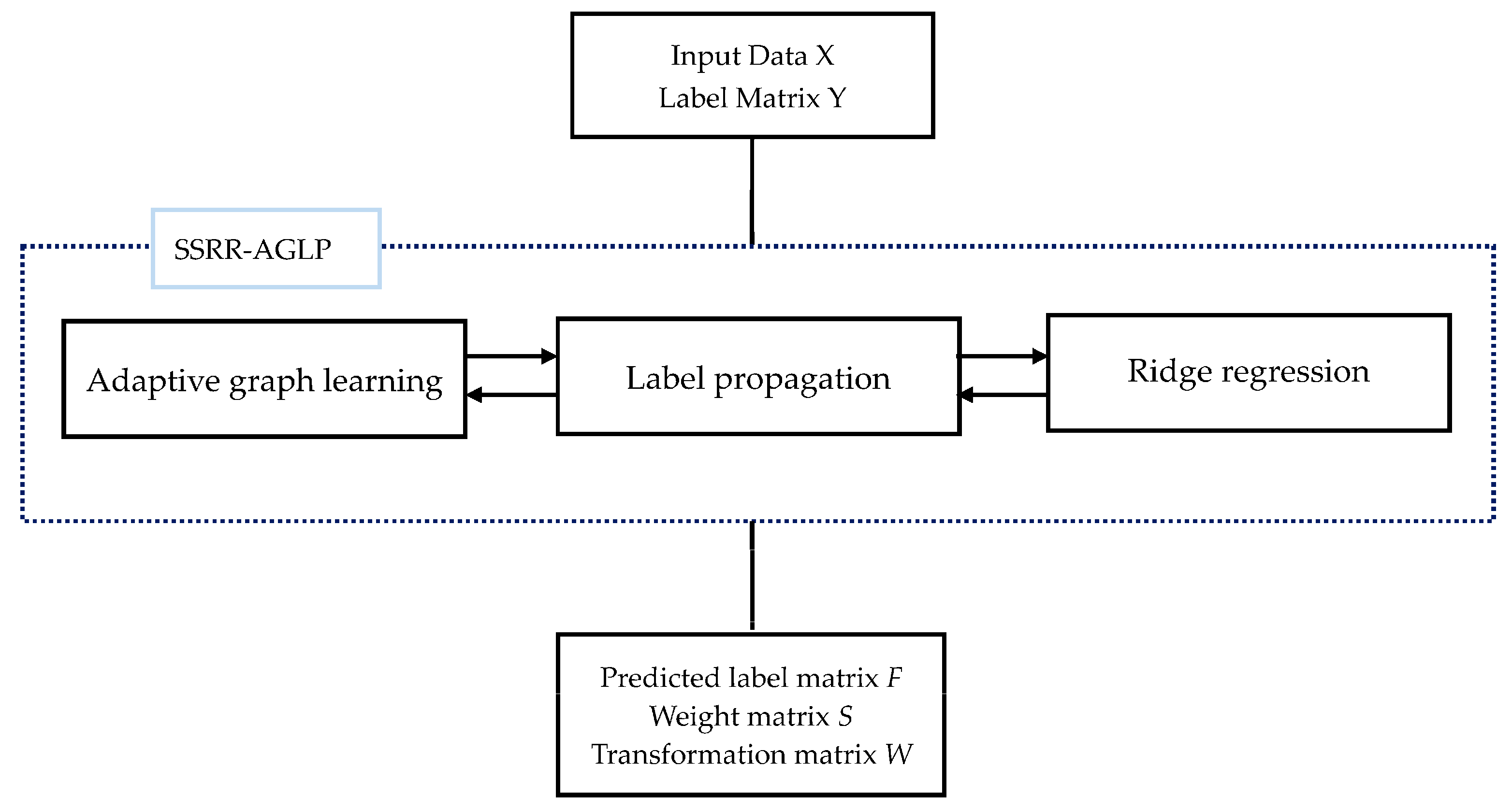
Figure 1. The flowchart of the proposed approach.
Applsci 08 02636 g001
Figure 2. Some of the images from five databases.
Applsci 08 02636 g002aApplsci 08 02636 g002b
Figure 3. The influence of the parameters on different databases.
Applsci 08 02636 g003aApplsci 08 02636 g003b
Figure 4. Convergence curves of objective function for different databases.
Applsci 08 02636 g004
Table 1. Detailed information of databases.
DatabaseSizeSamplesClassesPer Class
Yale32 × 321651511
ORL32 × 324004010
Extended YaleB32 × 3224323864
AR32 × 32140010014
CMU PIE32 × 3216326824
Table 2. Detailed information of sample selection for different databases.
DatabaseTraining Sample SizeTest Sample Size
Labeled SamplesUnlabeled Samples
Yale335
ORL325
Extended YaleB181432
AR437
CMU PIE6612
Table 3. The average accuracy (%) and standard deviation (%) of different values of parameter γ for different databases.
DatabaseYaleORLExtended YaleBARCMU PIE
γ = 0.000189.61 ± 5.2088.73 ± 4.6892.08 ± 5.6991.00 ± 4.3992.96 ± 3.57
γ = 0.00191.27 ± 5.7990.00 ± 3.1694.22 ± 6.7292.66 ± 5.4595.51 ± 3.41
γ = 0.0191.60 ± 5.8390.25 ± 3.7594.40 ± 6.8792.73 ± 5.0695.88 ± 3.55
γ = 0.191.00 ± 4.8089.95 ± 3.1894.24 ± 5.1891.93 ± 4.8695.37 + 3.87
γ = 190.52 ± 4.6988.76 ± 3.8793.13 ± 5.6091.00 ± 4.2494.19 + 3.46
γ = 1089.87 ± 5.6487.54 ± 3.2592.16 ± 5.0990.54 ± 3.6993.27 ± 3.23
γ = 10088.76 ± 5.7886.90 ± 3.6391.40 ± 4.2889.79 ± 4.5092.35 ± 3.08
Table 4. The average accuracy (%) and standard deviation (%) of different methods for different databases.
MethodYaleORLExtended YaleBARCMU PIE
KNN84.93 ± 7.2073.05 ± 2.6875.42 ± 6.9869.04 ± 6.9390.07 ± 6.51
LSR88.27 ± 7.9784.75 ± 1.6087.51 ± 7.2282.66 ± 6.7091.57 ± 5.41
RR89.07 ± 7.8285.75 ± 2.3088.33 ± 9.2386.77 ± 4.7292.44 ± 5.03
ICS_DLSR90.00 ± 2.4587.60 ± 1.9892.04 ± 0.8190.93 ± 1.4492.71 + 0.75
LCLE_DL90.40 ± 3.0087.65 ± 3.1191.93 ± 0.6290.91 ± 1.1493.91 + 1.34
SSRR-AGLP91.60 ± 5.8390.25 ± 3.7594.40 ± 6.8792.73 ± 5.0695.88 ± 3.55
Table 5. The average results of the proposed SSRR-AGLP with different numbers of labeled samples for five facial image databases.
DatabaseAccuracy (%)
Yale88.80 ± 5.56(2/4)91.60 ± 5.83(3/3)95.20 ± 4.88(4/2)
ORL83.25±2.92(2/3)90.25 ± 3.75(3/2)92.35 ± 2.16(4/1)
Extended YaleB92.07 ± 4.20(12/20)92.38 ± 4.23(16/16)94.40 ± 6.87(18/14)
AR90.37 ± 8.07(3/4)92.73 ± 5.06(4/3)94.27 ± 4.93(5/2)
CMU PIE85.78 ± 7.95(4/8)95.88 ± 3.55(6/6)93.82 ± 4.58(8/4)
Note that the two numbers in parentheses are the corresponding the quantities of labeled samples and unlabeled samples in training set.
Table 6. The label propagation accuracies (%) and standard deviations (%) of the proposed SSRR-AGLP and traditional LP for five facial image databases.
DatabaseLPSSRR-AGLP
Yale89.56 ± 5.8997.33 ± 2.30
ORL88.13 ± 2.3890.25 ± 3.81
Extended YaleB77.39 ± 8.3095.55 ± 5.15
AR78.00 ± 9.2797.63 ± 3.40
CMU PIE88.55 ± 9.7591.74 ± 6.83
Table 7. The average classification accuracies (%) and standard deviations (%) of RR, RR based on the predicted labels of traditional LP and SSRR-AGLP for five facial image databases.
DatabaseRRLP + RRSSRR-AGLP
Yale89.07 ± 7.8289.20 ± 6.8991.60 ± 5.83
ORL85.75 ± 2.3087.55 ± 2.3490.25 ± 3.75
Extended YaleB88.33 ± 9.2391.89 ± 7.8994.40 ± 6.87
AR86.77 ± 4.7288.44 ± 4.0792.73 ± 5.06
CMU PIE92.44 ± 5.0392.95 ± 5.1895.88 ± 3.55