A Measurement System for Time Constant of Thermocouple Sensor Based on High Temperature Furnace


Abstract
:1. Introduction
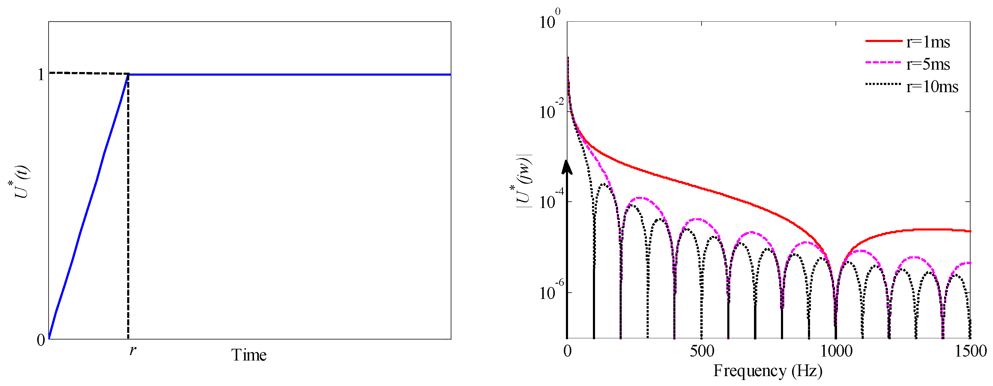
2. Analysis of Ramp Excitation Signal
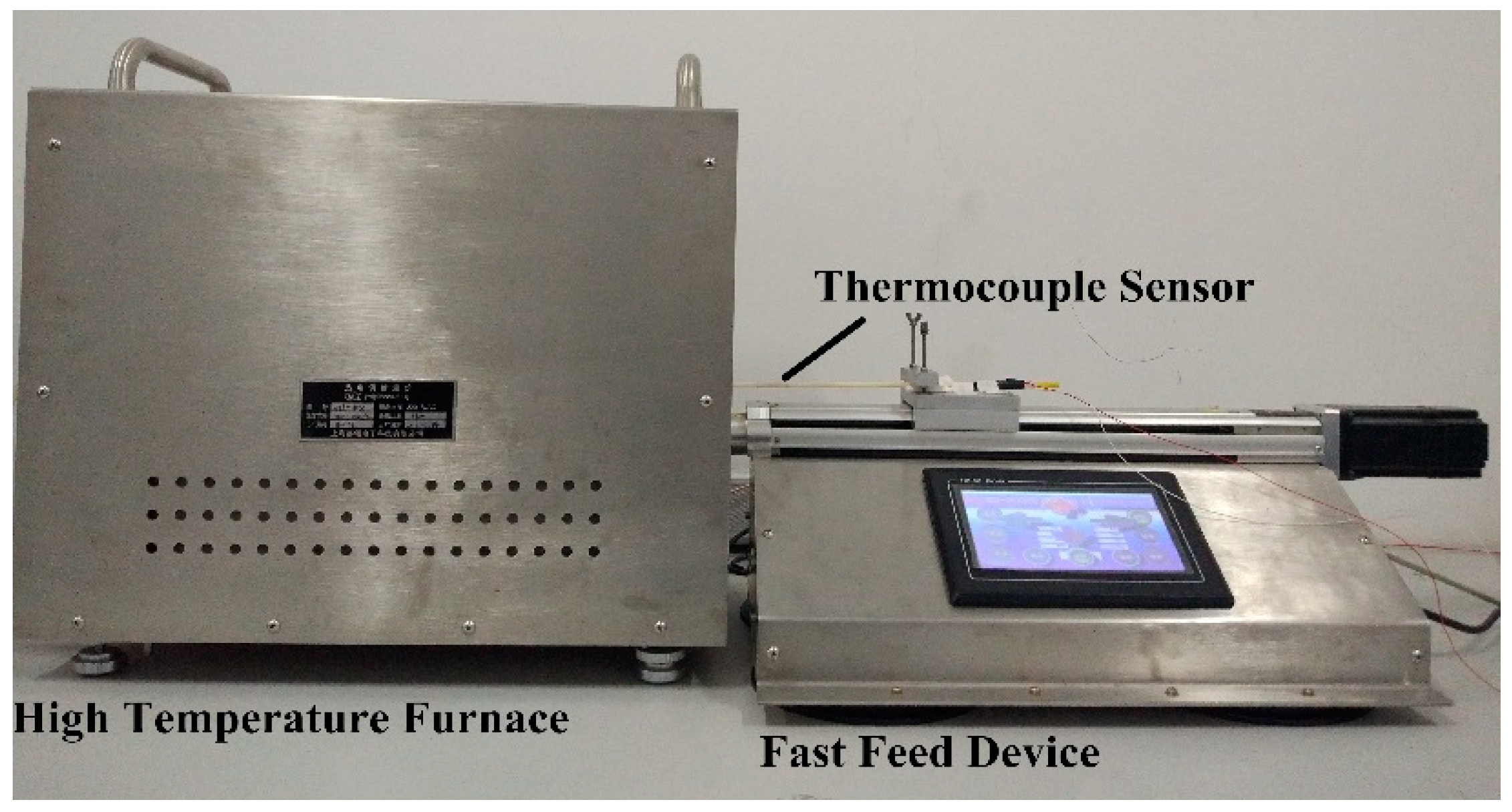
3. Measurement System for Time Constant Based on High Temperature Furnace
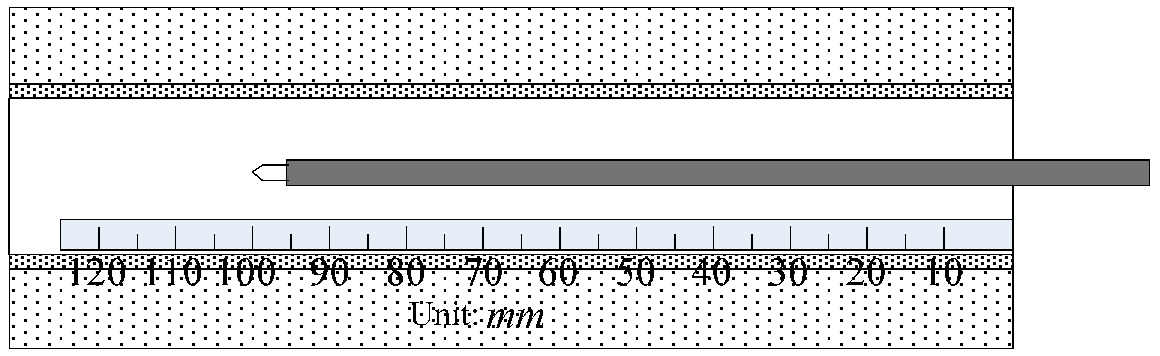
3.1. Generation of Ramp Temperature Excitation
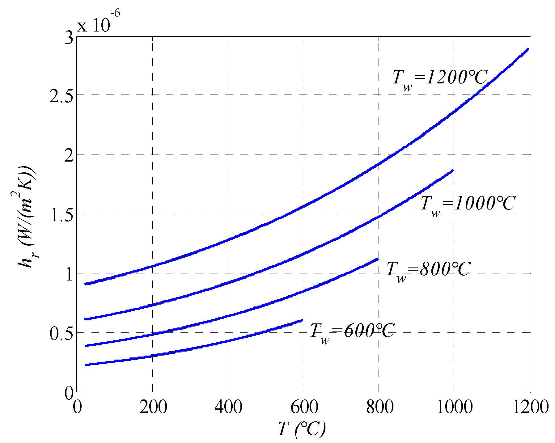
3.2. Analysis of Heat Transfer Environment in High Temperature Furnace
4. Experiment
4.1. Analysis of Type A Standard Uncertainty
4.2. Analysis of Type B Standard Uncertainty
4.3. Combined Standard Uncertainty and Expanded Uncertainty
5. Conclusions
Author Contributions
Funding
Conflicts of Interest
References
- Xiong, J.; Yu, H.Z. Response Delay of Thermal Sensors. J. Electron. Meas. Instrum. 2003, 17, 1–3. [Google Scholar]
- Wang, X.N.; Yu, F.Z.; Yang, S.J.; Qi, M.Y.; Ye, S.L. Study of TFTC Dynamic Character Based on Lumped Capacitance Method. Chin. J. Sens. Actuators 2014, 27, 1627–1631. [Google Scholar]
- Zhao, S.A.; Liao, L.; Chen, Y. 1700 °C Hot Wind Tunnel for Thermal Calibration. Metrol. Meas. Technol. 2000, 20, 3–6. [Google Scholar]
- Yang, Z.X.; Meng, X.F. Research on the Dynamic Calibration of Thermocouple and Temperature Excitation Signal Generation Method Based on Shock-Tube Theory. J. Eng. Gas Turb. Power 2014, 136, 071602. [Google Scholar] [CrossRef]
- Yang, Z.X.; Meng, X.F. Study on Transient Temperature Generator and Dynamic Compensation Technology. Appl. Mech. Mater. 2014, 2, 161–164. [Google Scholar] [CrossRef]
- Garinei, A.; Tagliaferri, E. A laser calibration system for in situ dynamic characterization of temperature sensors. Sens. Actuators A-Phys. 2013, 190, 19–24. [Google Scholar] [CrossRef]
- Serio, B.; Nika, P.; Prenel, J.P. Static and dynamic calibration of thin–film thermocouples by means of a laser modulation technique. Rev. Sci. Instrum. 2000, 71, 4306–4313. [Google Scholar] [CrossRef]
- Arwatz, G.; Bahri, C.; Smits, A.J.; Hultmark, M. Dynamic calibration and modeling of a cold wire for temperature measurement. Meas. Sci. Technol. 2013, 24, 125301. [Google Scholar] [CrossRef]
- Hao, X.J.; Li, K.J.; Liu, J.; Zhou, H.-C.; Huang, L. Traceability Dynamic Calibration of Temperature Sensor Based on CO2 Laser. Acta Armamentarii 2009, 30, 156–159. [Google Scholar]
- Feng, H.; Zhao, C.Y.; Xie, Y.N.; Wang, W.L.; Zhang, X.; Zhang, Z.J. Research on dynamic calibration and dynamic compensation of K-type thermocouple. In Proceedings of the 2014 IEEE International Instrumentation and Measurement Technology Conference (I2MTC) Proceedings, Montevideo, Uruguay, 12–15 May 2014; pp. 267–271. [Google Scholar]
- Castellini, P.; Rossi, G.L. Dynamic characterization of temperature sensors by laser excitation. Rev. Sci. Instrum. 1996, 67, 2595–2601. [Google Scholar] [CrossRef]
- Hashemian, H.M.; Jiang, J. Using the noise analysis technique to detect response time problems in the sensing lines of nuclear plant pressure transmitters. Prog. Nucl. Energy 2010, 52, 367–373. [Google Scholar] [CrossRef]
- Al-Dawery, S.K.; Alrahawi, A.M.; Al-Zobai, K.M. Dynamic modeling and control of plate heat exchanger. Int. J. Heat Mass Tran. 2009, 55, 6873–6880. [Google Scholar] [CrossRef]
- Tashiro, Y.; Biwa, T.; Yazaki, T. Calibration of a thermocouple for measurement of oscillating temperature. Rev. Sci. Instrum. 2005, 76, 124901. [Google Scholar] [CrossRef]
- Kim, S.J.; Park, G.C. Development of algorithm to measure temperatures of liquid/gas phases using micro-thermocouple and experiment with optical chopper. J. Mech. Sci. Technol. 2007, 21, 184–195. [Google Scholar] [CrossRef]
- Zhang, Z.J.; Li, Y.F. A dynamic calibration system of thermocouple sensor based on high temperature furnace. In Proceedings of the IEEE International Instrumentation and Measurement Technology Conference (I2MTC): Discovering New Horizons in Instrumentation and Measurement, Proceedings, Houston, TX, USA, 14–17 May 2018; pp. 1–5. [Google Scholar]


| Rise Time r (ms) | Rise Time r/Time Constant τ (%) | Estimate of Time Constant (ms) | Relative Error (%) |
|---|---|---|---|
| 20 | 2 | 1010 | 1.0 |
| 50 | 5 | 1025 | 2.5 |
| 100 | 10 | 1050 | 5.0 |
| 150 | 15 | 1075 | 7.5 |
| 200 | 20 | 1100 | 10 |
| n | Time Constant (s) | n | Time Constant (s) |
|---|---|---|---|
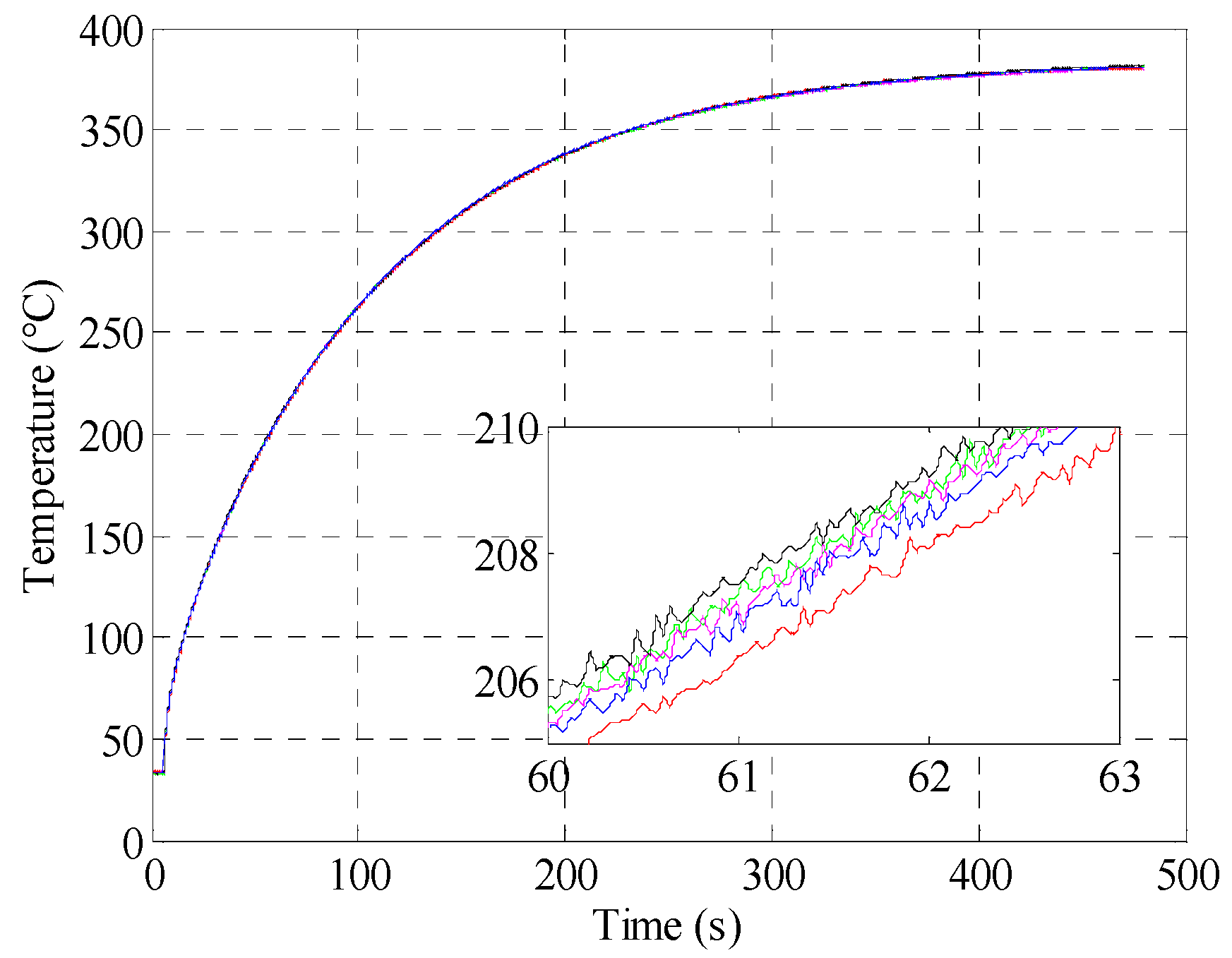
| 1 | 87.7232 | 4 | 87.2350 |
| 2 | 87.6740 | 5 | 87.9329 |
| 3 | 88.2180 |
| n | 2 | 3 | 4 | 5 | 6 | 7 | 8 | 9 |
|---|---|---|---|---|---|---|---|---|
| C | 1.13 | 1.69 | 2.06 | 2.33 | 2.53 | 2.70 | 2.85 | 2.97 |
| ν | 0.9 | 1.8 | 2.7 | 3.6 | 4.5 | 5.3 | 6.0 | 6.8 |
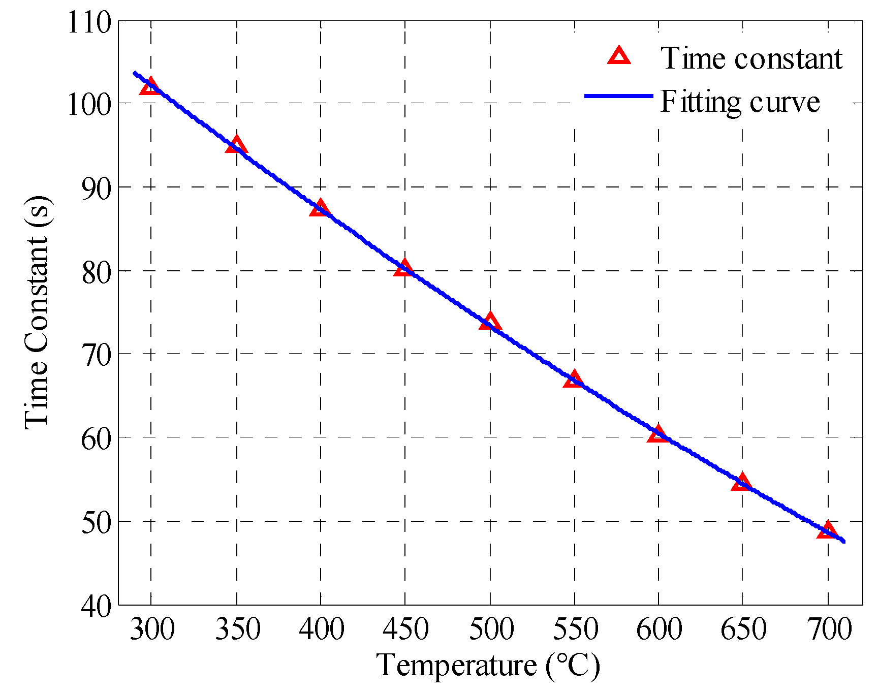
| Temperature (°C) | Time Constant (s) | Temperature (°C) | Time Constant (s) |
|---|---|---|---|
| 300 | 101.993 | 550 | 66.88 |
| 350 | 94.909 | 600 | 60.258 |
| 400 | 87.355 | 650 | 54.387 |
| 450 | 80.071 | 700 | 48.819 |
| 500 | 73.672 |
© 2018 by the authors. Licensee MDPI, Basel, Switzerland. This article is an open access article distributed under the terms and conditions of the Creative Commons Attribution (CC BY) license (http://creativecommons.org/licenses/by/4.0/).
Share and Cite
Li, Y.; Zhang, Z.; Hao, X.; Yin, W. A Measurement System for Time Constant of Thermocouple Sensor Based on High Temperature Furnace. Appl. Sci. 2018, 8, 2585. https://doi.org/10.3390/app8122585
Li Y, Zhang Z, Hao X, Yin W. A Measurement System for Time Constant of Thermocouple Sensor Based on High Temperature Furnace. Applied Sciences. 2018; 8(12):2585. https://doi.org/10.3390/app8122585
Chicago/Turabian StyleLi, Yanfeng, Zhijie Zhang, Xiaojian Hao, and Wuliang Yin. 2018. "A Measurement System for Time Constant of Thermocouple Sensor Based on High Temperature Furnace" Applied Sciences 8, no. 12: 2585. https://doi.org/10.3390/app8122585
APA StyleLi, Y., Zhang, Z., Hao, X., & Yin, W. (2018). A Measurement System for Time Constant of Thermocouple Sensor Based on High Temperature Furnace. Applied Sciences, 8(12), 2585. https://doi.org/10.3390/app8122585