Combination of High-Resolution Optical Coherence Tomography and Raman Spectroscopy for Improved Staging and Grading in Bladder Cancer


Abstract
Featured Application
Abstract
1. Introduction
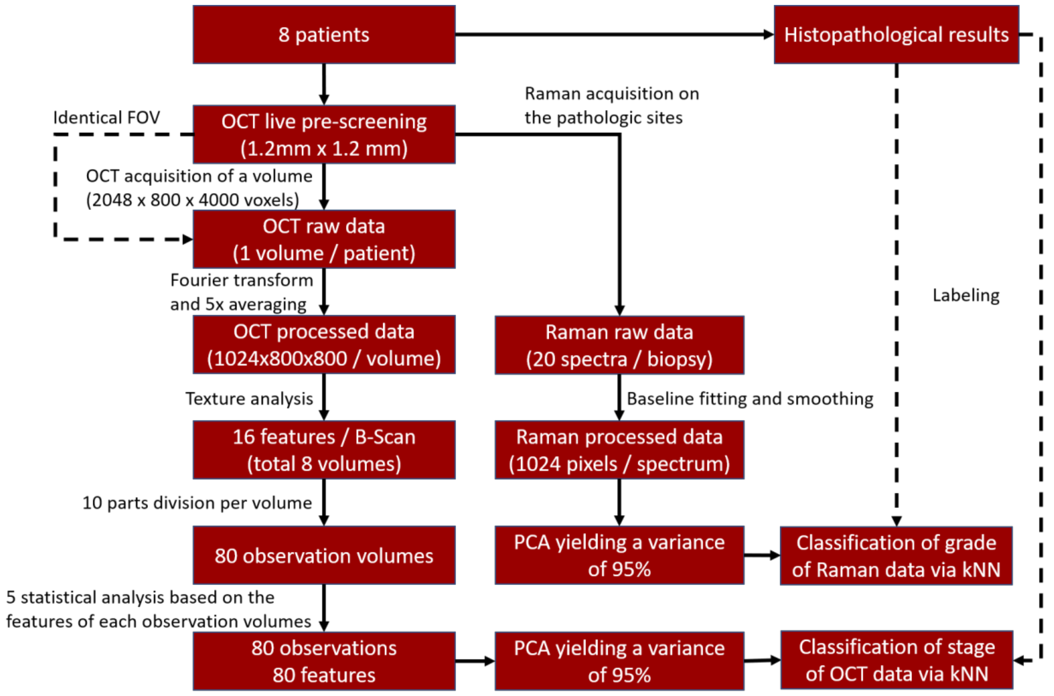
2. Materials and Methods
2.1. Patients
2.2. OCT System
2.3. RS System
2.4. OCT Texture Analysis
2.5. RS Analysis
2.6. Principal Component Analysis and Classifier Training
3. Results
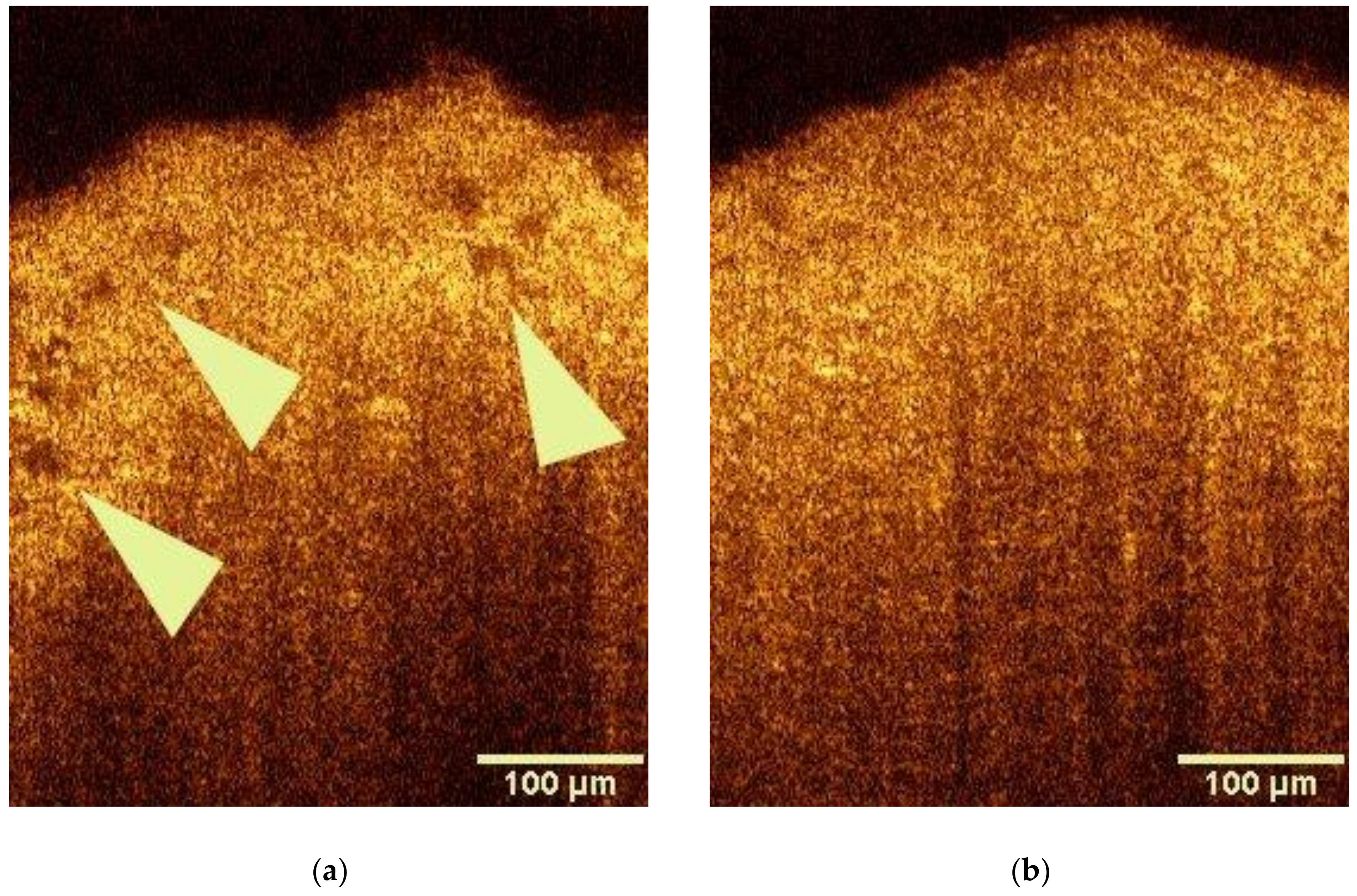
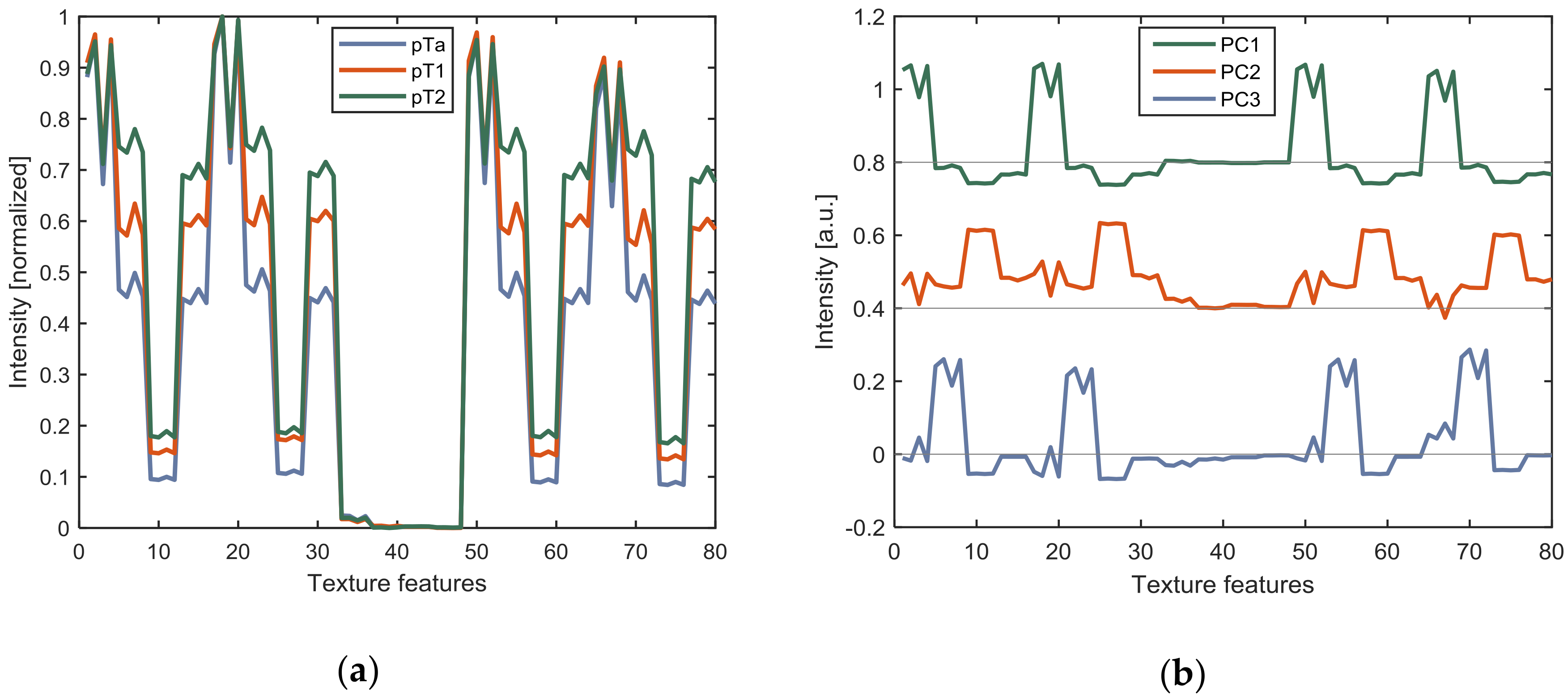
3.1. OCT Analysis
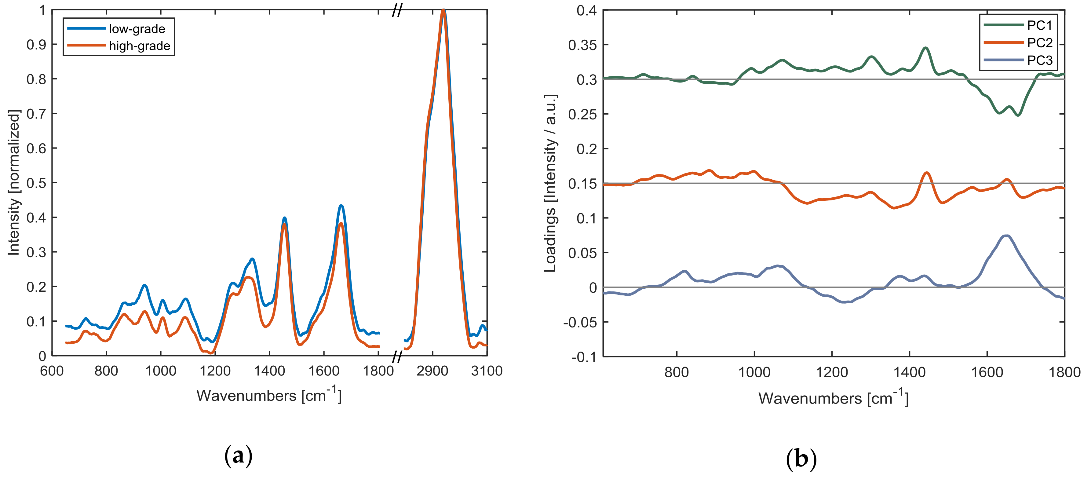
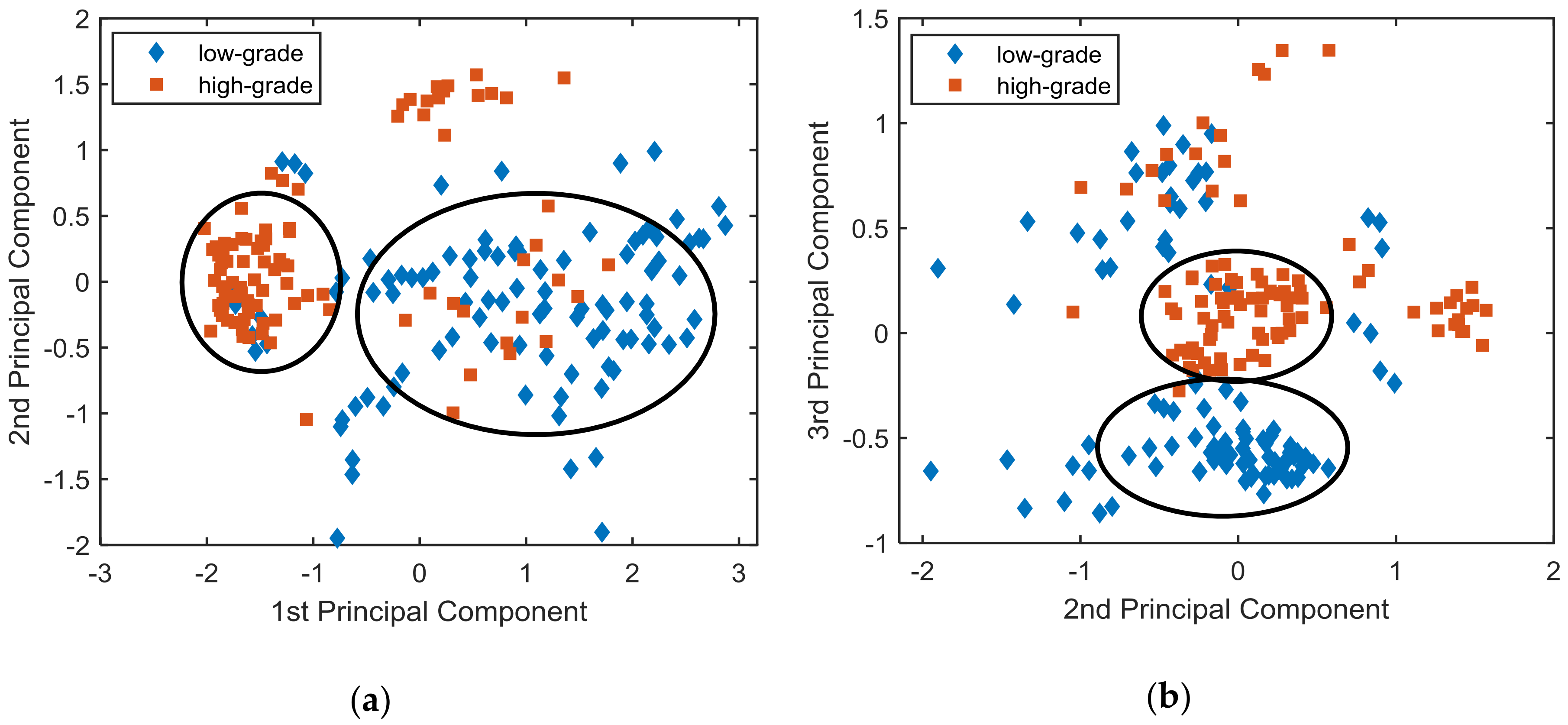
3.2. Raman Analysis
4. Discussion
5. Conclusions
Author Contributions
Funding
Acknowledgments
Conflicts of Interest
References
- Siegel, R.L.; Miller, K.D.; Jemal, A. Cancer statistics, 2018: Cancer Statistics, 2018. CA Cancer J. Clin. 2018, 68, 7–30. [Google Scholar] [CrossRef] [PubMed]
- Bray, F.; Ferlay, J.; Soerjomataram, I.; Siegel, R.L.; Torre, L.A.; Jemal, A. Global cancer statistics 2018: GLOBOCAN estimates of incidence and mortality worldwide for 36 cancers in 185 countries: Global Cancer Statistics 2018. CA Cancer J. Clin. 2018. [Google Scholar] [CrossRef] [PubMed]
- Antoni, S.; Ferlay, J.; Soerjomataram, I.; Znaor, A.; Jemal, A.; Bray, F. Bladder Cancer Incidence and Mortality: A Global Overview and Recent Trends. Eur. Urol. 2017, 71, 96–108. [Google Scholar] [CrossRef] [PubMed]
- Kerr, L.T.; Lynn, T.M.; Cullen, I.M.; Daly, P.J.; Shah, N.; O’Dea, S.; Malkin, A.; Hennelly, B.M. Methodologies for bladder cancer detection with Raman based urine cytology. Anal. Methods 2016, 8, 4991–5000. [Google Scholar] [CrossRef]
- Li, S.; Li, L.; Zeng, Q.; Zhang, Y.; Guo, Z.; Liu, Z.; Jin, M.; Su, C.; Lin, L.; Xu, J.; Liu, S. Characterization and noninvasive diagnosis of bladder cancer with serum surface enhanced Raman spectroscopy and genetic algorithms. Sci. Rep. 2015, 5. [Google Scholar] [CrossRef] [PubMed]
- Cauberg, E.C.C.; de Bruin, D.M.; Faber, D.J.; van Leeuwen, T.G.; de la Rosette, J.J.M.C.H.; de Reijke, T.M. A New Generation of Optical Diagnostics for Bladder Cancer: Technology, Diagnostic Accuracy, and Future Applications. Eur. Urol. 2009, 56, 287–297. [Google Scholar] [CrossRef] [PubMed]
- Kallaway, C.; Almond, L.M.; Barr, H.; Wood, J.; Hutchings, J.; Kendall, C.; Stone, N. Advances in the clinical application of Raman spectroscopy for cancer diagnostics. Photodiagn. Photodyn. Ther. 2013, 10, 207–219. [Google Scholar] [CrossRef] [PubMed]
- Lerner, S.P.; Goh, A. Novel endoscopic diagnosis for bladder cancer: Endoscopic Imaging for Bladder Cancer. Cancer 2015, 121, 169–178. [Google Scholar] [CrossRef] [PubMed]
- Fujimoto, J.G.; Pitris, C.; Boppart, S.A.; Brezinski, M.E. Optical Coherence Tomography: An Emerging Technology for Biomedical Imaging and Optical Biopsy. Neoplasia 2000, 2, 9–25. [Google Scholar] [CrossRef] [PubMed]
- Fercher, A.F.; Drexler, W.; Hitzenberger, C.K.; Lasser, T. Optical coherence tomography—Principles and applications. Rep. Prog. Phys. 2003, 66, 239. [Google Scholar] [CrossRef]
- Huang, D.; Swanson, E.; Lin, C.; Schuman, J.; Stinson, W.; Chang, W.; Hee, M.; Flotte, T.; Gregory, K.; Puliafito, C.; Fujimoto, J. Optical Coherence Tomography. Science 1991, 254, 1178–1181. [Google Scholar] [CrossRef] [PubMed]
- Van Manen, L.; Dijkstra, J.; Boccara, C.; Benoit, E.; Vahrmeijer, A.L.; Gora, M.J.; Mieog, J.S.D. The clinical usefulness of optical coherence tomography during cancer interventions. J. Cancer Res. Clin. Oncol. 2018. [Google Scholar] [CrossRef] [PubMed]
- Yuan, Z.; Wang, Z.; Pan, R.; Liu, J.; Cohen, H.; Pan, Y. High-resolution imaging diagnosis and staging of bladder cancer: Comparison between optical coherence tomography and high-frequency ultrasound. J. Biomed. Opt. 2008, 13, 054007. [Google Scholar] [CrossRef] [PubMed]
- Lerner, S.P.; Goh, A.C.; Tresser, N.J.; Shen, S.S. Optical Coherence Tomography as an Adjunct to White Light Cystoscopy for Intravesical Real-Time Imaging and Staging of Bladder Cancer. Urology 2008, 72, 133–137. [Google Scholar] [CrossRef] [PubMed]
- Schmidbauer, J.; Remzi, M.; Klatte, T.; Waldert, M.; Mauermann, J.; Susani, M.; Marberger, M. Fluorescence Cystoscopy with High-Resolution Optical Coherence Tomography Imaging as an Adjunct Reduces False-Positive Findings in the Diagnosis of Urothelial Carcinoma of the Bladder. Eur. Urol. 2009, 56, 914–919. [Google Scholar] [CrossRef] [PubMed]
- Gossage, K.W.; Tkaczyk, T.S.; Rodriguez, J.J.; Barton, J.K. Texture analysis of optical coherence tomography images: Feasibility for tissue classification. J. Biomed. Opt. 2003, 8, 570–575. [Google Scholar] [CrossRef] [PubMed]
- Bhattacharjee, M.; Ashok, P.C.; Rao, K.D.; Majumder, S.K.; Verma, Y.; Gupta, P.K. Binary tissue classification studies on resected human breat tissues using optical coherence tomography images. J. Innov. Opt. Health Sci. 2011, 04, 59–66. [Google Scholar] [CrossRef]
- Krafft, C.; Popp, J. The many facets of Raman spectroscopy for biomedical analysis. Anal. Bioanal. Chem. 2015, 407, 699–717. [Google Scholar] [CrossRef] [PubMed]
- Butler, H.J.; Ashton, L.; Bird, B.; Cinque, G.; Curtis, K.; Dorney, J.; Esmonde-White, K.; Fullwood, N.J.; Gardner, B.; Martin-Hirsch, P.L.; et al. Using Raman spectroscopy to characterize biological materials. Nat. Protoc. 2016, 11, 664–687. [Google Scholar] [CrossRef] [PubMed]
- Talari, A.C.S.; Movasaghi, Z.; Rehman, S.; Rehman, I. Raman Spectroscopy of Biological Tissues. Appl. Spectrosc. Rev. 2015, 50, 46–111. [Google Scholar] [CrossRef]
- Cordero, E.; Latka, I.; Matthäus, C.; Schie, I.W.; Popp, J. In-vivo Raman spectroscopy: From basics to applications. J. Biomed. Opt. 2018, 23, 1–23. [Google Scholar] [CrossRef] [PubMed]
- Ferraro, J.R.; Nakamoto, K.; Brown, C.W. Introductory Raman Spectroscopy, 2nd ed.; Academic Press: Amsterdam, The Netherlands; Boston, MA, USA, 2003; ISBN 978-0-12-254105-6. [Google Scholar]
- Movasaghi, Z.; Rehman, S.; Rehman, I.U. Raman Spectroscopy of Biological Tissues. Appl. Spectrosc. Rev. 2007, 42, 493–541. [Google Scholar] [CrossRef]
- Rehman, I.; Movasaghi, Z.; Rehman, S. Vibrational Spectroscopy for Tissue Analysis; Series in Medical Physics and Biomedical Engineering; CRC Press: Boca Raton, FL, USA, 2012; ISBN 978-1-4398-3608-8. [Google Scholar]
- De Jong, B.W.D.; Schut, T.B.; Wolffenbuttel, K.P.; Nijman, J.M.; Kok, D.J.; Puppels, G.J. Identification of bladder wall layers by Raman spectroscopy. J. Urol. 2002, 168, 1771–1778. [Google Scholar] [CrossRef]
- De Jong, B.W.D.; Bakker Schut, T.C.; Maquelin, K.; van der Kwast, T.; Bangma, C.H.; Kok, D.-J.; Puppels, G.J. Discrimination between Nontumor Bladder Tissue and Tumor by Raman Spectroscopy. Anal. Chem. 2006, 78, 7761–7769. [Google Scholar] [CrossRef] [PubMed]
- Crow, P.; Molckovsky, A.; Stone, N.; Uff, J.; Wilson, B.; WongKeeSong, L.-M. Assessment of fiberoptic near-infrared raman spectroscopy for diagnosis of bladder and prostate cancer. Urology 2005, 65, 1126–1130. [Google Scholar] [CrossRef] [PubMed]
- Stone, N.; Hart Prieto, M.C.; Crow, P.; Uff, J.; Ritchie, A.W. The use of Raman spectroscopy to provide an estimation of the gross biochemistry associated with urological pathologies. Anal. Bioanal. Chem. 2007, 387, 1657–1668. [Google Scholar] [CrossRef] [PubMed]
- Draga, R.O.P.; Grimbergen, M.C.M.; Vijverberg, P.L.M.; Swol, C.F.P.; van Jonges, T.G.N.; Kummer, J.A.; Ruud Bosch, J.L.H. In Vivo Bladder Cancer Diagnosis by High-Volume Raman Spectroscopy. Anal. Chem. 2010, 82, 5993–5999. [Google Scholar] [CrossRef] [PubMed]
- Schie, I.W.; Krafft, C.; Popp, J. Cell classification with low-resolution Raman spectroscopy (LRRS). J. Biophotonics 2016, 9, 994–1000. [Google Scholar] [CrossRef] [PubMed]
- Chen, H.; Li, X.; Broderick, N.; Liu, Y.; Zhou, Y.; Han, J.; Xu, W. Identification and characterization of bladder cancer by low-resolution fiber-optic Raman spectroscopy. J. Biophotonics 2018, e201800016. [Google Scholar] [CrossRef] [PubMed]
- Ashok, P.C.; Praveen, B.B.; Bellini, N.; Riches, A.; Dholakia, K.; Herrington, C.S. Multi-modal approach using Raman spectroscopy and optical coherence tomography for the discrimination of colonic adenocarcinoma from normal colon. Biomed. Opt. Express 2013, 4, 2179–2186. [Google Scholar] [CrossRef] [PubMed]
- Evans, J.W.; Zawadzki, R.J.; Liu, R.; Chan, J.W.; Lane, S.M.; Werner, J.S. Optical coherence tomography and Raman spectroscopy of the ex-vivo retina. J. Biophotonics 2009, 2, 398–406. [Google Scholar] [CrossRef] [PubMed]
- Egodage, K.; Matthäus, C.; Dochow, S.; Schie, I.W.; Härdtner, C.; Hilgendorf, I.; Popp, J. Combination of OCT and Raman spectroscopy for improved characterization of atherosclerotic plaque depositions. Chin. Opt. Lett. 2017, 15, 090008. [Google Scholar] [CrossRef]
- Mazurenka, M.; Behrendt, L.; Meinhardt-Wollweber, M.; Morgner, U.; Roth, B. Development of a combined OCT-Raman probe for the prospective in vivo clinical melanoma skin cancer screening. Rev. Sci. Instrum. 2017, 88, 105103. [Google Scholar] [CrossRef] [PubMed]
- Varkentin, A.; Mazurenka, M.; Blumenröther, E.; Behrendt, L.; Emmert, S.; Morgner, U.; Meinhardt-Wollweber, M.; Rahlves, M.; Roth, B. Trimodal system for in vivo skin cancer screening with combined optical coherence tomography-Raman and colocalized optoacoustic measurements. J. Biophotonics 2018, 11, e201700288. [Google Scholar] [CrossRef] [PubMed]
- Bocklitz, T.; Walter, A.; Hartmann, K.; Rösch, P.; Popp, J. How to pre-process Raman spectra for reliable and stable models? Anal. Chim. Acta 2011, 704, 47–56. [Google Scholar] [CrossRef] [PubMed]
- Cansell, F.; Petitet, J.P. Raman spectroscopy of DMSO and DMSO-H20 mixtures (32 mol% of DMSO) up to 20 GPa. Phys. B Condens. Matter 1992, 182, 195–200. [Google Scholar] [CrossRef]
- Hutsebaut, D.; Vandenabeele, P.; Moens, L. Evaluation of an accurate calibration and spectral standardization procedure for Raman spectroscopy. Analyst 2005, 130, 1204–1214. [Google Scholar] [CrossRef] [PubMed]
- Lieber, C.A.; Mahadevan-Jansen, A. Automated Method for Subtraction of Fluorescence from Biological Raman Spectra. Appl. Spectrosc. 2003, 57, 1363–1367. [Google Scholar] [CrossRef] [PubMed]
- Savitzky, A.; Golay, M.J.E. Smoothing and Differentiation of Data by Simplified Least Squares Procedures. Anal. Chem. 1964, 36, 1627–1639. [Google Scholar] [CrossRef]
- Bonnier, F.; Byrne, H.J. Understanding the molecular information contained in principal component analysis of vibrational spectra of biological systems. Analyst 2012, 137, 322–332. [Google Scholar] [CrossRef] [PubMed]
- Li, X.; Yang, T.; Li, S.; Wang, D.; Song, Y.; Zhang, S. Raman spectroscopy combined with principal component analysis and k nearest neighbour analysis for non-invasive detection of colon cancer. Laser Phys. 2016, 26, 035702. [Google Scholar] [CrossRef]
- Kaur, J. A comparison of artificial neural networks and k-nearest neighbor classifiers in the off-lie signature verification. Int. J. Adv. Res. Comput. Sci. 2017, 8, 380–383. [Google Scholar] [CrossRef]
- Zha, W.L.; Cheng, Y.; Yu, W.; Zhang, X.B.; Shen, A.G.; Hu, J.M. HPLC assisted Raman spectroscopic studies on bladder cancer. Laser Phys. Lett. 2015, 12, 045701. [Google Scholar] [CrossRef]
- Harvey, T.J.; Hughes, C.; Ward, A.D.; Faria, E.C.; Henderson, A.; Clarke, N.W.; Brown, M.D.; Snook, R.D.; Gardner, P. Classification of fixed urological cells using Raman tweezers. J. Biophotonics 2009, 2, 47–69. [Google Scholar] [CrossRef] [PubMed]


| Sensitivity | Specificity | Accuracy | |
|---|---|---|---|
| OCT staging pathologic tissue | 80% | 60% | 71% |
| Raman grading pathologic tissue | 99% | 87% | 93% |
© 2018 by the authors. Licensee MDPI, Basel, Switzerland. This article is an open access article distributed under the terms and conditions of the Creative Commons Attribution (CC BY) license (http://creativecommons.org/licenses/by/4.0/).
Share and Cite
Bovenkamp, D.; Sentosa, R.; Rank, E.; Erkkilä, M.T.; Placzek, F.; Püls, J.; Drexler, W.; Leitgeb, R.A.; Garstka, N.; Shariat, S.F.; et al. Combination of High-Resolution Optical Coherence Tomography and Raman Spectroscopy for Improved Staging and Grading in Bladder Cancer. Appl. Sci. 2018, 8, 2371. https://doi.org/10.3390/app8122371
Bovenkamp D, Sentosa R, Rank E, Erkkilä MT, Placzek F, Püls J, Drexler W, Leitgeb RA, Garstka N, Shariat SF, et al. Combination of High-Resolution Optical Coherence Tomography and Raman Spectroscopy for Improved Staging and Grading in Bladder Cancer. Applied Sciences. 2018; 8(12):2371. https://doi.org/10.3390/app8122371
Chicago/Turabian StyleBovenkamp, Daniela, Ryan Sentosa, Elisabet Rank, Mikael T. Erkkilä, Fabian Placzek, Jeremias Püls, Wolfgang Drexler, Rainer A. Leitgeb, Nathalie Garstka, Shahrokh F. Shariat, and et al. 2018. "Combination of High-Resolution Optical Coherence Tomography and Raman Spectroscopy for Improved Staging and Grading in Bladder Cancer" Applied Sciences 8, no. 12: 2371. https://doi.org/10.3390/app8122371
APA StyleBovenkamp, D., Sentosa, R., Rank, E., Erkkilä, M. T., Placzek, F., Püls, J., Drexler, W., Leitgeb, R. A., Garstka, N., Shariat, S. F., Stiebing, C., Schie, I. W., Popp, J., Andreana, M., & Unterhuber, A. (2018). Combination of High-Resolution Optical Coherence Tomography and Raman Spectroscopy for Improved Staging and Grading in Bladder Cancer. Applied Sciences, 8(12), 2371. https://doi.org/10.3390/app8122371