Article

Interpolation of Turbulent Boundary Layer Profiles Measured in Flight Using Response Surface Methodology

1
Research and Development Directorate, Japan Aerospace Exploration Agency, Kakuda, Miyagi 981-1525, Japan
2
Aeronautical Technology Directorate, Japan Aerospace Exploration Agency, Chofu, Tokyo 182-8522, Japan
*
Author to whom correspondence should be addressed.
Appl. Sci. 2018, 8(11), 2320; https://doi.org/10.3390/app8112320
Submission received: 5 October 2018 / Revised: 15 November 2018 / Accepted: 16 November 2018 / Published: 21 November 2018
(This article belongs to the Section Mechanical Engineering)

Abstract

:
Turbulent boundary layer profiles on the aircraft surface were characterized by pitot-rake measurements conducted in flight experiments at high subsonic Mach number ranges. Due to slight variations in atmospheric air conditions or aircraft attitudes, such as angles of attack and absolute flight speeds at different flights even under the same premised flight conditions, the boundary layer profiles measured at different flights can exhibit different shape and velocity values. This concern leads to difficulty in evaluating the efficiency of using some kind of drag-controlling device such as riblets in the flight test, since the evaluation would be conducted by comparing the profiles measured with and without using riblets at different flights. An approach was implemented to interpolate the boundary layer profile for a flight condition of interest based on the response surface method, in order to eliminate the influence of the flight conditional difference. Results showed that the interpolation with the 3rd-degree response surface model with a combination of two independent variables of flight Mach number and total pressure successfully eliminated the influence of the flight conditional difference, and interpolated the boundary layer profiles measured at different flights within an inaccuracy of 4.1% for the flight Mach number range of 0.5 to 0.78.

1. Introduction

Along with the increase in air travel, the demand for economical and environmentally friendly aircraft is also growing. In coping with this demand by minimizing environmental concerns such as carbon dioxide emissions in relation to global warming, it is vital to improve aerodynamic efficiency as well as to reduce drag. As skin friction drag constitutes more than half of all drag on an aircraft [1], reducing it is key to increasing aerodynamic performance and reducing fuel consumption rates. The boundary layer profiles play an important role in characterizing the mechanism of skin friction drag, thereby making it vital to control the boundary layer profiles.
Among a number of boundary layer controlling devices such as suction [2,3], blowing [4], synthetic jets [5], vortex generators [6], and riblets [1,7,8,9,10,11,12], riblets are one of the methodologies used to reduce aircraft surface drag [1,7,8,9,10,11,12]. Riblets are a passive means of turbulent flow control by which skin friction drag is reduced, and were first employed at the NASA Langley Research Center back in the 1970s [8,13] in imitation of the skin structure of a shark that swims long distances at high speed. The structure of a riblet is a groove aligned in the flow direction fabricated on the wall surface that induces the streamwise vortex structure, with the aim of controlling the turbulent structure responsible for surface drag in the boundary layer, and thus reducing turbulent skin friction drag.
To date, numerous studies on riblets have been conducted concerning the mechanism [8,9,13,14] and effectiveness [10,11,12,15] of riblets in reducing skin friction drag, and their industrial applications in wind turbine blades [10], railways [7], and aircraft [16]. Some design criteria such as the height, width and skewness of the peak shape, and detailed shape of riblets to optimize the reduction of skin friction drag for a flowfield of interest have been clarified. The 3M company demonstrated that their riblets successfully reduced skin friction drag 4–6% in the flowfield without involving any pressure gradients or angles of attack [16]. With the aid of computer simulation and highly resolved measurement techniques, the reduction of skin friction drag by riblets has been found to reach approximately 10% by optimizing the riblet geometry to cope with the flowfield of interest [17,18,19,20]. With regard to an actual application of riblets on aircraft, the Airbus company has implemented wind tunnel tests for actual aircraft with riblets attached to the whole airframe surface, and consequently demonstrated the reduction of skin friction drag by approximately 2% [1,21]. According to an estimate by Airbus, even drag reduction of 1% can reduce operation costs by more than a million dollars per aircraft on a yearly basis [1,21]. Thus, the reduction of skin friction drag has a significant impact on economics [9].
When considering the use of riblets on actual aircraft, it is necessary to consider fabrication costs, maintainability, and sustainability in the change of environment where the riblets are exposed without a decline in aircraft performance. Additionally, it is necessary to obtain design criteria for the riblet geometry so as to optimize the reduction of skin friction drag for any locations on the aircraft (e.g., fuselage, wing), and for any change in flight conditions and attitude. The Japan Aerospace Exploration Agency (JAXA) has been investigating the effectiveness of riblets in reducing skin friction drag [22,23] as part of their environmentally friendly aircraft research project known as Flight Investigation of skiN-friction reducing Eco-coating (FINE). The aims of the riblet study are (i) to develop paint-based riblets using aviation paint, and (ii) to optimize the riblet geometry so as to gain reduction capability of skin friction drag for JAXA’s originally designed riblet [17].
As part of the FINE project, flight experiments have been conducted using the flight test bed owned by JAXA to study the effectiveness of the designed riblet in reducing skin friction drag in an actual flight environment. The boundary layer profiles on the aircraft surface were measured using pitot-rakes attached on the outer surface of the aircraft fuselage. A major concern arising from the boundary layer measurements at several different flights is that the velocity profiles in the boundary layer measured at different flights could differ, albeit the same flight condition was premised due to a slight difference in atmospheric air conditions and flight attitudes such as angle of attack and absolute flight velocity. Because the pitot-rake measurement is sensitive to these flight environmental conditions, this concern evidently appears, resulting in different boundary layer profiles in terms of shape and absolute velocity values. Therefore, the boundary layer profile can be altered by the flight conditional difference and by employing the riblets. Thus, this concern leads to difficulty in properly evaluating the effectiveness of riblets in reducing skin friction drag since the magnitude of reduction would be on the order of several percent as mentioned above. In most testing scenarios, boundary layer profiles with and without riblets would be obtained at different flights. Therefore, it is vital to eliminate the influence of the flight conditional difference on the change of the boundary layer profile.
Toward this end, it is expected that efforts will be made to explore a method of interpolating the boundary layer velocity profile obtained at a flight to that at the other flight under the same premised flight conditions by removing the individual flight conditional influence, such as the angle of attack or slight discrepancy in flight conditions due to atmospheric conditions. In this study, an approach using an interpolation method based on response surface methodology (RSM) was implemented to interpolate the velocity profile in the boundary layer on the aircraft surface measured in flight by removing the flight conditional influence, so that the velocity profiles in the boundary layer measured at different flights under the same premised flight condition can be compared equivalently.
The RSM has been applied to aerodynamic optimization studies and data fitting to reduce errors in the data acquired in flight conditions [24,25,26,27,28,29]. Rosenbaum et al. [24] and Sevant et al. [25] applied the RSM to design the wing geometry of aircraft. Zhang et al. [26] applied the RSM to a coupling problem between the shape optimization and flow control in order to improve the performance of the wings and blades. Papila et al. [27] applied the RSM to reduce both noise and modeling errors for designing a high-speed civil transport wing structure, and successfully demonstrated reduced error inherent in the modeling and optimizing the wing geometry and structure [27]. The RSM can also be used to estimate a geometry of interest which is being optimized [28]. Walsh et al. [29] used a multiple regression analysis to fit data obtained at flight conditions to estimate the data trend by reducing measurement uncertainty [29]. This method is similar to the data interpolation method based on the RSM. Thus, the response surface methodology has been widely applied to aerodynamic optimization studies and data fitting to obtain the data trend by reducing uncertainty. In this study, based on the measured U-velocity using the pitot-rakes in the boundary layer region on the aircraft surface in flight conditions, the accuracy of the proposed interpolation method based on the response surface methodology applied to the flight experimental data was evaluated and is herein reported.

2. Flight Test Bed, Measurement System and Equipment, and Test Conditions

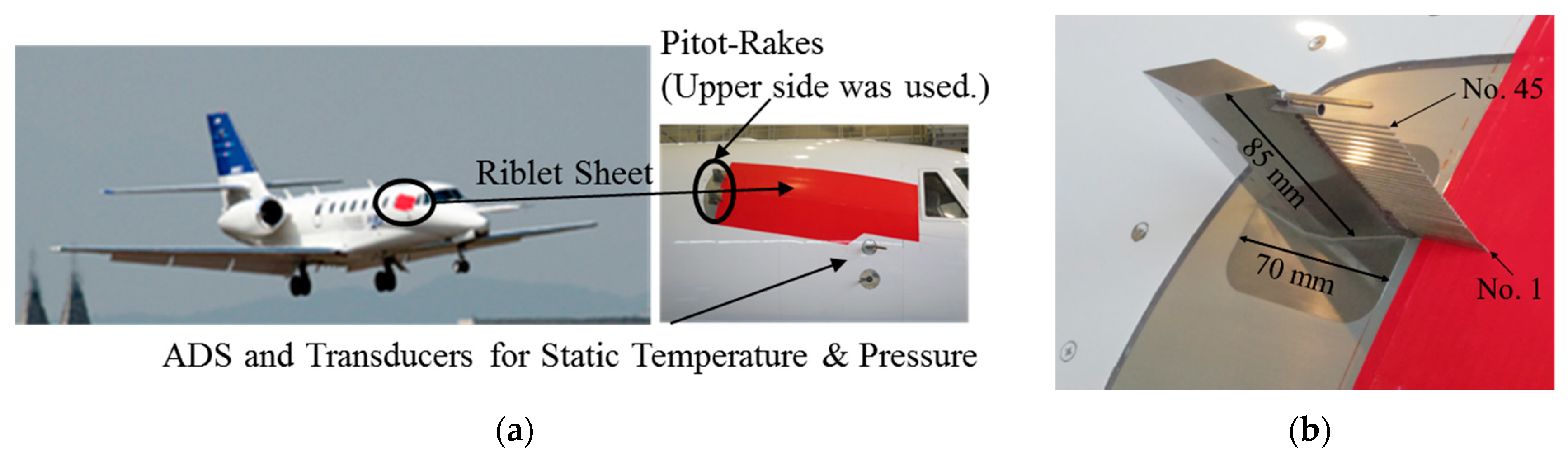
2.1. Flight Test Bed and Measurement System Onboard

Skin friction is one of the most difficult flow properties in aerodynamics to measure. Among various methodologies that can be applicable to measure the skin friction force, the pitot-rake measurement was employed in this study for the following reason. First, the direct estimation method from the change of the fuel consumption rate was not feasible as the riblet surface was only implemented on a very small part of the whole aircraft, and thus evaluating the fuel consumption rate with and without the riblet was extremely difficult over the measurement error caused by different flights [1]. A cantilever measurement system, which has been widely used to measure the skin friction force in wind tunnel experiments [30,31,32], is very sensitive to error caused by the configuration, such as a very small gap or misalignment. Optical measurement methods such as using oil flow measurement are also very difficult because the riblet width is very tiny [33,34,35]. Conversely, direct measurement of the velocity profile in the boundary layer by the pitot-rake measurement is reliable to measure the velocity profile with highly accurate pressure transducers [33,36]. The measured velocity profile is a time-averaged value as the pitot-rake measurement involves pneumatic probe systems.
Figure 1a shows the flight test bed and pitot-rakes with static pressure and temperature ports implemented on the airframe surface, and just in front of the pitot-rake. The pitot-rake was designed to have a rigid structure made of stainless steel and was constructed on the metal window surface, the original window of which was replaced with the metal surface so as to install the pitot-rake. The riblet portion is also shown in the figure. It should be noted that the riblet size is in the order of 100 μm; therefore, the measurable range would be from the log-law region to the outer region of the boundary layer. The details of the riblet will be described briefly in a later section. Two pitot-rakes were located behind the riblet sheet, which had a cord length of 1306 mm, an effective span length of 574 mm, and a thickness of approximately 100 μm.
Figure 1b shows a schematic of the pitot-rake, which consists of 45 single-hole probes for measuring pitot pressure to identify the boundary layer profile on the aircraft fuselage. The minimum probe diameter employed in the present study was 0.5 mm. The direction where the pitot-rakes were aligned was determined by assuming that the pitot-rakes were located on the streamline along the fuselage which was estimated by numerical simulation [17]. Note that an actual streamline can vary depending on flight conditions and, hence, the location of the pitot-rake may not be aligned with the flow. However, since the measurement in this study was conducted at steady cruise conditions where the angle of attack was near zero, the actual streamline was assumed to be close to that simulated by the computational analysis. Additionally, the pitot-rake was considered to measure the streamwise velocity of the flow accounting for past studies [37] that showed that the measurement accuracy was ensured up to the angle of attack of 20° at flight Mach number of 0.64 [37]. Furthermore, a calibration wind tunnel experiment, which was conducted prior to the flight experiment [23], showed that the uncertainty in measuring the pitot pressure for the designed pitot-rake can be negligible in the range of the angles of attack of less than ±5° [23]. Thus, the pitot-rake was considered to measure the streamwise velocity profile of the flow on the aircraft fuselage at targeted steady cruise flight conditions. The aft-part of the pitot-rake has a rhombus cross-section to avoid generating extra lift and to avoid vibration introduced by the unstable flow separation. The accuracy of the pitot-rake measurement was approximately 3.5% which was calculated as a maximum error level obtained as a ratio of 1σ over an average velocity value measured for 1-min duration for all probes.
The measurement system onboard the aircraft consisted of transducers for measuring pitot pressure, static pressure and static temperature, and the data recording system. Each measured signal was recorded by a commercially available laptop computer at a sampling frequency of 10 Hz.
The air-data system (ADS) was equipped in the vicinity of the aircraft forebody as shown in Figure 1a for sensing air-data such as Mach number, pressure, temperature, angle of attack, and angle of sideslip. The accuracy of sensing air-data was, for example, 0.4% for measuring Mach number.

2.2. Paint-Based Riblets

The paint-based riblet was attached on the surface of the fuselage as shown in Figure 1. The riblet was painted on aviation stickers. The riblet shape was a straight groove shape, the width of which is 170 μm. More details of the riblet used in the flight experiment can be found elsewhere [17,22,38] as this study emphasizes the interpolation of the boundary layer profiles measured under flight conditions.

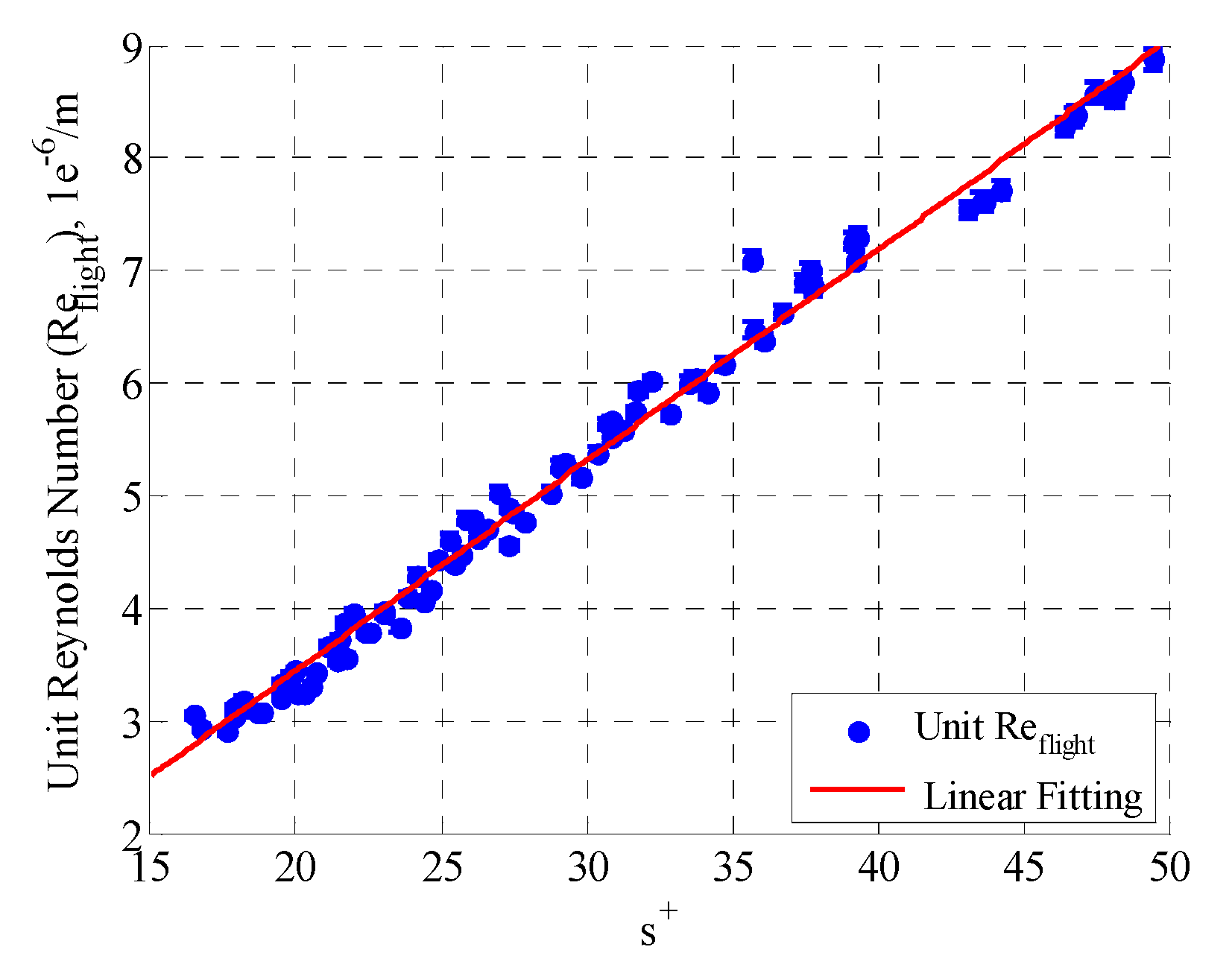
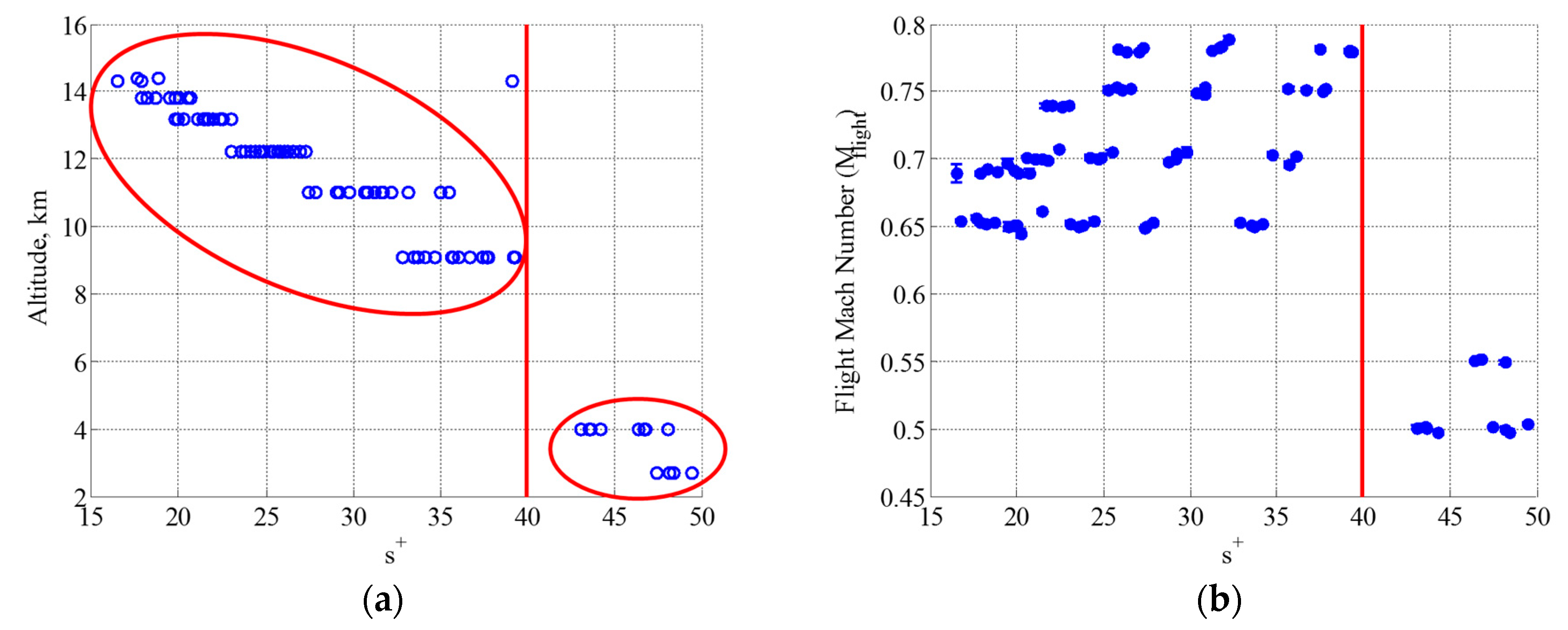
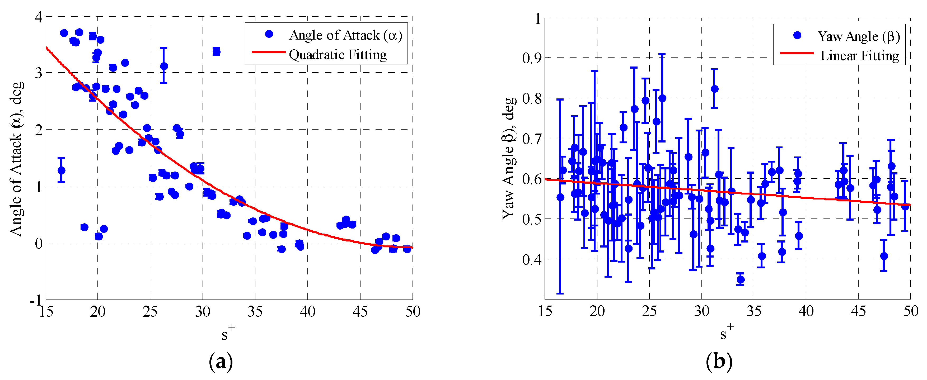
2.3. Test Conditions

Since the flight experiment was conducted as part of the FINE project’s study of the effectiveness of riblets in reducing skin friction drag, test conditions were determined based on certain physical parameters related to evaluating skin friction drag. The primary condition is expressed as Equation (1), which is a non-dimensional riblet width and essentially a Reynolds number based on the riblet width and friction velocity. This parameter was used to determine the flight Mach number, altitude, and other flight conditions.
s + = u τ · s ν = s ν 1 2 · c f · U 2 ¯
c f = 0.0592 · R e x 1 5
R e u = ρ · U μ = ρ μ · M · γ · R · T
The effectiveness of the riblet in reducing skin friction depends on the turbulent eddy size in the boundary layer and the riblet valley width; therefore, the effectiveness is strongly related to the Reynolds number. The Mach number dependence is generally small [39]. The unit Reynolds number based on the flight conditions is expressed as Equation (3) and the relationship between s+ and Reu (or Reflight) is presented in Figure 2. As seen in Figure 2, s+ has a linear relationship with Reu. The R2 value is 0.99 for those variables. In order to realize a wide range of flight conditions, the Reynolds number was varied by the variance of the flight Mach number and the flight altitude. The resultant flight altitude range was approximately 8900 ft. to 47,000 ft. with the unit Reynolds numbers of approximately 2.9–9.1 × 10⁶ (as presented in Figure 2) and the flight Mach numbers of 0.5–0.78. In total, six flights were performed during the flight test campaign.
Figure 3 shows the representative flight history conducted at a single flight in case of M = 0.65. Each flight involved several cruise conditions at a premised s+ condition for a duration of at least 60 s.
Figure 4 presents the relationships between certain variables and flight test conditions. Each data point is an averaged value made for a 60-s duration at each targeted cruise condition. The errorbar is the standard deviation (1σ) for the averaging duration. The Mach number and altitude ranges were mentioned before. Figure 4a shows the relationship between s+ and the flight altitude. As can be seen, the s+ value decreases nearly linearly with increasing flight altitude. Additionally, s+ distribution drastically changes across its value of 40 or the flight altitude range across approximately 4–8 km from sea level. Figure 4b shows the relationship between the flight Mach number and s+. While the flight Mach number is less sensitive to s+ as seen in Figure 4b, a low Mach number range (i.e., approximately M = 0.5) was implemented at low altitudes below approximately 8 km from sea level, and a high Mach number range was made at high altitudes in the altitude range of approximately 8 to 11 km from sea level.
Figure 5 plots the sensitivities of other variables (i.e., angle of attack, yaw angle, pressure, temperature) to s+. In each plot, a fitting curve is superimposed to identify the overall trend of the distribution. While the yaw angle has less sensitivity to s+, angles of attack, pressures, and temperatures clearly show a dependence on s+ to some extent. Among those property variables, the variables having an influence on interpolation postprocessing will be discussed in a later section, along with the response surface methodology.

3. Data Reduction Methodologies

This section presents an interpolation technique based on RSM to reconstruct the boundary layer profile, and the sensitivity of variables to the technique.

3.1. Application of Response Surface Methodology (RSM) to Flight Data

As mentioned above, such flow features as boundary layer profiles around the aircraft airframe cannot always be the same at a targeted flight condition due to the difference in remaining fuel, the resultant difference at the angle of attack, and atmospheric air conditions for each flight. This situation leads to difficulty in evaluating such testing devices as the riblets aimed at reducing skin friction drag. For example, in the case of evaluating the reduction of skin friction drag by using the riblets, a comparison can be made between a case not using riblets and a case using riblets. The datasets of both cases would be obtained at different flights. In order to properly compare a dataset (e.g., boundary layer profile) obtained at different flights by eliminating the influence of the flight conditional difference, an approach was taken to interpolate the data by using response surface methodology.
RSM consists of a group of mathematical and statistical techniques for empirical model building. The objective of RSM is to optimize a response or an output variable to some influential independent variables (input variables). RSM was originally developed to model experimental responses [40,41], but its application field was later expanded to the modelling of numerical experiments. An inaccuracy of RSM can be defined as measurement errors. The following describes the sequence of the interpolation approach conducted in this study based on RSM.
  • Reference Case
    (i)
    First, flight experimental data obtained with a smooth wall surface on the aircraft airframe without involving any flow control device such as riblets were considered as reference data to be compared. The dataset for the reference case (as well as other flight cases) contains pitot pressure data and flight condition data such as Mach number, Reynolds number, etc. (hereinafter, flight data) measured by ADS onboard. The pressure coefficient based on pitot pressure divided by flight dynamic pressure was considered the primary parameter of interest and is expressed as follows:
    C p = P p i t o t r e f P r e f 1 2 · γ P r e f · M r e f 2
    From Equation (4), the pitot pressure at each pitot-probe is obtained as follows:
    p p i t o t r e f = C p r e f · ( 1 2 γ p r e f M r e f 2 ) + p r e f
    Based on Equation (5) and assuming the isentropic flow process, the Mach number at each pitot-probe is obtained by Equation (6) by further assuming that the pitot pressure at each pitot-probe is considered to be the local total pressure at each probe tip. Here, an assumption was made that no total pressure loss was involved in the shock wave formation in front of each pitot-probe, since the entire flowfield is considered to be subsonic in accounting for flight speed conditions.
    M p i t o t r e f = ( 2 γ 1 ) { ( p p i t o t r e f p r e f ) γ 1 γ 1 }
    Rewriting Equation (6) in terms of U-velocity yields the U-velocity (Upitot) at each pitot-probe as Equation (7).
    U p i t o t r e f = M p i t o t r e f · γ · R · T 0 · ( 1 + γ 1 2 M p i t o t r e f 2 ) 1
  • Compared case
    (ii)
    Similar to the reference case, the pressure coefficient for the compared case, C p c o m , is created by pitot pressures and flight data for the compared case (Equation (8)).
    C p c o m = p p i t o t c o m p c o m 1 2 γ p c o m M c o m 2
    (iii)
    Assuming that the pressure coefficient at each pitot-probe can be expressed by using some measured variables yields an expression of C p c o m shown as Equation (9).
    C p c o m = f ( x 1 ,   x 2 ,   ,   x n ) + ε
    Here, x1, x2, … are variables obtained by flight experiments such as α, Reu, β, U, T0∞, and P0∞. Each variable is independent of each other. ε is the uncertainty arising from reconstructing Cp with the interpolation technique.
    (iv)
    Equation (9) is then expressed by applying response surface methodology as follows. Since the fitting curve being used for interpolation would be a curvature response, the 3rd-degree response surface model was employed. Detailed reason behind the usage of the 3rd-degree response surface model will be presented in a later section along with a comparison of interpolated boundary layer profile using the 2nd-degree response surface model. Note that this process is only meaningful for the compared case; the interpolated reference data are identical to the original reference data.
    C p c o m = C p f i t = a 0 + i = 1 N a i x i + i = 1 N i j N b i , j x i x j + ε
    Here, N is the total number of variables and each variable is chosen as, for instance, N = 4, x1 = M, x2 = Re, x3 = P, and x4 = α. a and b are coefficients for calculating the response surface. It should be noted that each variable would be non-dimensionalized prior to making a fitting curve using Equation (10). The cross terms in Equation (10) appear to introduce the curvature of the response surface since the fitting curve for this case would not be linear.
    (v)
    Coefficients appearing in Equation (10) can be obtained by expressing Equation (10) in matrix notation as follows:
    C p f i t = X * A + ε = ( 1 x 1 , k 1 x n , k ) ( a 1 a n ) + ( ε 1 ε n ) .
    where C p f i t is a vector of the parameter being reconstructed by the fitting dataset for interpolation, X is the matrix of values of the design variables at each flight condition, A is the vector of tuning parameters, and ε is a vector of errors inherent in the curve fitting using the response surface model (equivalent to the one expressed in Equation (10)). n is the total number of experimental cases and k is the total number of variables. A can be estimated using the least-square error method as:
    A = ( X T * X ) 1 X T
    (vi)
    The interpolated pressure coefficient for compared case C p f i t c o m ( x 1 ,   x 2 ,   ,   x N ) , which is interpolated for equivalent flight conditions of the reference case (x1~xN)|ref, is now obtained.
    (vii)
    Then the interpolated pitot pressure is expressed as:
    p p i t o t c o m i n t e r p o l a t e d = C p f i t c o m · ( 1 2 γ p r e f M r e f 2 ) + p r e f
    The interpolated pitot pressure and Mach number at each pitot-probe are expressed using the above relationships and isentropic relationships as follows:
    M p i t o t c o m _ i n t e r p o l a t e d = ( 2 γ 1 ) { ( p p i t o t c o m i n t e r p o l a t e d p _ r e f ) γ 1 γ 1 }
    U p i t o t c o m i n t e r p o l a t e d = M p i t o t c o m i n t e r p o l a t e d · γ · R · T 0 · ( 1 + γ 1 2 M p i t o t c o m i n t e r p o l a t e d 2 ) 1
Thus, the interpolated distributions of pitot pressure and Mach number at each pitot-probe are obtained.

3.2. Governing Parameters and Data Screening

In applying RSM for the interpolation of the boundary layer profile, many combinations between the fitting degree of the response surface model (N = 2, 3, 4, …) and the flight data (M, Re, …) may be possible. For instance, a sufficiently large number of datasets would increase the accuracy of the fitting curve in response surface model by using as many variables as possible. However, available data points would generally be limited, such as the five points available for the reference wall case at the premised Mach number of 0.70 in this study. Therefore, some additional consideration was given on selecting the governing parameters. The order of the response surface curve was chosen as 3 to improve the fitting accuracy as compared to the 2nd-degree fitting that is generally used [41]. A comparison of interpolated boundary layer profiles obtained by the 2nd-degree response surface model and that by the 3rd-degree response surface model will be presented in a later section.
Figure 6 presents the relationship between each variable and Cp at the outmost probe height (probe number 45). Cp was created using Equation (4). A representative curve fit is also superimposed in each figure. The measured value at the outmost probe height was considered to represent the freestream value. As seen in Figure 6, each variable has a certain sensitivity on Cp. Here, flight data obtained at the premised fight Mach number of 0.70 are plotted as an example. Note that the aforementioned RSM will be applied to flight test conditions at a single premised flight for the Mach number cases. Note that other probe height data showed a similar trend to that at probe number 45. A weak correlation is shown against Cp for the angle of attack, yaw angle, and temperatures. In contrast, the flight Mach number, pressures, and unit Reynolds number have a certain linear sensitivity.
In order to further investigate the reasons behind those observed behaviors of variables, some governing parameters responsible for reconstructing the pressure coefficient are explored. The primary parameter of the pressure coefficient is again shown below.
C p ,   a t   e a c h   h e i g h t = P p i t o t ,   a t   e a c h   h e i g h t P 1 2 · γ P 0 · M 2 · ( 1 + γ 1 2 M 2 ) γ γ 1 = M e a s u r e d   V a l u e F l i g h t   D a t a
Here, the numerator is the measured data and the denominator is the flight data obtained by the ADS. Since the pitot pressure is normalized by the flight data, the flight Mach number and total atmospheric pressure that appear in the denominator would have an influential impact on the scaling of Cp. Based on the linear relationships for the Mach number, unit Reynolds number, and the pressures shown in Figure 6, and on the definition of Cp described above, and by considering that the unit Reynolds number is a combination of other parameters, the influential parameters are evidently the flight Mach number and the pressures. Therefore, these two parameters were considered as governing parameters and the other parameters were screened out.

3.3. Response Surface Model (Interpolation of Boundary Layer Profile)

Figure 7 shows the response surface model being used to interpolate the dataset. The model was reconstructed based on the flight Mach number and total pressure. The original flight experimental data are superimposed as black-colored dots for a comparison. The experimental data indicate the case for targeted flight Mach number of 0.65 and measured at the probe numbers 5 (: near the wall surface) and 45 (: near the outer edge of the boundary layer). The corresponding response surface models for probe numbers 5 and 45 are presented. The response surface model reconstructs the Cp distribution through the interpolation technique using RSM as a function of the flight Mach number and total pressure with fine accuracy, the details of the uncertainty in reconstructing the boundary layer profile by using the response surface model will be presented in a later section. It should be noted that the response surface model must not involve any extrapolations as the extrapolated data point could cause a massive error. In order to ensure that the generated response surface does not involve any extrapolations, constraints were added. The constrains were defined based on the minimum and maximum values of primary variable Cp obtained in the actual flight data at targeted steady cruise flight conditions. If the reconstructed dataset in the response surface curve, which is shown in Figure 7, exceeded the constrained area, the exceeded data points were constrained to be a boundary value of the constrained area. Thus, the reconstruction of the profile ensured the use only of the interpolation and did not involve any extrapolation. This process strengthens the robustness of the interpolation as it ensures using only interpolation and avoid potential errors by using the extrapolation.

4. Results and Discussion

This section discusses the insights gained from the interpolation technique using response surface methodology, which cover the following topics of interest: uncertainty and accuracy of interpolation for flight experimental data measured at different flights.

4.1. Accuracy of Interpolation

Figure 8a compares a representative Cp profile of original smooth wall data with that of the interpolated profile. The flight experimental conditions for the presented case were a flight Mach number (M) of 0.65, a 2° angle of attack (α), total ambient pressure (P) of 22.4 kPa, and total ambient temperature (T) of 235.0 K. Note that the reconstructed interpolated curve for this reference case should be identical to the original distribution since the same dataset was used for the interpolation. Therefore, the difference (i.e., maximum difference) between the original and interpolated curves is an uncertainty (ε) arising from the interpolation. This maximum uncertainty caused by interpolation using the response surface model for reconstructing the profile will be described in detail later in this section.
Figure 8b plots the maximum uncertainty expressed by the maximum difference between the original and interpolated profiles for all measured points in percentage for all test cases. The maximum uncertainty by the reconstruction using the response surface model stays within approximately 4.43 × 10⁻⁹%. Therefore, ε ≤ 4.43 × 10⁻⁹%. The maximum uncertainty by using the 2nd-degree response surface model was approximately 0.23% for the same calculation condition used for the 3rd-degree response surface model. Thus, with this level of uncertainty, the interpolation method using the 3rd-degree response surface model reconstructs the boundary layer profile on the aircraft fuselage well.
Figure 9 compares the profiles of Cp (Figure 9a) and U-velocity (Figure 9b) between two smooth wall cases obtained at different flights under the same premised s+ condition (where ‘Ref’ denotes a flight condition with M = 0.65, α = 2.68°, s+ = 23.8, and ‘Com’ denotes a flight condition with M = 0.65, α = 2.59°, s+ = 23.0). ‘Original’ and ‘interpolated’ profiles denote the raw profile and interpolated profile, respectively. For example, in Figure 9a, Ref (Original) represents the original boundary layer profile data for the reference case; and Ref (Interpolated) represents the interpolated data for the reference case. The same rule is applied to the other dataset. The 2nd-degree response surface model with two variables: x1 = P0∞ and x2 = M was employed here. As seen in Figure 9a, discrepancy between the original and interpolated profiles is evident around the probe height in the region of 20–30 mm. This region approximately corresponds to an inflection point of the boundary layer profile exists. Therefore, qualitatively, the 2nd-degree response surface model can roughly interpolate the profile though it involves some error as seen in Figure 9. The maximum discrepancy between the reference and compared cases in their interpolated profiles was found to be approximately 0.1% for Cp and approximately 2.6% for U-velocity.
Figure 10 compares the profiles of Cp (Figure 10a) and U-velocity (Figure 10b) between two smooth wall cases as presented in Figure 9. The 3rd-degree response surface model with two variables: x1 = P0∞ and x2 = M was employed here. As in the interpolation with the 2nd-degree response surface model, the interpolation with the 3rd-degree response surface model can interpolate the profile well. Obviously, the 3rd-degree response surface model reconstructs the boundary layer profile better than that with the 2nd-degree response surface model as the error appeared in the region around the probe height of 20 mm–30 mm in Figure 9 is not seen here. The maximum discrepancy between the reference and compared cases in their interpolated profiles was found to be in the order of 10−7% for Cp and less than 2.6% for U-velocity. Accounting for the results shown in Figure 9 and Figure 10, the 3rd-degree response surface model can interpolate the entire boundary layer profile better than the 2nd-degree response surface model.
Figure 11a presents the uncertainty in the interpolation with the 3rd-degree response surface model for all other flight conditions. Each data point expressing an average difference between the profiles obtained at two flights was derived as shown in Figure 9. Average differences with regard to U-velocity not using the interpolation and using the interpolation for all pitot-probes between the reference case and compared case are presented. As seen from average differences for data not using the interpolation and using the interpolation in Figure 11, error level is reduced from 0.84% to 0.39% by implementing the interpolation. The maximum error after interpolation is 1.8% and the average error level is approximately 0.39%. The maximum error level is then considered to be cumulative error by implementing the interpolation. Note that the total uncertainty could contain uncertainty in the freestream condition, and will be discussed in the next section. As a comparison, the 2nd-degree response surface model yielded the maximum error level of approximately 1.8% and the average error level of approximately 0.54%, as shown in Figure 11a. The 3rd-degree response surface model was, therefore, employed in this study due to a reduced error level compared to the 2nd-degree response surface model.
As the average error value appeared to scatter to some extent against s+ value since the available dataset was limited, Figure 11b presents a histogram of the average error in U-velocity. A normal distribution is superimposed with the mean and standard deviation values obtained from the error values plotted in Figure 11a for U-velocity. The distribution is normalized by its maximum value so that the peak value shows unity. Approximately 68.3% of the error population appears within an error value of 0.39%, indicating that only a small population could have a large error.

4.2. Uncertainty Analysis

As mentioned in the Introduction section, the reduction of skin friction drag appears to be in the order of several percent (e.g., using a riblet surface). Therefore, it is vital to quantify the uncertainty inherent in the measurement of physical properties of interest, such as U-velocity distribution and in the postprocessing of the measured raw datasets. Table 1 summarizes the possible uncertainty sources inherent in both measurement and postprocessing. Each measured value of flight data including atmospheric air data and pitot pressure data was averaged for a duration of 1 min, and those associated errors were considered to be 1σ for the averaging duration as mentioned in the previous section. The RSM error obtained from the interpolation described in the previous section was the governing error source. The cumulative error was approximately 4.1%, which corresponds to ε in Equation (9). Thus, the boundary layer profile based on U-velocity obtained from pitot-rake measurement under flight conditions was interpolated by applying response surface methodology within an uncertainty of 4.1%.

5. Conclusions

RSM was applied to interpolate the boundary layer’s U-velocity profile on the aircraft fuselage measured in flight using pitot-pressure measurement. The flight testing was conducted as part of the FINE project aimed at demonstrating the reduction of skin friction drag by using a paint-based riblet. Despite the same premised flight test conditions with regard to the Reynolds number based on aircraft flight speed and ambient conditions in flight, slight variations in flight attitude or atmospheric air conditions measured by the air-data sensing system onboard would cause a difference in features of the boundary layer profile, since the local freestream velocity in the vicinity of the measurement station of the pitot-rakes would be different due to the difference in atmospheric air conditions. This concern makes it difficult for an accurate comparison in the boundary layer profiles measured at different flights; and thus some kind of skin friction drag reduction technique such as one using riblets is needed for an accurate and careful evaluation. In other words, it makes it difficult to distinguish whether the difference in the boundary layer profile appeared due to a slight difference in different flight conditions or by using the riblets. To ensure an accurate evaluation of the reduction of skin friction drag or the change of the boundary layer profile by using the riblets, an interpolation approach was applied to eliminate the uncertainty caused by the flight conditional difference.
The interpolation technique based on response surface methodology used a pitot-pressure coefficient as a primary parameter. The reference smooth wall surface and the riblet wall surface were compared with regard to the boundary layer’s U-velocity profile. By using response surface methodology applied to the reference smooth wall case, the boundary layer’s U-Velocity profile was reconstructed within an uncertainty of 4.1% for a flight Mach number range of 0.5 to 0.78. As the reduction of skin friction drag by using the riblets would be in the order of several percent up to approximately 10%, this accuracy facilitates an accurate evaluation of the reduction of skin friction by using riblets. Thus, the proposed interpolation method facilitated a successful interpolation of the flight experimental data.
In future work, a more systematic study to screen the variables will be undertaken to make the proposed method more robust. Additionally, the quantitative translation from Δu+, which will be gained by comparing the boundary layer profiles between cases of with and without using riblets, to the actual amount of reduction of skin friction drag, will be obtained.

Author Contributions

Conceptualization, H.T. is responsible for the entire work from conceptualization, establishing methodology, data analysis, and writing the original manuscript entirely; M.K. managed the overall project and reviewed; H.I. and M.S. worked on raw data processing obtained from the flight experiment.

Funding

This research received no external funding.

Acknowledgments

This study was conducted as part of the Flight Investigation of Skin-Friction Reduction Eco-Coating (FINE) project by JAXA’s Aeronautical Technology Directorate. The authors wish to thank Masato Asai and Ayumi Inazawa at Tokyo Metropolitan University, Shihoko Endo and Kaoru Iwamoto at the Tokyo University of Agriculture and Technology, and Ryoko Shinohara at O-WELL corporation for the riblet design. The authors would also like to acknowledge Atsushi Yasuda and Yukio Oizumi at Diamond Air Service, Inc., and Hiroshi Tomita, Ikuya Shirota, Hideki Sato, Ryoji Hirai, Masayuki Nagae, Takehiro Kumagai, Wataru Mukaidani, and Masayoshi Noguchi at JAXA for conducting the flight testing. Finally, the authors would like to thank Yoshikazu Makino and Kouichiro Tani for their insightful help in research collaboration across directorates.

Conflicts of Interest

The authors declare no conflict of interest.

Nomenclature

cflocal skin friction coefficient
Cppressure coefficient
MMach number
quncertainty
Rgas constant
ReReynolds number
swidth of riblet, μm
s+non-dimensional width of riblet
Ttemperature, K or °C
Ustreamwise velocity component (U-velocity), m/s
Uτfriction velocity
xcoordinate in streamwise direction
ycoordinate in spanwise direction
zcoordinate in vertical direction
αangle of attack, deg
βyaw angle or angle of sideslip, deg
δboundary layer thickness, mm
εtiny amount or uncertainty
γspecific heat ratio
μdynamic viscosity
νkinematic viscosity, m2/s
ρdensity, kg/m3
σstandard deviation
Subscripts
0stagnation condition
comcompared case
fitfitted data
flightflight condition
i, jindex number
interpolatedinterpolated data
pitotpitot-rake data
refreference case
sstatic condition
totaltotal value
uunit value
freestream condition

References

  1. Szodruch, J. Viscous Drag Reduction on Transport Aircraft Reno. In Proceedings of the AIAA 29th Aerospace Sciences Meeting, Reno, NV, USA, 7–10 January 1991. AIAA Paper 91-0685. [Google Scholar]
  2. Yousefi, K.; Saleh, R. Three-dimensional suction flow control and suction jet length optimization of NACA 0012 wing. Meccanica 2015, 50, 1481–1494. [Google Scholar] [CrossRef] [Green Version]
  3. Zhang, Z.Y.; Zhang, W.L.; Chen, Z.; Sun, X.H.; Xia, C.C. Suction control of flow separation of a low-aspect-ratio wing at low Reynolds-number. Fluid Dyn. Res. 2018, 50, 065504. [Google Scholar]
  4. Yousefi, K.; Saleh, R.; Zahedi, P. Numerical study of blowing and suction slot geometry optimization on NACA 0012 airfoil. J. Mech. Sci. Technol. 2014, 28, 1297–1310. [Google Scholar] [CrossRef] [Green Version]
  5. You, D.; Moin, P. Active control of flow separation over an airfoil using synthetic jets. J. Fluids Struct. 2008, 24, 1349–1357. [Google Scholar] [CrossRef]
  6. Wang, H.; Zhang, B.; Qiu, Q.; Xu, X. Flow control on the NREL S809 wind turbine airfoil using vortex generators. Energy 2017, 118, 1210–1221. [Google Scholar] [CrossRef]
  7. Saravi, S.S.; Cheng, K. A Review of Drag Reduction by Riblets and Micro-Textures in the Turbulent Boundary Layers. Eur. Sci. J. 2013, 9, 62–81. [Google Scholar]
  8. Walsh, M.J. Riblets, Viscous Drag Reduction in Boundary Layers; Bushness, H., Ed.; Progress in Astronautics and Aeronautics; American Institute of Aeronautics and Astronautics: Washington, DC, USA, 1989; Volume 123, pp. 203–261. [Google Scholar]
  9. Walsh, M.J. Riblets as a Viscous Drag Reduction Technique. AIAA J. 1983, 21, 485–486. [Google Scholar] [CrossRef]
  10. Sareen, A.; Deters, R.W.; Henry, S.P.; Selig, M.S. Drag reduction using riblet film applied to airfoils for wind turbines. J. Sol. Energy Eng. 2014, 136, 021007. [Google Scholar] [CrossRef]
  11. Raayai-Ardakani, S.; McKinley, G.H. Drag reduction using wrinkled surfaces in high Reynolds number laminar boundary layer flows. Phys. Fluids 2017, 29, 093605. [Google Scholar] [CrossRef]
  12. Sasamori, M.; Iihama, O.; Mamori, H.; Iwamoto, K.; Murata, A. Parametric Study on a Sinusoidal Riblet for Drag Reduction by Direct Numerical Simulation. Flow Turbul. Combust. 2017, 99, 47–69. [Google Scholar] [CrossRef]
  13. Bushnell, D.M.; Hefner, J.N.; Ash, R.L. Effect of Compliant Wall Motion on Turbulent Boundary Layers. Phys. Fluids 1977, 20, S31–S48. [Google Scholar] [CrossRef]
  14. Suzuki, Y.; Kasagi, N. Turbulent Drag Reduction Mechanism Above a Riblet Surface. AIAA J. 1994, 32, 1781–1790. [Google Scholar] [CrossRef]
  15. Dean, B.; Bhushan, B. Shark-Skin Surfaces for Fluid-Drag Reduction in Turbulent Flow: A Review. Philos. Trans. R. Soc. A 2010, 368, 4775–4806. [Google Scholar] [CrossRef] [PubMed]
  16. Viswanath, P.R. Aircraft Viscous Drag Reduction Using Riblets. Prog. Aerosp. Sci. 2002, 38, 571–600. [Google Scholar] [CrossRef]
  17. Okabayashi, K.; Matsue, T.; Asai, M. Development of Turbulence Model to Simulate Drag Reducing Effects of Riblets. J. Jpn. Soc. Aeronaut. Space Sci. 2016, 64, 41–49. (In Japanese) [Google Scholar]
  18. Sawyer, W.; Winter, K. An Investigation of the Effect on Turbulent Skin Friction of Surface with Streamwise Grooves. In Turbulent Drag Reduction by Passive Means; The Royal Aeronautical Society: London, UK, 1987; pp. 330–362. [Google Scholar]
  19. Walsh, M.J. Turbulent Boundary Layer Drag Reduction Using Riblets. In Proceedings of the AIAA 20th Aerospace Sciences Meeting, Orlando, FL, USA, 11–14 January 1982. AIAA Paper 82-0169. [Google Scholar]
  20. Bechert, D.W.; Bruse, M.; Hage, W.; Van Der Hoeven, J.G.T.; Hoppe, G. Experiments on Drag-Reducing Surfaces and their Optimization with an Adjustable Geometry. J. Fluid Mech. 1997, 338, 59–87. [Google Scholar] [CrossRef]
  21. MBB Transport Aircraft Group. Microscopic Rib Profiles Will Increase Aircraft Economy in Flight. Aircr. Eng. 1988, 60, 11. [Google Scholar] [CrossRef]
  22. Kurita, M.; Nishizawa, A.; Okabayashi, K.; Koga, S.; Kwak, T.; Nakakita, K.; Naka, Y. FINE: Flight Investigation of Skin-Friction Reducing Eco-Coating. In Proceedings of the 54th Aircraft Symposium, Toyama, Japan, 31 October–2 November 2016. JSASS-2016-5180 (In Japanese). [Google Scholar]
  23. Koga, S.; Kurita, M.; Iijima, H.; Okabayashi, K.; Nishizawa, A.; Takahashi, H.; Endo, S. Wind Tunnel Tests for Measurement System Design of Flight Investigation of Skin-Friction Reducing Eco-Coating (FINE). In Proceedings of the 54th Aircraft Symposium, Toyama, Japan, 31 October–2 November 2016. JSASS-2016-5105 (In Japanese). [Google Scholar]
  24. Rosenbaum, B.; Schulz, V. Response Surface Methods for Efficient Aerodynamic Surrogate Models. Comput. Flight Test. 2013, 123, 113–129. [Google Scholar]
  25. Sevant, N.E.; Bloor, M.I.G.; Wilson, M.J. Aerodynamic Design of a Flying Wing Using Response Surface Methodology. J. Aircr. 2000, 37, 562–569. [Google Scholar] [CrossRef]
  26. Zhang, M.; He, L. Combining Shaping and Flow Control for Aerodynamic Optimization. AIAA J. 2015, 53, 888–901. [Google Scholar] [CrossRef]
  27. Papila, M.; Haftka, R.T. Response Surface Approximations: Noise, Error Repair, and Modeling Errors. AIAA J. 2000, 38, 2336–2343. [Google Scholar] [CrossRef]
  28. Madsen, J.; Shyy, W.; Haftka, R.T. Response Surface Techniques for Diffuser Shape Optimization. AIAA J. 2000, 38, 1512–1518. [Google Scholar] [CrossRef]
  29. Walsh, M.J.; Sellers, W.L., III; McGinley, C.B. Riblet Drag at Flight Conditions. J. Aircr. 1989, 26, 570–575. [Google Scholar] [CrossRef]
  30. Takahashi, H.; Tomioka, S.; Sakuranaka, N.; Tomita, T.; Kuwamori, K.; Masuya, G. Effects of Plume Impingements of Clustered Nozzles on the Surface Skin Friction. J. Propuls. Power 2015, 31, 485–495. [Google Scholar] [CrossRef]
  31. Marshakov, A.V.; Scheta, J.A.; Kiss, T. Direct Measurement of Skin Friction in a Turbine Cascade. J. Propuls. Power 1996, 12, 245–249. [Google Scholar] [CrossRef]
  32. Allen, J.M. An Improved Sensing Element for Skin-Friction Balance Measurements. In Proceedings of the AIAA 18th Aerospace Sciences Meeting, Pasadena, CA, USA, 14–16 January 1980. AIAA Paper 1980-0049. [Google Scholar]
  33. Walsh, M.J.; Sellers, W.L.; McGinley, C.B. Riblet Drag Reduction at Flight Conditions. In Proceedings of the AIAA 6th Applied Aerodynamics Conference, Williamsburg, VA, USA, 6–8 Junuary1988. AIAA Paper 88-2554. [Google Scholar]
  34. Liu, T. Extraction of Skin-Friction Fields from Surface Flow Visualizations as an Inverse Problem. Meas. Sci. Technol. 2013, 24, 124004. [Google Scholar] [CrossRef]
  35. Bottini, H.; Kurita, M.; Iijima, H.; Fukagata, K. Effects of Wall Temperature on Skin-Friction Measurements by Oil-Film Interferometry. Meas. Sci. Technol. 2015, 26, 105301. [Google Scholar] [CrossRef]
  36. Mclean, J.D.; George-Falvy, D.N.; Sullivan, P.P. Flight-Test of Turbulent Skin-Friction Reduction by Riblets. In Turbulent Drag Reduction by Passive Means; The Royal Aeronautical Society: London, UK, 1987; pp. 408–424. [Google Scholar]
  37. Larson, T.J. Evaluation of a Flow Direction Probe and a Pitot-Static Probe on the F-14 Airplane at High Angles of Attack and Sideslip; NASA Technical Memorandum 84911; National Aeronautics and Space Administration: Washington, DC, USA, 1984.
  38. Kurita, M.; Nishizawa, A.; Kwak, D.; Iijima, H.; Iijima, Y.; Takahashi, H.; Sasamori, M.; Abe, H.; Koga, S.; Nakakita, K. Flight Test of a Paint-Riblet for Reducing Skin-Friction. In Proceedings of the AIAA 2018 Applied Aerodynamics Conference, Atlanta, GA, USA, 25–29 Junuary 2018. AIAA paper 2018-3005. [Google Scholar]
  39. Bushnell, D.M.; Hefner, J.; Walsh, M.J. Viscous Drag Reduction in Boundary Layers; American Institute of Aeronautics and Astronautics, Inc.: Reston, VA, USA, 1990. [Google Scholar]
  40. Box, G.E.P.; Draper, N.R. Empirical Model-Building and Response Surfaces; Wiley: New York, NY, USA, 1987. [Google Scholar]
  41. Khuri, A.I.; Mukhopadhyay, S. Response Surface Methodology. Wires Comput. Stat. 2010, 2, 128–149. [Google Scholar] [CrossRef]
Figure 1. (a) Japan Aerospace Exploration Agency (JAXA) flight test bed and riblet surface attached on the aircraft surface; and (b) schematic of pitot-rake attached on outer surface of an aircraft.
Applsci 08 02320 g001
Figure 2. Relationship between s+ and unit Reynolds number.
Applsci 08 02320 g002
Figure 3. Representative flight history showing flight Mach numbers and altitudes.
Applsci 08 02320 g003
Figure 4. Relationship between each variable and test conditions: (a) flight altitude and s+; (b) Mach number and s+.
Applsci 08 02320 g004
Figure 5. Sensitivities of flight conditions on s+: (a) angle of attack; (b) yaw angle, (c) pressure; (d) temperature.
Applsci 08 02320 g005aApplsci 08 02320 g005b
Figure 6. Sensitivities of each variable on Cp (at outmost probe height): (a) angle of attack; (b) yaw angle; (c) flight Mach number; (d) unit Reynolds number; (e) total and static pressures; (f) total and static temperatures.
Applsci 08 02320 g006
Figure 7. Data interpolation using the response surface model reconstructed based on flight Mach number and total pressure (original experimental data are superimposed for comparison): (a) probe No. = 5; (b) probe No. = 45.
Applsci 08 02320 g007
Figure 8. (a) Example case (M = 0.65, α = 2°, P = 22.4 kPa, T = 235.0 K) of the original Cp profile superimposed with the interpolated profile; and (b) maximum uncertainty presented in percentage among all pitot-probes for all measured flight cases caused by interpolation, along with flight experimental data for smooth wall cases.
Applsci 08 02320 g008
Figure 9. Comparison of profiles for smooth wall cases at two different flights (where ‘Ref’ denotes a condition with M = 0.65, α = 2.68°, s+ = 23.8, and ‘Com’ denotes a condition with M = 0.65, α = 2.59°, s+ = 23.0): (a) Cp; (b) U-velocity. Second-egree response surface model with two variables: x1 = P0∞ and x2 = M was employed.
Applsci 08 02320 g009
Figure 10. Comparison of profiles for smooth wall cases at two different flights (where ‘Ref’ denotes a condition with M = 0.65, α = 2.68°, s+ = 23.8, and ‘Com’ denotes a condition with M = 0.65, α = 2.59°, s+ = 23.0): (a) Cp; (b) U-velocity. Third-degree response surface model with two variables: x1 = P0∞ and x2 = M was employed.
Applsci 08 02320 g010
Figure 11. (a) Average difference for U-velocity compared between reference case and compared case plotted against s+; and (b) histogram of average error in U-velocity.
Applsci 08 02320 g011
Table 1. Summary of possible uncertainty sources.
Uncertainty SourceSymbolValue, %Note
Total pressureq10.025Atmospheric air pressure measured by the air-data sensing system onboard
Mach numberq21.01Obtained by the air-data sensing system onboard
Pitot measurementq33.5Max. percent uncertainty obtained as 1σ over an averaged value for 1-min duration for all probes
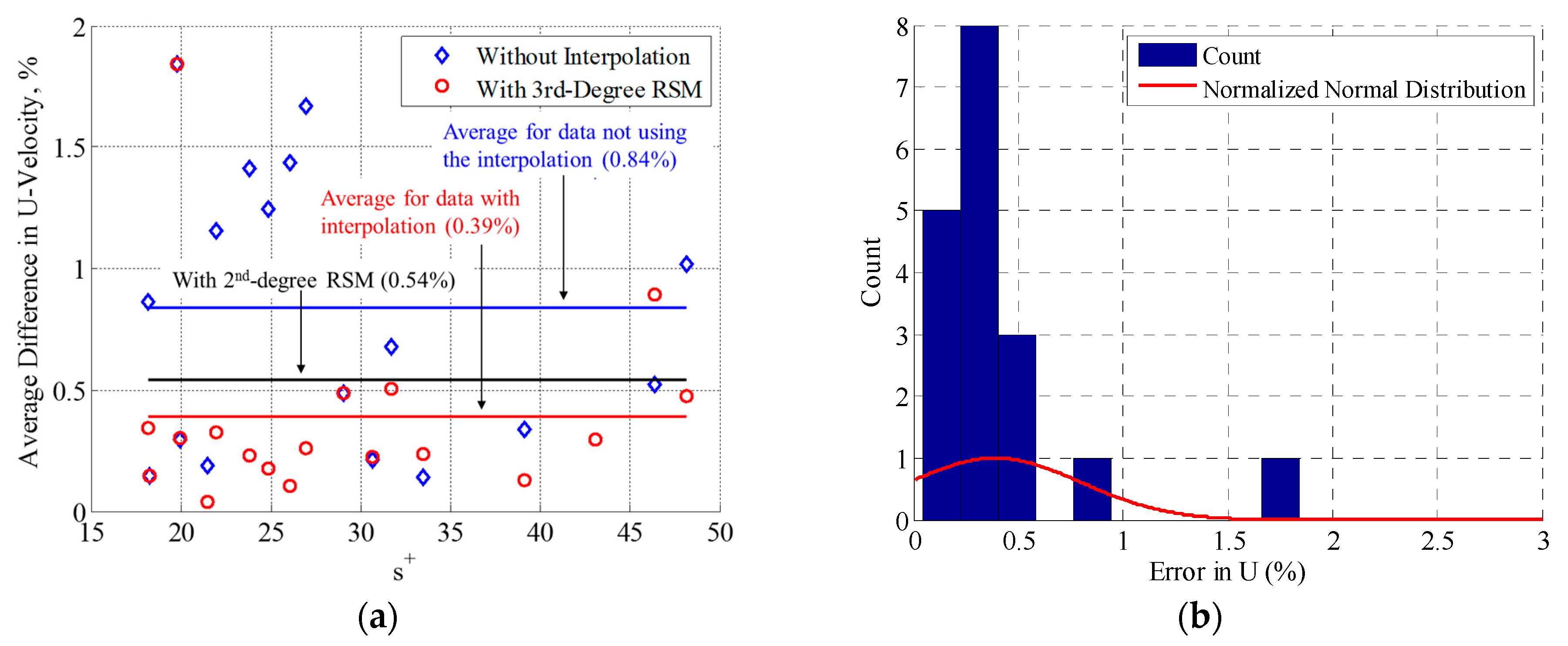
Response surface methodology (RSM) (Interpolation)q41.8Uncertainty obtained from Figure 10, including pitot pressure measurement error
Cumulative error (Total uncertainty)qtotal4.1 (4.06)Total uncertainty and corresponding to ε in Equation (9)

