Personalized HRTF Modeling Based on Deep Neural Network Using Anthropometric Measurements and Images of the Ear

Abstract

This paper proposes a personalized head-related transfer function (HRTF) estimation method based on deep neural networks by using anthropometric measurements and ear images. The proposed method consists of three sub-networks for representing personalized features and estimating the HRTF. As input features for neural networks, the anthropometric measurements regarding the head and torso are used for a feedforward deep neural network (DNN), and the ear images are used for a convolutional neural network (CNN). After that, the outputs of these two sub-networks are merged into another DNN for estimation of the personalized HRTF. To evaluate the performance of the proposed method, objective and subjective evaluations are conducted. For the objective evaluation, the root mean square error (RMSE) and the log spectral distance (LSD) between the reference HRTF and the estimated one are measured. Consequently, the proposed method provides the RMSE of −18.40 dB and LSD of 4.47 dB, which are lower by 0.02 dB and higher by 0.85 dB than the DNN-based method using anthropometric data without pinna measurements, respectively. Next, a sound localization test is performed for the subjective evaluation. As a result, it is shown that the proposed method can localize sound sources with higher accuracy of around 11% and 6% than the average HRTF method and DNN-based method, respectively. In addition, the reductions of the front/back confusion rate by 12.5% and 2.5% are achieved by the proposed method, compared to the average HRTF method and DNN-based method, respectively.

1. Introduction

The research and development of virtual reality (VR) and augmented reality (AR) have made significant progress over the last several decades. For the successful realization of VR/AR systems, it has been known that spatial sound or three-dimensional (3D) sound is an important component for enhancing the immersive quality of the systems when combined with video [1].

To generate such spatial sound, spatial cues from the human auditory system have been studied. The principle of spatial hearing is based on binaural and monaural cues [2]. Binaural cues imply the differences between two ears, including the time difference of arrival and the intensity difference between two ears, which are respectively referred to as the interaural time difference (ITD) and the interaural level difference (ILD). These binaural cues are related to the perceiving horizontal direction of a sound source. However, monaural cues contain the effects of the head, body, and pinna. They modify the magnitude spectrum of a sound source and are strongly related to perceiving the vertical direction of sound sources [3]. Another monaural cue is the reverberant factor, which is defined as the amount of reflection and reverberation relative to the direct sound and is primarily related to perceiving the distance of a sound source [4].

To date, audio rendering, which is a spatial audio processing technique, has been used to localize a sound source to an arbitrary position in 3D space. Thus, a listener perceives a sound produced from a localized position virtually. The audio rendering can be conducted in either the binaural or transaural configuration [1]. In a binaural configuration through headphones, research on spatial sound has focused primarily on finding the relationship between the position of a given sound source and the listener’s ears. The relationship between such a sound source and the listener is typically called the head-related transfer function (HRTF), through which spatial sound is produced. The HRTF can be measured using a dummy head that mimics the human eardrum [5]. This measurement represents the effects of the head, body, and pinna and the pathway from a given source position to a dummy head. Therefore, HRTFs differ from person to person because sound propagation varies due to the head, torso, and eardrums of each person [6]. Applying measured HRTFs from a dummy head or other people to a specific person can degrade the performance of immersive sound effects due to the variance in personal characteristics. Therefore, HRTFs should be individually designed or measured to obtain localization performance. 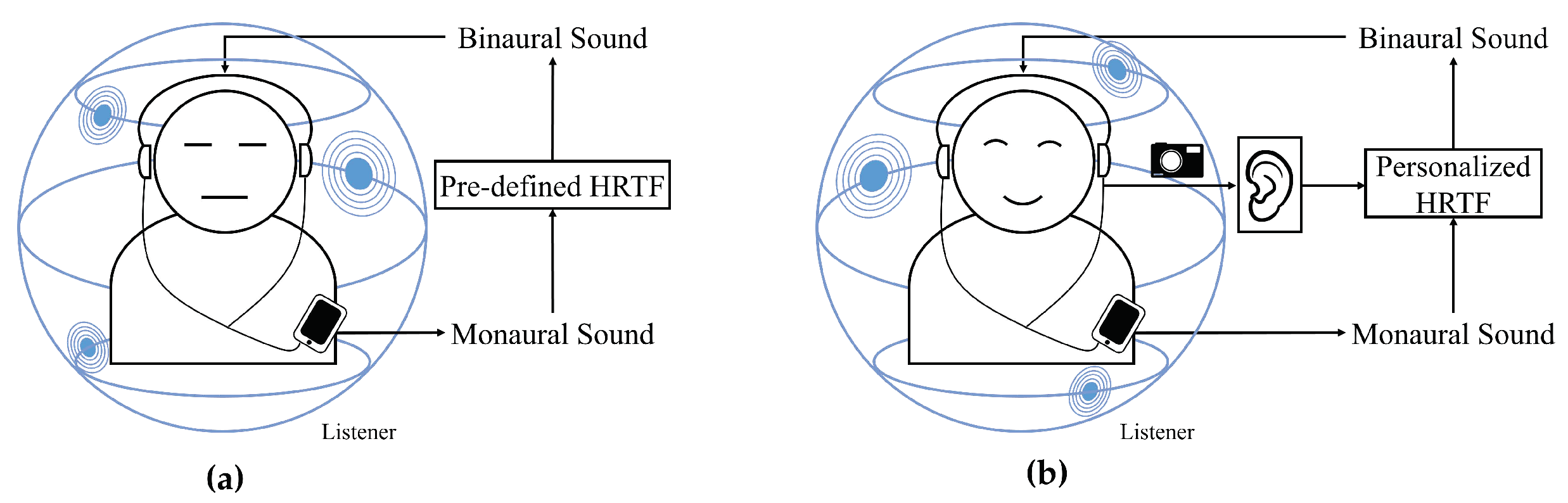Figure 1 shows a possible application of the personalized HRTF when playing sound in a binaural configuration. As shown in Figure 1a, a traditional approach to generating binaural sound from monaural sound is using a pre-defined HRTF, but the proposed method shown in Figure 1b enables us to provide better sound quality to a listener with HRTF that is personalized to the listener.

As HRTFs vary according to anthropometric measurements, HRTFs have been designed using statistical methods to create standard human head models [5]. However, since HRTFs are sensitive to individual characteristics, the spatial sound generated by an average HRTF model cannot be expected to produce faultless effects [6]. Therefore, it is necessary to measure the HRTF that suits the individual, but the measurement cost and time pose difficulties. To overcome these shortcomings, mathematical design methods based on measured HRTFs have also been studied in Reference [7,8,9]. Recently, artificial neural networks have shown meaningful results in various applications, such as temperature estimation and control [10,11], machinery fault diagnosis [12,13], material property prediction [14,15], load forecasting [16], handwritten digit recognition [17], and wind-speed forecasting [18]. In particular, based on biometric information, breast cancer classification [19] and corneal power estimation [20] showed good performance. A deep learning approach has also been applied to explore the complex relationship between anthropometric measurements and HRTFs [21,22], where anthropometric measurements including detailed measurements of the head, shoulders, and ears were used as the input features for a deep neural network (DNN). However, the performance of this approach was limited because ear-related measurements were difficult to obtain in real life. Instead of directly measuring anthropometric pinna measurements, we proposed a feature extraction method for ear images using an auto-encoder based on a convolutional neural network (CNN) [23] where the bottleneck features were extracted to represent personalized anthropometric data.

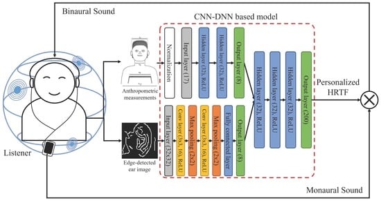
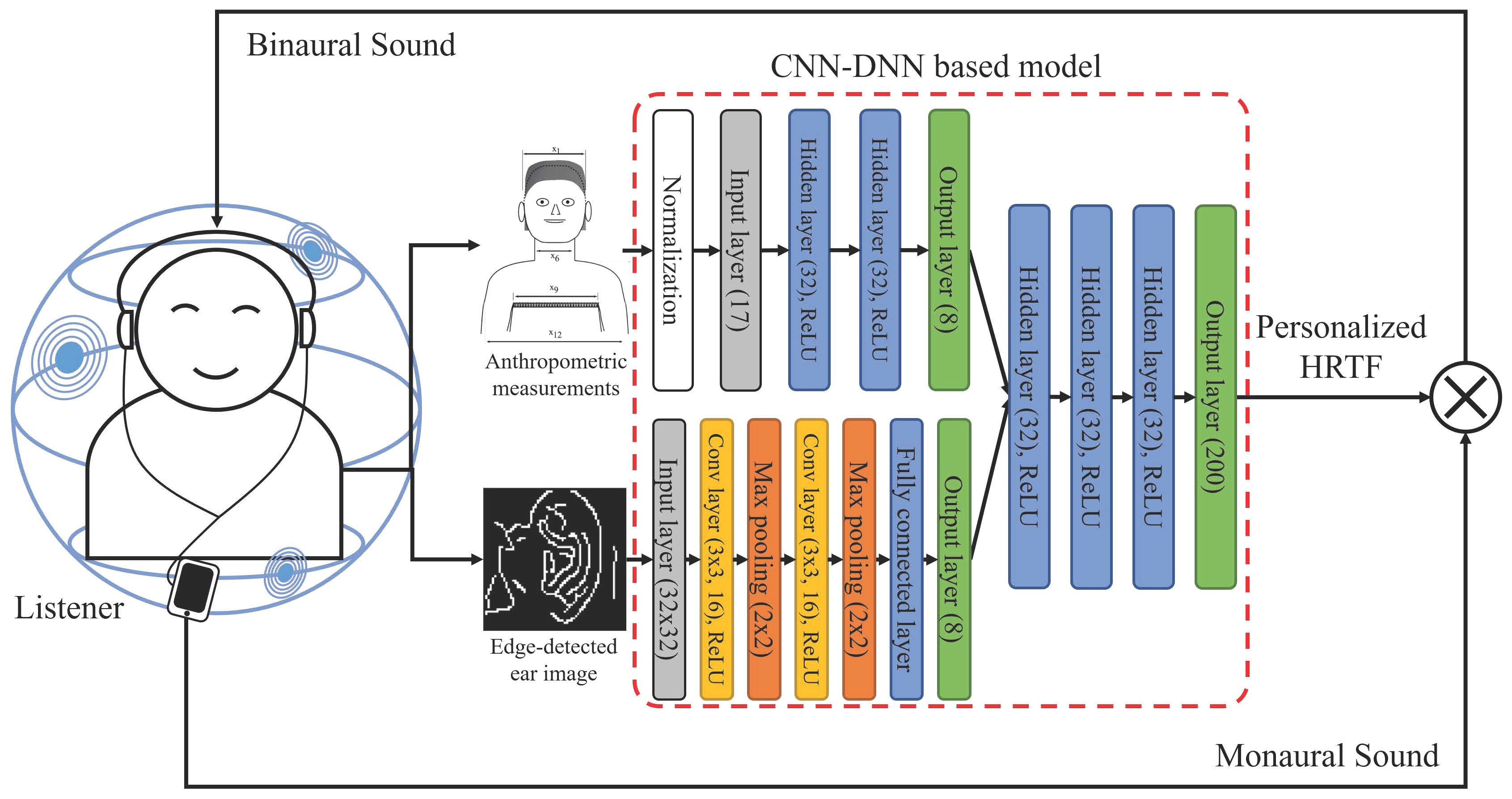
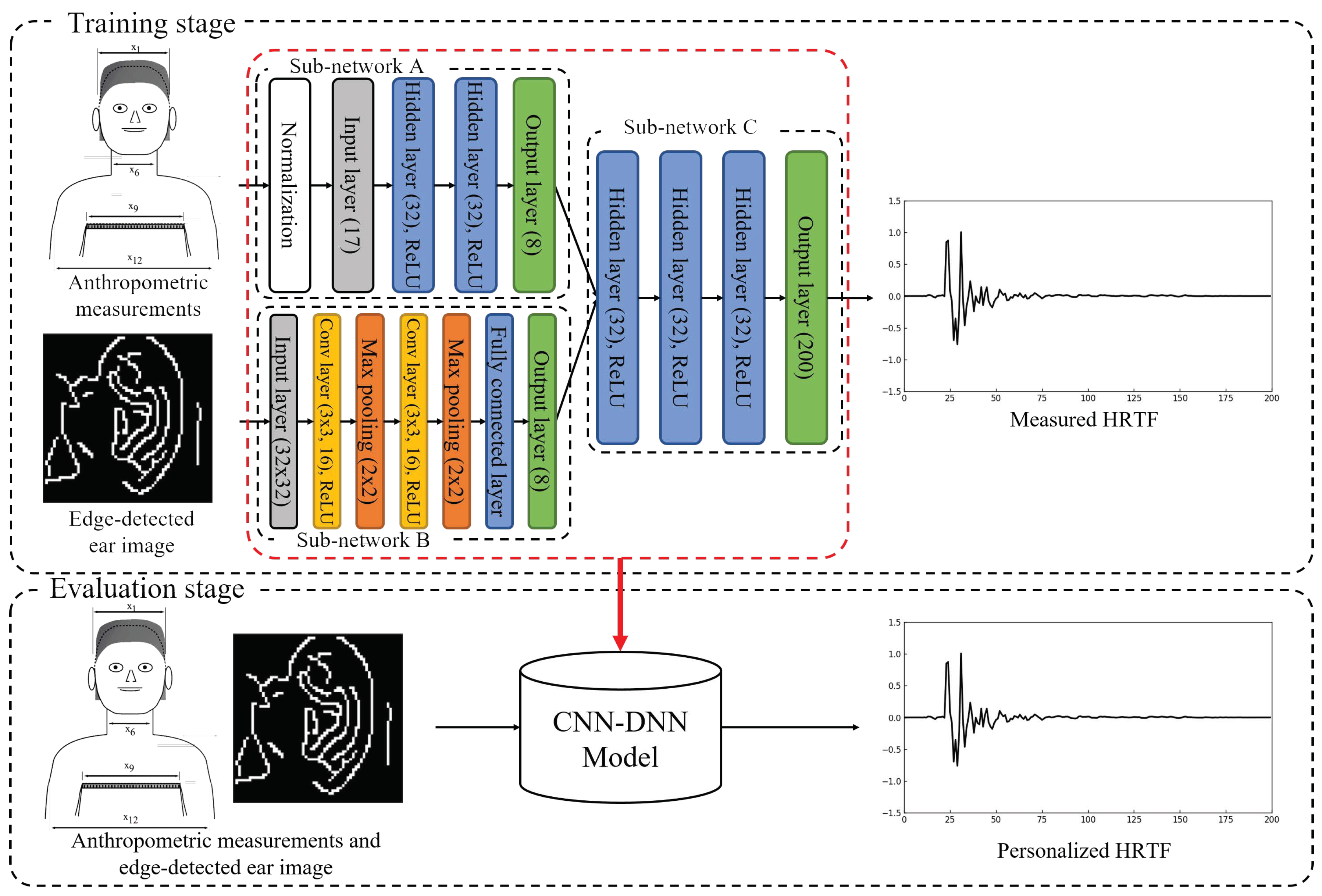
In this paper, our previous approach is extended to estimate a personalized HRTF using ear images instead of ear-related anthropometric measurements. 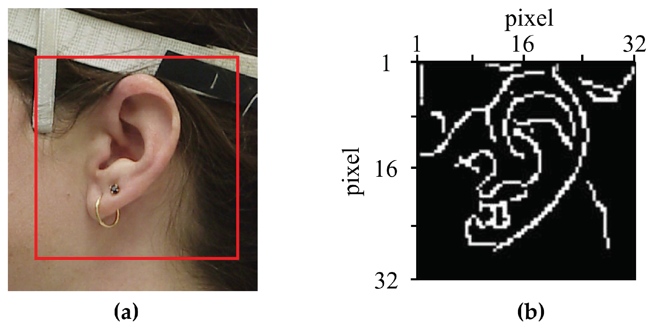The proposed neural network for the personalized HRTF estimation is composed of three sub-networks, the first of which is a feed-forward DNN that uses anthropometric measurements as input features to represent information on the relationship between anthropometric measurements and HRTFs [22]. The second sub-network tries to represent the personalized anthropometric measurements from ear images and is designed using a CNN, which enables us to obtain bottleneck features as proposed in Reference [23]. Lastly, the two different internal features obtained from the anthropometric measurements and ear images are combined using another DNN to estimate personalized HRTFs. The performance of the proposed method is evaluated objectively and subjectively. As objective measures, the root-mean-square error (RMSE) and log-spectral distortion (LSD) between the reference and estimated HRTF are calculated. In addition, the distance perceived by listeners after applying the estimated HRTF to a sound source is used as a subjective measure. Next, the performance of the proposed method is compared with that of HRTF estimation methods using the average [6] and estimated HRTF by a DNN trained with anthropometric measurements [22].

The remainder of this paper is organized as follows: Section 2 briefly reviews deep learning-based personalized HRTF estimation using whole anthropometric measurements. Section 3 proposes a personalized HRTF estimation method using a neural network that combines a DNN and a CNN in parallel applied to anthropometric measurements and ear images, respectively. Section 4 evaluates the performance of the proposed method and compares it with those of HRTF estimation methods using the average HRTF and the estimated HRTF by the DNN trained with anthropometric measurements. Finally, Section 5 concludes this paper.

2. Review of HRTF Modeling Using Anthropometrics

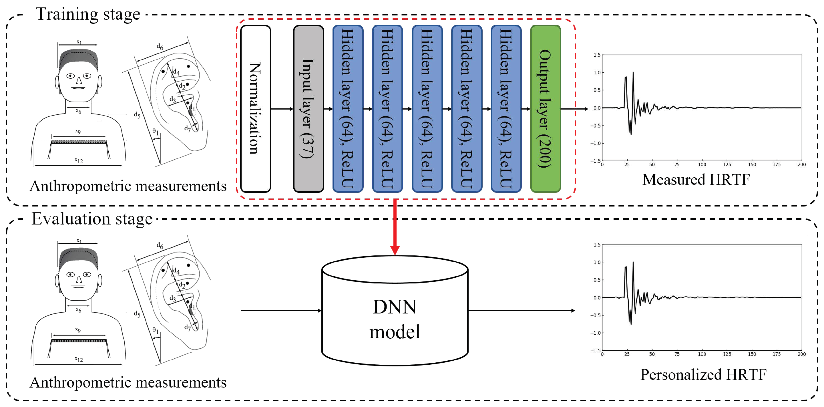
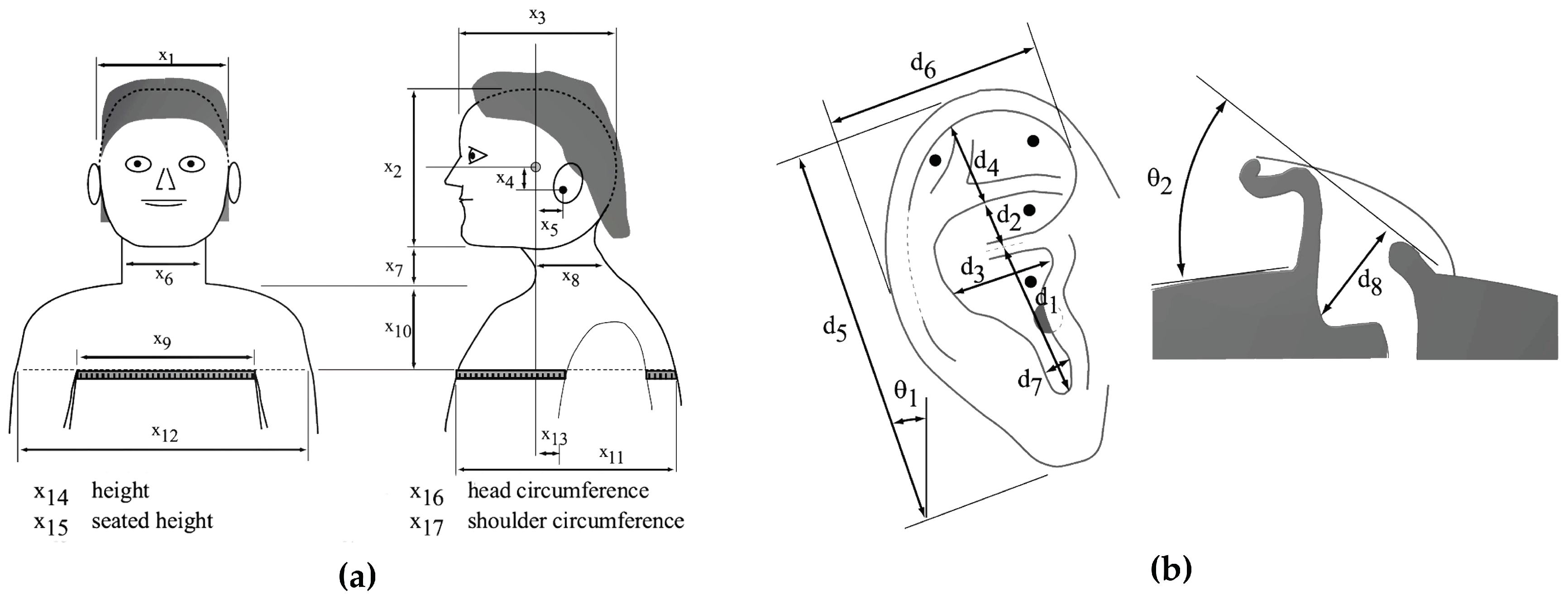
In this section, we briefly review a method for generating personalized HRTFs based on DNNs using anthropometric measurements, as shown in Figure 2 [22]. In the process of designing personalized HRTFs, the public HRTF database was provided by the Center for Image Processing and Integrated Computing (CIPIC) of the University of California at Davis [24]. This database included head-related impulse responses (HRIRs), another representation of HRTFs, for 45 subjects at 25 different azimuths and 50 different elevations with anthropometric measurements and ear images of each subject. The specifications of the anthropometric measurements included in the database are as shown in Figure 3 and

Table 1. List of anthropometric measurements in the Center for Image Processing and Integrated Computing (CIPIC) head-related transfer function (HRTF) database [24].

Variable	Measurement	Variable	Measurement	Variable	Measurement
$x_1$	Head width	$x_{10}$	Torso top height	$d_2$	Cymba concha height
$x_2$	Head height	$x_{11}$	Torso top depth	$d_3$	Cavum concha width
$x_3$	Head depth	$x_{12}$	Shoulder width	$d_4$	Fossa height
$x_4$	Pinna offset down	$x_{13}$	Head offset forward	$d_5$	Pinna height
$x_5$	Pinna offset back	$x_{14}$	Height	$d_6$	Pinna width
$x_6$	Neck width	$x_{15}$	Seated height	$d_7$	Integral incisure width
$x_7$	Neck height	$x_{16}$	Head circumference	$d_8$	Cavum concha depth
$x_8$	Neck depth	$x_{17}$	Shoulder circumference	${\theta }_1$	Pinna rotation angle
$x_9$	Torso top width	$d_1$	Cavum concha height	${\theta }_2$	Pinna flare angle

. In the CIPIC database, there were 17 parameters for head and torso measurements and 10 for pinna measurements. In particular, elevation and azimuth were sampled using a head-centered polar coordinate system. The elevations were uniformly sampled at intervals of 5.625° from −45° to 230.625° while the azimuths were sampled at 25 different angles from −80° to 80° with different steps of 5° to 15°. There were 1250 HRTFs of length 200 samples, corresponding to a duration of approximately 4.5 msec at a sampling rate of 44.1 kHz.

To compare the performance of our proposed method in Section 3 with the neural network model described in this section, a DNN is constructed as shown at the upper block of Figure 2. The DNN model here is composed of one input layer, five hidden layers, and one output layer. There are 37 input units (17 parameters for the height and circumference measurements and 20 for the pinna measurements for both ears), as described in Table 1, and the number of output nodes is set to 200, corresponding to the length of the HRTFs. In addition, the number of each hidden layer’s nodes is set to 64 and the rectified linear unit (ReLU) is applied as an activation function for each layer because the ReLU activation function is known to be effective for solving gradient-vanishing problems [25]. Moreover, since the range of anthropometric measurement is different between measurements, a measurement with a small range may not influence learning. Thus, each input feature for the DNN is normalized using the mean and variance for all training data without regard for the subjects, such as

$${\overline{z}}_i={\left(1+e^{-\frac{\left(z_i-{\mu }_i\right)}{{\sigma }_i}}\right)}^{-1}$$

(1)

where $z_i$ and ${\overline{z}}_i$ are the i-th component of the input and normalized feature vector, respectively, and ${\mu }_i$ and ${\sigma }_i$ are the mean and standard deviation of all the training data, respectively. Note that $z_i$ could be $x_i, d_i,$ or ${\theta }_i$ in Table 1.

For training the DNN, Xavier initialization is utilized for the initial weights of the configured model, and the biases are initialized at zero [26]. The mean square error (MSE) between the original target and the estimate target is selected as a cost function [27]. The adaptive moment estimation (Adam) optimization is utilized for the backpropagation algorithm and the first- and second-moment decay rates are set to 0.9 and 0.999, respectively, with a learning rate of 0.001 [28]. In addition, the dropout technique is utilized with the keep probability of 0.9 [29]. Finally, the model was trained for 20,000 epochs. The performance of the DNN described thus far will be discussed in Section 4.

3. Proposed Personalized HRTF Estimation Method

3.1. Neural Network Architecture

This section proposes a method for estimating the personalized HRTF using ear images and anthropometric measurements. Since the measured anthropometric data may potentially be missing information that may have been used to estimate HRTFs, it is difficult to take the ear measurements represented in Figure 3b in practice. Thus, instead of measuring the anthropometric parameters of a physical ear, the proposed method directly uses an image of the ear.

Figure 4 illustrates a block diagram of the proposed HRTF personalized method, including the architecture of a DNN for the proposed personalized HRTF estimation, where both anthropometric measurements and ear images are used as input features, and HRTFs are used as target features. As shown in the figure, the proposed neural network is composed of three sub-networks. The first sub-network of the proposed neural network is a DNN that uses anthropometric measurements as input features to represent the information on the relationship between anthropometric measurements and HRTFs, which is referred to as “Sub-network A”. The second sub-network is a feature representation network based on CNN from ear images and referred to as “Sub-network B”. The two sub-networks are combined together using another DNN to estimate personalized HRTFs, referred to as “Sub-network C”.

Sub-network A is composed of an input layer, two hidden layers, and an output layer, as illustrated in the left-upper corner in Figure 4. Compared to the input features of the DNN in Section 2, only 17 features (height and circumference measurements) are used here as input features for Sub-network A. The pinna measurements of both ears can be modeled by Sub-network B, as will be described in the next paragraph. In addition, the number of each hidden layer’s nodes is set to 32, and the output layer consists of eight nodes and becomes a part of the input layer for Sub-network C. As an activation function, the ReLU is applied to the hidden layers and the output layer.

Sub-network B is composed of an input layer, two convolution layers, two max-pooling layers, a fully connected layer, and an output layer. The 32 × 32 edge-detected ear images are used for the input features of this sub-network. A detailed explanation is given in Section 3.2. Each convolution layer consists of 3 × 3 kernels where the number of the kernels is 16. The max-pooling layer is followed by each convolution layer of 2 × 2 size. A fully connected layer converts a 2-D shape output to a 1-D shape from the last max-pooling layer. The output layer of Sub-network B consists of eight nodes and is also used as a part of the input layer of Sub-network C. Similar to Sub-network A, the ReLU activation function is applied for two convolution layers, the fully connected layer, and the output layer.

Lastly, Sub-network C consists of an integrated input layer with 16 nodes and three hidden layers with 32 nodes each. The output layer has 200 nodes that correspond to the length of HRTFs in the CIPIC database, as described in Section 2. In addition, the ReLU activation function is applied for both the hidden layers and the output layer.

3.2. Extraction of Ear Images

The ear images in the CIPIC database have different resolutions. Thus, a 32 × 32 region of interest (ROI) is applied to each image in this paper because image processing for the ear image requires a consistent resolution. Moreover, color ear images are converted to grayscale ones because skin color has no impact on sound propagation.

In general, the more complex a neural network model is, the more data it requires; furthermore, the use of insufficient data can cause severe performance degradation due to the overfitting problem. In particular, this problem occurs more frequently in regression models [30]. For example, the National Institute of Standards and Technology (MNIST) challenge, which recognizes handwritten digits, provides 60,000 training images, and 10,000 test images [31]. Meanwhile, only 31 ear images are included in the CIPIC database, and such insufficient data can lead to an overfitting problem. Thus, instead of using features extracted from the images, edge-detected images are directly used as the input features of Sub-network B. Therefore, the first layer of CNN performs filtering to extract low-level features, such as edges and lines.

Figure 5 illustrates an example of an original color image from the CIPIC database as well as the edge-detected ear image. The image size of the edge-detected ear image, as shown in Figure 5b, is 32 × 32 pixels, where the ear image corresponds to the boxed area of Figure 5a. The Canny edge detection algorithm [32] is used here, which is as follows:

(1)

Apply a Gaussian filter to the image to remove noise and unwanted details

(2)

Find the intensity gradients of the image

(3)

Apply non-maximum suppression to remove spurious responses to edge detection

(4)

Apply double thresholds with hysteresis by suppressing all edges that are weak and not connected to a strong edge.

3.3. Supervised Learning

The training procedure for the proposed neural network is similar to that described in Section 2. In the training phase, well-initialized weights can lead to good results, such as low initial cost or fast convergence [33]. To initialize all weights of layers, we use the Xavier initialization technique, while all biases are initialized as zero [26]. An MSE between the reference target and the estimated one is applied with a back-propagation algorithm [27]. A basic gradient descent algorithm based on the back-propagation method is used to update weights by minimizing the cost. In this process, the Adam optimization technique that uses momentum and gradient adaptation methods is applied with the first and second moment decay rates of 0.9 and 0.999, respectively, and the learning rate is set to 0.0001 [28]. To increase the convergence speed and prevent overfitting problems, a dropout technique is applied with a keep probability of 0.5, and a data augmentation technique of adding additive white Gaussian noise (AWGN) is applied with a value of 0.3 [29,34]. Finally, the configured model is trained for 100,000 epochs.

4. Performance Evaluation

In this section, the performance of the proposed personalized HRTF estimation method was evaluated in terms of both objective and subjective tests. For objective tests, the RMSE and LSD between the reference and estimated HRTF were measured. For the subjective test, a sound localization experiment was performed, and the distance perceived by listeners after applying the estimated HRTF to a sound source was measured. Subsequently, the performance of the proposed method was compared to those of the following other HRTF estimation methods: (1) an HRTF estimation method using average HRTF, referred to as “Average HRTF”; (2) the estimated HRTF by a DNN trained with anthropometric measurements in Section 2 [11], referred to as “DNN(37) HRTF” because there were 37 anthropometric measurements including ear measurements; (3) the estimated HRTF by a DNN trained with only 17 head and torso measurements, referred to as “DNN(17) HRTF.” Henceforth, the proposed method is referred to as “CNN–DNN HRTF.” Note that since it was difficult to obtain anthropometric measurements of the pinna for a test subject, the performance of the DNN in Section 2 was only evaluated using objective measures.

All methods were implemented in MATLAB with a version of R2013b using Tensorflow whose version was r1.1.0 with Python 3.5.2. In this paper, 30 subjects and one subject of the CIPIC database were used for training and testing each neural network, respectively. Then, 31 cross-validations were performed and measurements were averaged over all cross-validations. Note here that the average HRTF method took an average over the HRTFs of all 31 subjects. In addition, since there were 1250 different environments (25 azimuths and 50 elevations), both the proposed method and the DNN-based methods were constructed in each different environment, resulting in 1250 CNN–DNN HRTFs, 1250 DNN(37) HRTFs, and 1250 DNN(17) HRTFs.

4.1. Objective Evaluation

As mentioned earlier, there were two objectives measured here. One was the RMSE between the reference HRTF $y\left(n\right)$ and the estimated HRTF $\widehat{y}\left(n\right),$ which was defined as

$$\mathrm{RMSE}\left(\mathrm{y},\widehat{y}\right)=20{\log }_{10}\sqrt{\frac{1}{N}{\displaystyle \sum }_{n=0}^{N-1}{\left(y\left(n\right)-\widehat{y}\left(n\right)\right)}^2}$$

(2)

where N (=200) was the total length of the HRTF. In addition, the LSD was defined as

$$\mathrm{LSD}\left(Y, \widehat{Y}\right)=\sqrt{\frac{1}{M}{\displaystyle \sum }_{k=0}^M{\left(20{\log }_{10}\frac{\left|Y\left(k\right)\right|}{\left|\widehat{Y}\left(k\right)\right|}\right)}^2}$$

(3)

where $Y\left(k\right)$ and $\widehat{Y}\left(k\right)$ were obtained by applying a fast Fourier transform (FFT) to $\mathrm{y}\left(n\right)$ and $\widehat{y}\left(n\right)$, respectively, and M (=512) was half the size of the FFT.

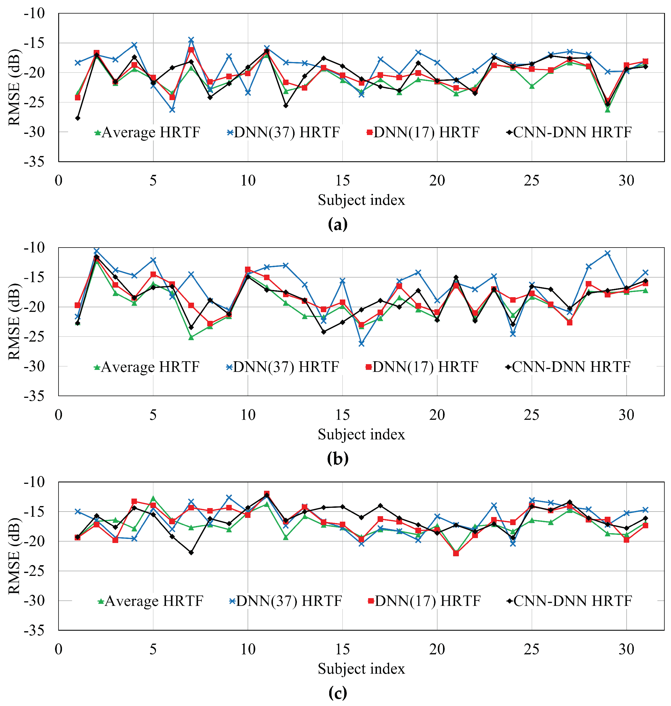
Figure 6 compares the RMSEs of the individual subject according to different HRTF estimation methods, measured at −135°, −80°, and −45°. Note that the performances of the HRTFs at 135°, 80°, and 45° were identical to those at −135°, −80°, and −45°, respectively. In addition,

Table 2. Comparison of the average root mean square errors (RMSEs) of different HRTF estimation methods at −135°, −80°, and −45°.

Azimuth	Average HRTF	DNN(37) HRTF	DNN(17) HRTF	CNN–DNN HRTF
−135°	−20.98	−18.94	−20.31	−20.26
−80°	−19.39	−16.78	−18.29	−18.60
−45°	−17.32	−16.25	−16.53	−16.35
Avg.	−19.23	−17.32	−18.38	−18.40

compares the average HRTF over all the HRTFs in the CIPIC database, measured at −135°, −80°, and −45°. As shown in Figure 6 and Table 2, the DNN-based method (DNN(37) HRTF) and the proposed method provided RMSEs that were 1.91 and 0.88 dB higher than the average HRTF method, respectively. Even though the average HRTF had the lowest RMSE because this was obtained from exact pinna measurements, it was actually hard to get pinna measurement data from live human ears. Without such pinna measurements, the DNN-based method increased RMSE by 0.02 dB. Thus, the RMSE of the estimated HRTF by the proposed method was lowered than that estimated by the DNN(17) HRTF.

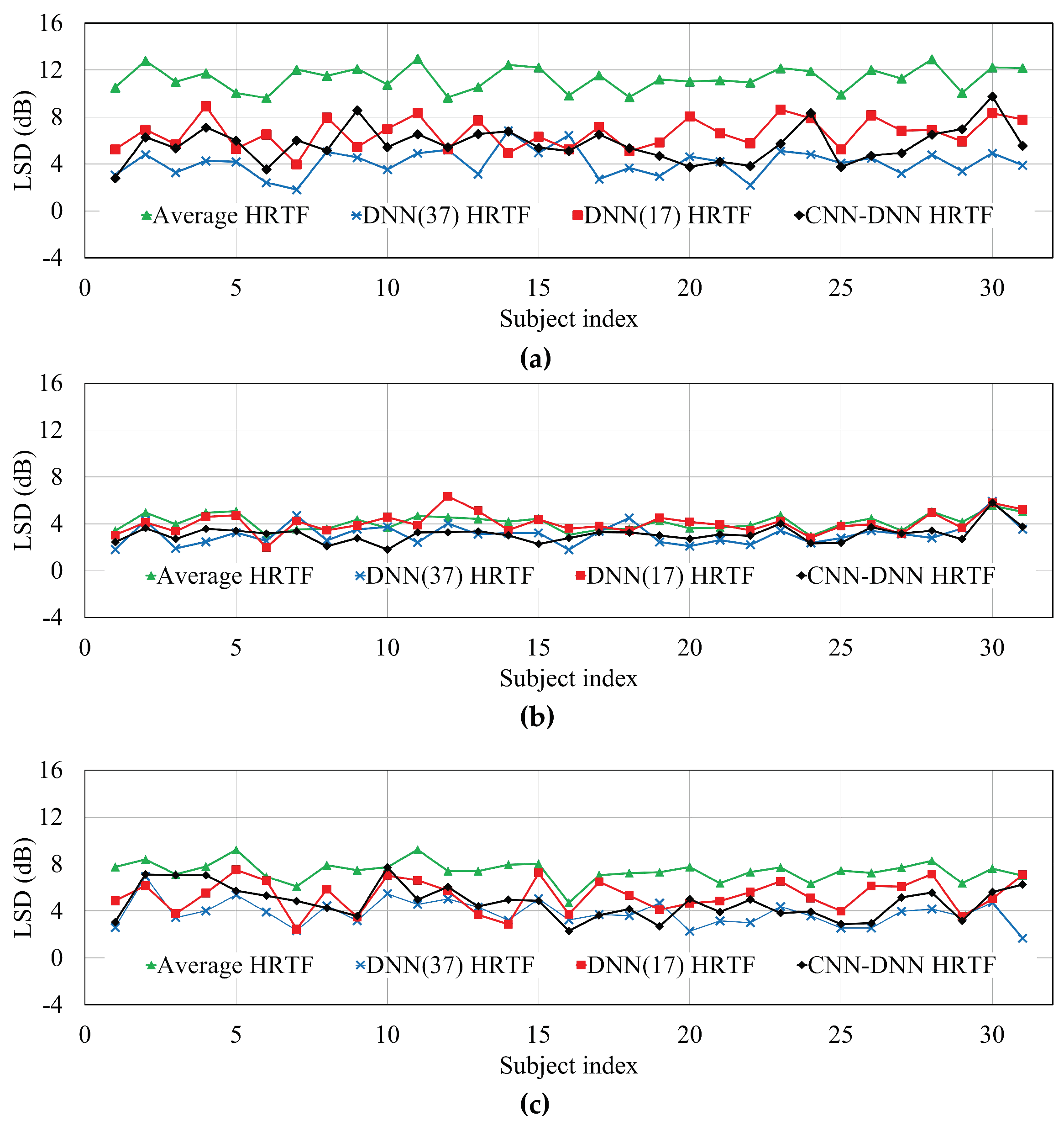
Next, the LSD was computed between the reference HRTF and its estimated HRTF for each of the four different HRTF estimation methods. Figure 7 and

Table 3. Comparison of the average log spectral distances (LSDs) for different HRTF estimation methods at −135°, −80°, and −45°.

Azimuth	Average HRTF	DNN(37) HRTF	DNN(17) HRTF	CNN–DNN HRTF
−135°	11.29	4.12	6.62	5.70
−80°	4.12	3.12	4.05	3.11
−45°	7.41	3.82	5.30	4.61
Avg.	7.61	3.69	5.32	4.47

compare the LSDs of the individual subject and the average LSD according to different HRTF estimation methods, measured at −135°, −80°, and −45°, respectively. As shown in the figure and table, the average LSD measured from the DNN(37) HRTFs was lowest among the methods. However, similar to the RMSE described above, the average LSD of the HRTFs estimated by the proposed method was lower by 0.85 dB compared to that by DNN(17) HRTFs. In particular, the LSDs for the HRTFs estimated by both neural network-based methods were greatly reduced compared to the average HRTF method.

4.2. Subjective Evaluation

In this subsection, we carried out a subjective evaluation of the localization experiment in which five listeners (three males and two females) without any auditory disease participated. This experiment was performed using Microsoft Surface Pro 4, which was manufactured by Pegatron Corporation, Taipei, Taiwan, with Sennheiser HD 650 headphones.

Table 4. Measured anthropometric data of five listeners.

	Variable (cm)	${\mathit{x}}_{\mathbf{1}}$	${\mathit{x}}_{\mathbf{2}}$	${\mathit{x}}_{\mathbf{3}}$	${\mathit{x}}_{\mathbf{4}}$	${\mathit{x}}_{\mathbf{5}}$	${\mathit{x}}_{\mathbf{6}}$	${\mathit{x}}_{\mathbf{7}}$	${\mathit{x}}_{\mathbf{8}}$	${\mathit{x}}_{\mathbf{9}}$
Listener
M1		17.8	23.7	18.8	1.8	4.0	11.4	9.2	10.9	33.1
M2		16.8	25.1	19.6	2.5	3.4	11.7	7.4	11.7	42.2
M3		17.6	23.4	18.2	2.8	4.7	12.4	8.4	13.4	34.6
F1		13.4	21.5	17.3	2.3	2.6	8.4	4.5	8.7	26.3
F2		14.6	21.3	17.6	2.2	2.7	9.7	5.2	9.2	37.3
	Variable (cm)	${\mathit{x}}_{\mathbf{10}}$	${\mathit{x}}_{\mathbf{11}}$	${\mathit{x}}_{\mathbf{12}}$	${\mathit{x}}_{\mathbf{13}}$	${\mathit{x}}_{\mathbf{14}}$	${\mathit{x}}_{\mathbf{15}}$	${\mathit{x}}_{\mathbf{16}}$	${\mathit{x}}_{\mathbf{17}}$
Listener
M1		15.3	21.7	45.3	3.4	183.5	96.0	60.0	113.6
M2		12.6	22.7	52.1	1.4	184.2	90.0	62.4	130.4
M3		13.8	25.9	49.8	1.3	175.1	89.5	61.0	123.3
F1		9.6	78.9	38.7	2.0	161.0	80.3	58.0	90.4
F2		7.8	28.0	44.7	2.2	160.2	77.2	55.5	106.0

shows the anthropometric measurements of each listener, where male and female listeners are denoted as M1–3 and F1–2, respectively, and $x_1–x_{17}$ are head and torso measurements, as described in Table 1. Both these anthropometric measurements and each listener’s ear images were used as input features for the proposed method. Then, each personalized HRTF was estimated in an environment for each specific listener by the proposed method and the DNN-based method using only head and torso measurements. Next, the estimated HRTFs and average HRTF at a given environment were applied to a speech signal of 10-s duration at a sampling rate of 44.1 kHz. In other words, each HRTF was convoluted with the speech signal. Here, the environments selected in this paper were at eight different azimuths (0°, ±45°, ±80°, ±135°, and 180°) with an elevation of 0°. For the evaluation, each participant listened to a pair of speech signals that were convolved with average HRTF, DNN(17) HRTF, or CNN–DNN HRTF, and then he/she judged the azimuth at which each speech signal was assumed to be directed.

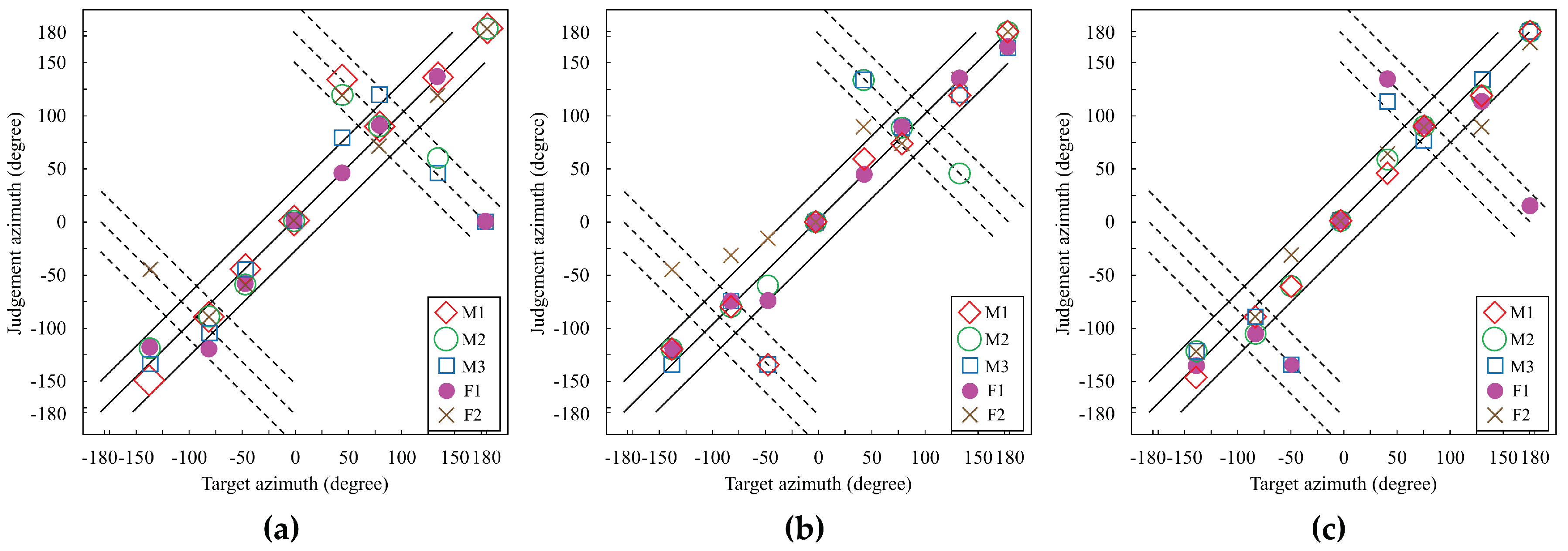
Figure 8 illustrates the sound localization performance to show the azimuths judged by the participants versus the target azimuth when average HRTF, DNN(17) HRTF, and CNN–DNN HRTF were used. In the figure, the main diagonal solid line indicates correct judgment, and the upper and lower off-diagonal solid lines indicate ±30° margin of error. On the one hand, if a sound is judged on or near the dashed lines, this corresponds to front/back confusion. For example, when the target azimuth was set to 50°, the sound should be located in the front-right direction. However, the sound seemed to be heard in the back-right direction if the azimuth was judged at 130°. In addition, two dotted lines parallel to the dashed lines means that the margins of errors are ±30°. As shown in the figure, judged azimuths when using the proposed method were clustered better than when using average HRTFs or DNN(17) HRTFs.

Table 5. Comparison of average accuracies within specific margins (15° and 30°) and front/back confusion rate for different HRTF estimation methods.

	Average HRTF	DNN(17) HRTF	CNN–DNN HRTF
Accuracy within ±15° (%)	70.0	70.0	80.0
Accuracy within ±30° (%)	72.5	82.5	85.0
Front/back confusion rate (%)	25.0	15.0	12.5

compares the accuracies within specific margins, such as ±15° and ±30°, and the front/back confusion rate of the localization experiment between the average HRTF and the proposed method. As shown in the table, the proposed CNN–DNN-based HRTF estimation method achieved higher accuracies of 10% and 12.5% than the average HRTF method for the ±15° and ±30° margins, respectively. In addition, the accuracy of the proposed method was improved by 10% and 2.5%, compared to the average HRTF method and the DNN(17)-based method, respectively. Moreover, the front/back confusion rate of the proposed method was reduced by 12.5% and 2.5%, compared to the average HRTF method and the DNN(17)-based method, respectively.

4.3. Performance Comparison with Data Augmentation

The number of ear images in the CIPIC database seems so small that the deep learning model could be overfitted to the training data [30]. Data augmentation can be an alternative to prevent this problem. In this paper, data augmentation techniques, such as zero-phase component analysis (ZCA) [35] and/or image shifting [36], were applied to 30 ear images; thus, the total numbers of training data were increased to 60 after applying ZCA and 90 after applying ZCA combined with image shifting, respectively.

Table 6. Comparison of average RMSEs of the proposed HRTF estimation method with/without data augmentation at −135°, −80°, and −45°.

Azimuth	CNN–DNN HRTF	CNN–DNN HRTF with ZCA	CNN–DNN HRTF with ZCA + Image Shift
−135°	−20.26	−20.20	−19.44
−80°	−18.60	−18.60	−18.49
−45°	−16.35	−16.16	−15.93
Avg.	−18.40	−18.32	−17.95

and

Table 7. Comparison of average LSDs for the proposed HRTF estimation method with/without data augmentation at −135°, −80°, and −45°.

Azimuth	CNN–DNN HRTF	CNN–DNN HRTF with ZCA	CNN–DNN HRTF with ZCA + Image Shift
−135°	5.70	5.43	5.27
−80°	3.11	3.30	3.26
−45°	4.61	4.27	4.01
Avg.	4.47	4.33	4.18

compare the RMSEs and LSDs for individual subjects according to the proposed HRTF estimation method with and without data augmentation, respectively, as measured at −135°, −80°, and −45°. As shown in Table 6, the average RMSE went a little higher as the amount of augmentation data increased. In other words, the average RMSE of ZCA + Image Shift-CNN–DNN HRTF was increased by 0.45 dB compared to that of CNN–DNN HRTF. Meanwhile, the average LSD was decreased as the amount of data augmentation increased. Table 7 showed that the ZCA+Image Shift-CNN–DNN HRTF could reduce the average LSD by 0.29 dB compared to CNN–DNN HRTF.

5. Conclusions

In this paper, a personalized HRTF estimation method has been proposed on the basis of deep neural networks using anthropometric measurements and ear images. In particular, while a conventional DNN-based method aimed to estimate HRTFs using the anthropometric data including head, torso, and pinna measurements, the proposed method replaced pinna measurements with ear images due to the difficulty of obtaining pinna measurements for live human ears. Thus, the neural network in the proposed method was composed of three sub-networks. The first one was a DNN to represent the head and torso measurements and the second one was a CNN for extracting pinna measurements from edge-detected ear images instead of actually measured pinna data. The two sub-networks were then merged into another DNN to estimate a personalized HRTF.

The performance of the proposed personalized HRTF estimation method was evaluated in terms of both objective and subjective tests. For the objective tests, the RMSEs and LSDs between the reference and estimated HRTFs were measured. For the subjective test, a sound localization experiment was performed, and the distance perceived by listeners after applying the estimated HRTF to a sound source was measured. After that, the performance of the proposed method was compared with those of HRTF estimation methods using average HRTF, the estimated HRTF by a DNN trained with anthropometric measurements, and the estimated HRTF by a DNN trained with only head and torso measurements. Consequently, it was shown from the objective evaluation that the proposed method decreased the RMSE and LSD by 0.02 and 0.85 dB, respectively, compared to the DNN-based method using anthropometric data without pinna measurements. In addition, it was shown form the subjective evaluation that the proposed method provided higher localization accuracy of 6% than the DNN-based method. In addition, the front/back confusion rate for the proposed method was reduced by 2.5% compared to the DNN-based method. Next, data augmentation was performed to increase the training data by applying zero-phase component analysis (ZCA) and image shifting. Thus, it was shown that after data augmentation, the proposed method could increase the RMSE but reduce the LSD by 0.29 dB, compared to only using ear images from the CIPIC HRTF database.

In future work, to improve the performance of the proposed CNN–DNN HRTF estimation method, different model structures need to be studied, such as a residual network [37] or a dense network [38]. Moreover, the CIPIC HRTF database is too small to train deep learning models. Even though data augmentation has been performed in this paper, further sophisticated investigation of the effect of data augmentation on the performance of the proposed method, particularly the RMSE, will be studied.

References

1. Rumsey, F. Spatial Audio; Focal Press: Woburn, MA, USA, 2001. [Google Scholar]
2. Blauert, J. Spatial Hearing: The Psychophysics of Human Sound Localization; MIT Press: Cambridge, MA, USA, 1997. [Google Scholar]
3. Roffler, S.K.; Butler, R.A. Factors that influence the localization of sound in the vertical plane. J. Acoust. Soc. Am. 1968, 43, 1255–1259. [Google Scholar] [CrossRef] [PubMed]
4. Bronkhorst, A.W.; Houtgas, T. Auditory distance perception in rooms. Nature 1994, 397, 517–520. [Google Scholar] [CrossRef] [PubMed]
5. Begault, R.D. 3D Sound for Virtual Reality and Multimedia; Academic Press: Cambridge, MA, USA, 1994. [Google Scholar]
6. Wenzel, E.M.; Arruda, M.; Kistler, D.J.; Wightman, F.L. Localization using nonindividualized head-related transfer functions. J. Acoust. Soc. Am. 1993, 94, 111–123. [Google Scholar] [CrossRef] [PubMed]
7. Brown, C.P.; Duda, R.O. An efficient HRTF model for 3-D sound. In Proceedings of the IEEE Workshop on Applications of Signal Processing to Audio and Acoustics, New Paltz, NY, USA, 19–22 October 1997; pp. 298–301. [Google Scholar]
8. Kistler, D.J.; Wightman, F.L. A model of head-related transfer functions based on principal components analysis and minimum-phase reconstruction. J. Acoust. Soc. Am. 1992, 91, 1637–1647. [Google Scholar] [CrossRef] [PubMed]
9. Cheung, N.-M.; Trautman, S.; Horner, A. Head-related transfer function modeling in 3-D sound systems with genetic algorithms. J. Audio Eng. Soc. 1998, 46, 531–539. [Google Scholar]
10. Kochan, O.; Sapojnyk, H.; Kochan, R. Temperature field control method based on neural network. In Proceedings of the IEEE 7th International Conference on Intelligent Data Acquisition and Advanced Computing Systems, Berlin, Germany, 12–14 September 2013; pp. 21–24. [Google Scholar]
11. Zhengbing, H.; Jotsov, V.; Jun, S.; Kochan, O.; Mykyichuk, M.; Kochan, R.; Sasiuk, T. Data science applications to improve accuracy of thermocouples. In Proceedings of the IEEE 8th International Conference on Intelligent Systems, Sofia, Bulgaria, 4–6 September 2016; pp. 180–188. [Google Scholar]
12. Jia, F.; Lei, Y.; Lu, N.; Xing, S. Deep normalized convolutional neural network for imbalanced fault classification of machinery and its understanding via visualization. Mech. Syst. Signal Process. 2018, 110, 349–367. [Google Scholar] [CrossRef]
13. Gajewski, J.; Vališ, D. The determination of combustion engine condition and reliability using oil analysis by MLP and RBF neural networks. Tribol. Int. 2017, 115, 557–572. [Google Scholar] [CrossRef]
14. Wilk-Kolodziejczyk, D.; Regulski, K.; Gumienny, G.; Kacprzyk, B.; Kluska-Nawarecka, S.; Jaskowiec, K. Data mining tools in identifying the components of the microstructure of compacted graphite iron based on the content of alloying elements. Int. J. Adv. Manuf. Technol. 2018, 95, 3127–3139. [Google Scholar] [CrossRef]
15. Ganovska, B.; Molitoris, M.; Hosovsky, A.; Pitel, J.; Krolczyk, J.B.; Ruggierio, A.; Krolczyk, G.M.; Hloch, S. Design of the model for the on-line control of the AWJ technology based on neural networks. Indian J. Eng. Mater. Sci. 2016, 23, 279–287. [Google Scholar]
16. Li, Y.; Huang, Y.; Zhang, M. Short-term load forecasting for electric vehicle charging station based on niche immunity lion algorithm and convolutional neural network. Energies 2018, 11, 1253. [Google Scholar] [CrossRef]
17. Alani, A.A. Arabic handwritten digit recognition based on restricted Boltzmann machine and convolutional neural networks. Information 2017, 8, 142. [Google Scholar] [CrossRef]
18. Huang, C.-J.; Kuo, P.-H. A short-term wind speed forecasting model by using artificial neural networks with stochastic optimization for renewable energy systems. Energies 2018, 11, 2777. [Google Scholar] [CrossRef]
19. Nahid, A.-A.; Kong, Y. Histopathological breast-image classification using local and frequency domains by convolutional neural network. Information 2018, 9, 19. [Google Scholar] [CrossRef]
20. Koprowski, R.; Lanza, M.; Irregolare, C. Corneal power evaluation after myopic corneal refractive surgery using artificial neural networks. Biomed. Eng. Online 2016, 15, 121. [Google Scholar] [CrossRef] [PubMed]
21. Hu, H.; Zhou, L.; Ma, H.; Wu, Z. HRTF personalization based on artificial neural network in individual virtual auditory space. Appl. Acoust. 2008, 69, 163–172. [Google Scholar] [CrossRef]
22. Chun, C.J.; Moon, J.M.; Lee, G.W.; Kim, N.K.; Kim, H.K. Deep neural network based HRTF personalization using anthropometric measurements. In Proceedings of the 143rd AES Convention, New York, NY, USA, 18–21 October 2017. Preprint 9860. [Google Scholar]
23. Lee, G.W.; Moon, J.M.; Chun, C.J.; Kim, H.K. On the use of bottleneck features of CNN auto-encoder for personalized HRTFs. In Proceedings of the 144th AES Convention, Milan, Italy, 23–26 May 2018. Preprint 10023. [Google Scholar]
24. Algazi, V.R.; Duda, R.O.; Thompson, D.M.; Avendano, C. The CIPIC HRTF database. In Proceedings of the IEEE Workshop on Applications of Signal Processing to Audio and Acoustics, New Paltz, NY, USA, 21–24 October 2001; pp. 99–102. [Google Scholar]
25. Glorot, X.; Bordes, A.; Bengio, Y. Deep sparse rectifier neural networks. Proceeding of the 14th International Conference on Artificial Intelligence and Statistics, Fort Lauderdale, FL, USA, 11–13 April 2011; pp. 315–323. [Google Scholar]
26. Glorot, X.; Bengio, Y. Understanding the difficulty of training deep feedforward neural networks. In Proceedings of the 13th International Conference on Artificial Intelligence and Statistics, Sardinia, Italy, 13–15 May 2010; pp. 249–256. [Google Scholar]
27. Rumelhart, D.E.; Hinton, G.E.; Williams, R.J. Learning representations by back-propagating errors. Nature 1986, 323, 533–536. [Google Scholar] [CrossRef]
28. Kingma, D.P.; Ba, J.L. ADAM: A method for stochastic optimization. In Proceedings of the 3rd International Conference on Learning Representations, San Diego, CA, USA, 7–9 May 2015; pp. 1–15. [Google Scholar]
29. Srivastava, N.; Hinton, G.; Krizhevsky, A.; Sutskever, I.; Salakhutdinov, R. Dropout: A simple way to prevent neural networks from overfitting. J. Mach. Learn. Res. 2014, 15, 1929–1958. [Google Scholar]
30. Frank, E.H., Jr. Regression Modeling Strategies; Springer: Berlin/Heidelberg, Germany, 2006. [Google Scholar]
31. LeCun, Y.; Cortes, C. MNIST Handwritten Digit Database. Available online: http://yann.lecun.com/exdb/mnist/ (accessed on 28 September 2018).
32. Canny, J. A computational approach to edge detection. IEEE Trans. Pattern Anal. Mach. Intell. 1986, 8, 679–698. [Google Scholar] [CrossRef] [PubMed]
33. Sutskever, I.; Martens, J.; Dahl, G.; Hinton, G. On the importance of initialization and momentum in deep learning. In Proceedings of the 30th International Conference on Machine Learning, Atlanta, GA, USA, 16–21 June 2013; pp. 1139–1147. [Google Scholar]
34. Audhkhasi, K.; Osoba, O.; Kosko, B. Noise-enhanced convolutional neural networks. Neural Netw. 2016, 78, 15–23. [Google Scholar] [CrossRef] [PubMed]
35. Krizhevsky, A.; Hinton, G. Learning Multiple Layers of Features from Tiny Images; Technical Report; University of Toronto: Toronto, ON, Canada, 2009. [Google Scholar]
36. Simard, P.Y.; Steinkraus, D.; Platt, J.C. Best practices for convolutional neural networks applied to visual document analysis. In Proceedings of the 7th International Conference on Document Analysis and Recognition, Edinburgh, UK, 6 August 2003; pp. 958–963. [Google Scholar]
37. He, K.; Zhang, X.; Ren, S.; Sun, J. Deep residual learning for image recognition. In Proceeding of the IEEE Conference on Computer Vision and Pattern Recognition, Las Vegas, NV, USA, 27–30 June 2016; pp. 770–778. [Google Scholar]
38. Huang, G.; Liu, Z.; Maaten, L.V.; Weinberger, K.Q. Densely connected convolutional networks. In Proceeding of the IEEE Conference on Computer Vision and Pattern Recognition, Honolulu, HI, USA, 22–25 July 2017; pp. 2261–2269. [Google Scholar]
Figure 1. Example of an application for the reproduction of binaural sound from monaural sound using (a) a pre-defined head-related transfer function (HRTF) for all listeners, and (b) personalized HRTF based on the proposed method.
Applsci 08 02180 g001
Figure 2. Block diagram of a deep neural network (DNN)-based HRTF estimation method using anthropometric measurements.
Applsci 08 02180 g002
Figure 3. Variables of anthropometric measurements: (a) head and torso measurements and (b) pinna measurements [24].
Applsci 08 02180 g003
Figure 4. Block diagram of the proposed personalized HRTF estimation method using anthropometric measurements and ear images.
Applsci 08 02180 g004
Figure 5. Illustration of (a) the ear image of subject 010 in the Center for Image Processing and Integrated Computing (CIPIC) database and (b) its edge-detected ear image with region of interest (ROI).
Applsci 08 02180 g005
Figure 6. Comparison of the root mean square errors (RMSEs) of the individual subject according to different HRTF estimation methods: (a) −135°, (b) −80°, and (c) −45°.
Applsci 08 02180 g006
Figure 7. Comparison of the log spectral distances (LSDs) of the individual subject according to different HRTF estimation methods: (a) −135°, (b) −80°, and (c) −45°.
Applsci 08 02180 g007
Figure 8. Results of the localization test according to the different HRTF estimation methods: (a) average HRTF, (b) 17 head and torso measurements for HRTF (DNN(17) HRTF), and (c) CNN–DNN HRTF (proposed method).
Applsci 08 02180 g008