Sound Velocity Estimation and Beamform Correction by Simultaneous Multimodality Imaging with Ultrasound and Magnetic Resonance

Abstract
1. Introduction
2. Materials and Methods
2.1. Ultrasound Probe for Use in MRI
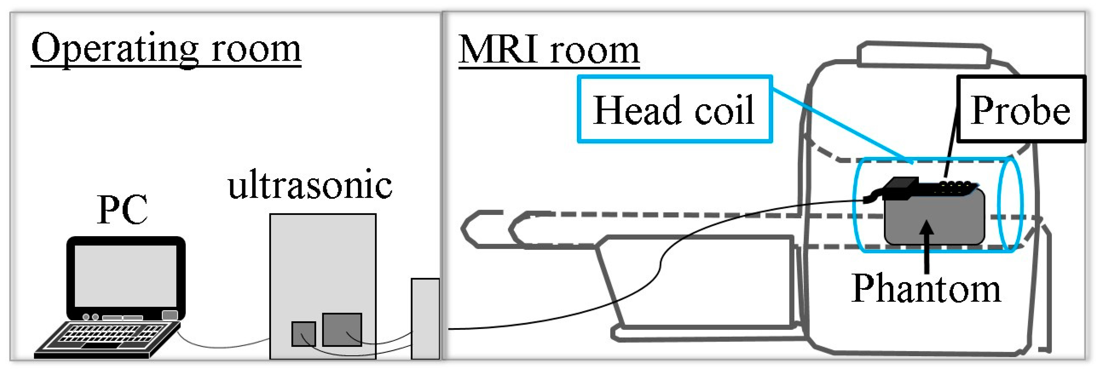
2.2. Simultaneous Multimodality Imaging System Using Ultrasound and Magnetic Resonance
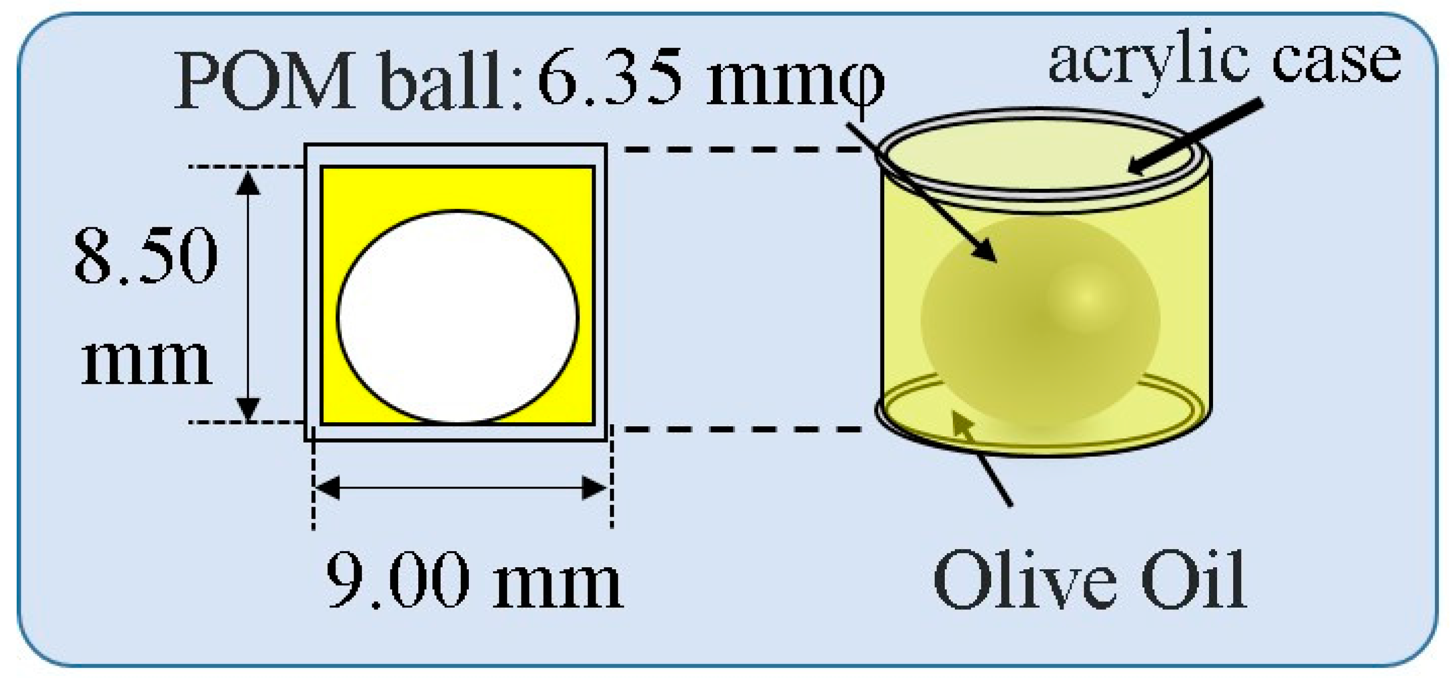
2.3. Measurement Method of Sound Velocity in Human Crus
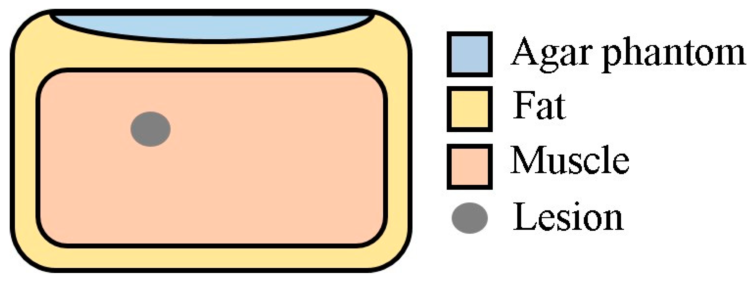
2.4. Experimental Imaging of an Abdominal Phantom using the Proposed Method of Compensating for the Sound Velocity Distribution to Correct Beamforming
2.5. Experimental Imaging of the Human Neck
3. Results and Discussion
3.1. Experimental Results of the Measurement of Sound Velocity in Human Crus
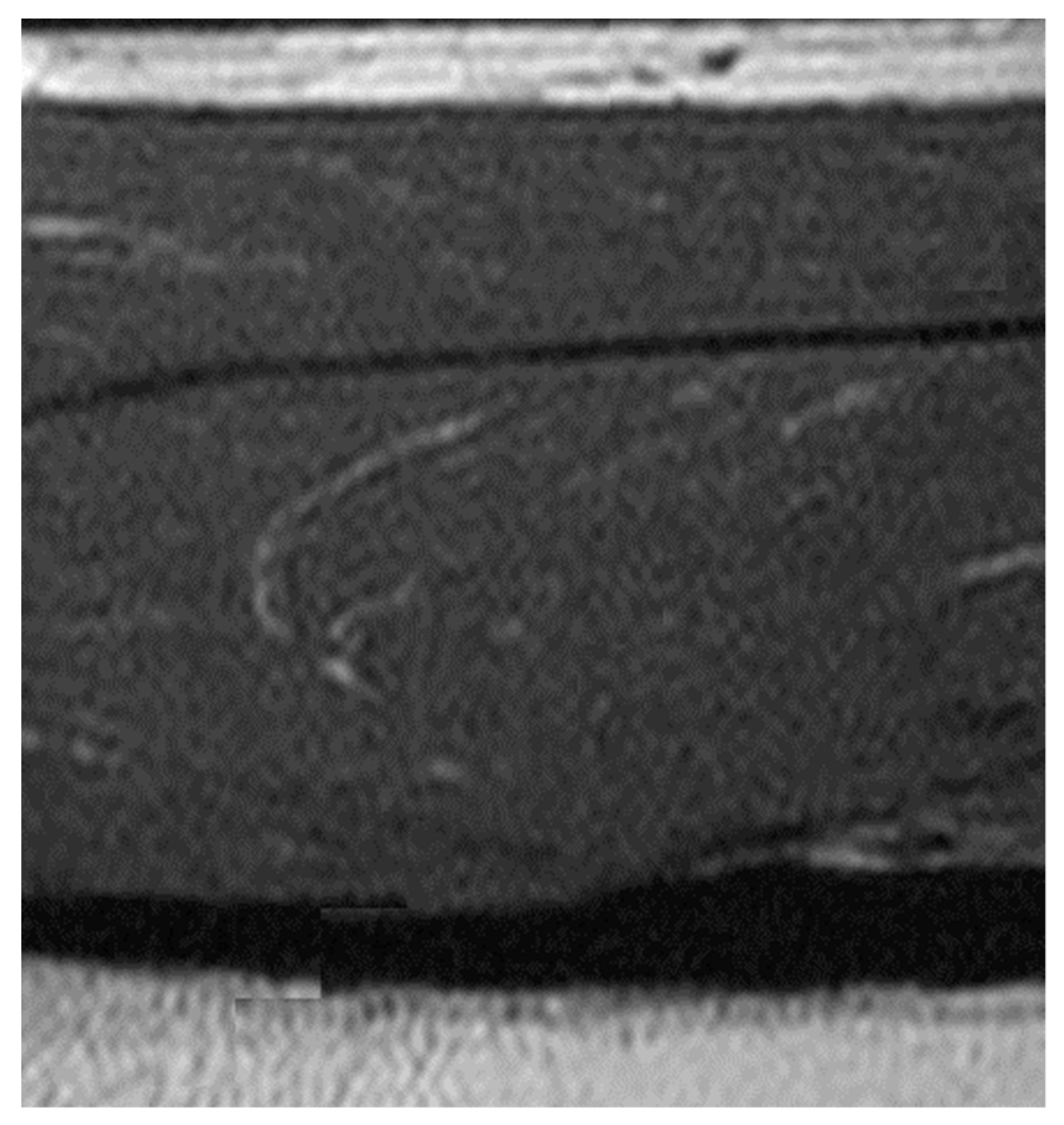
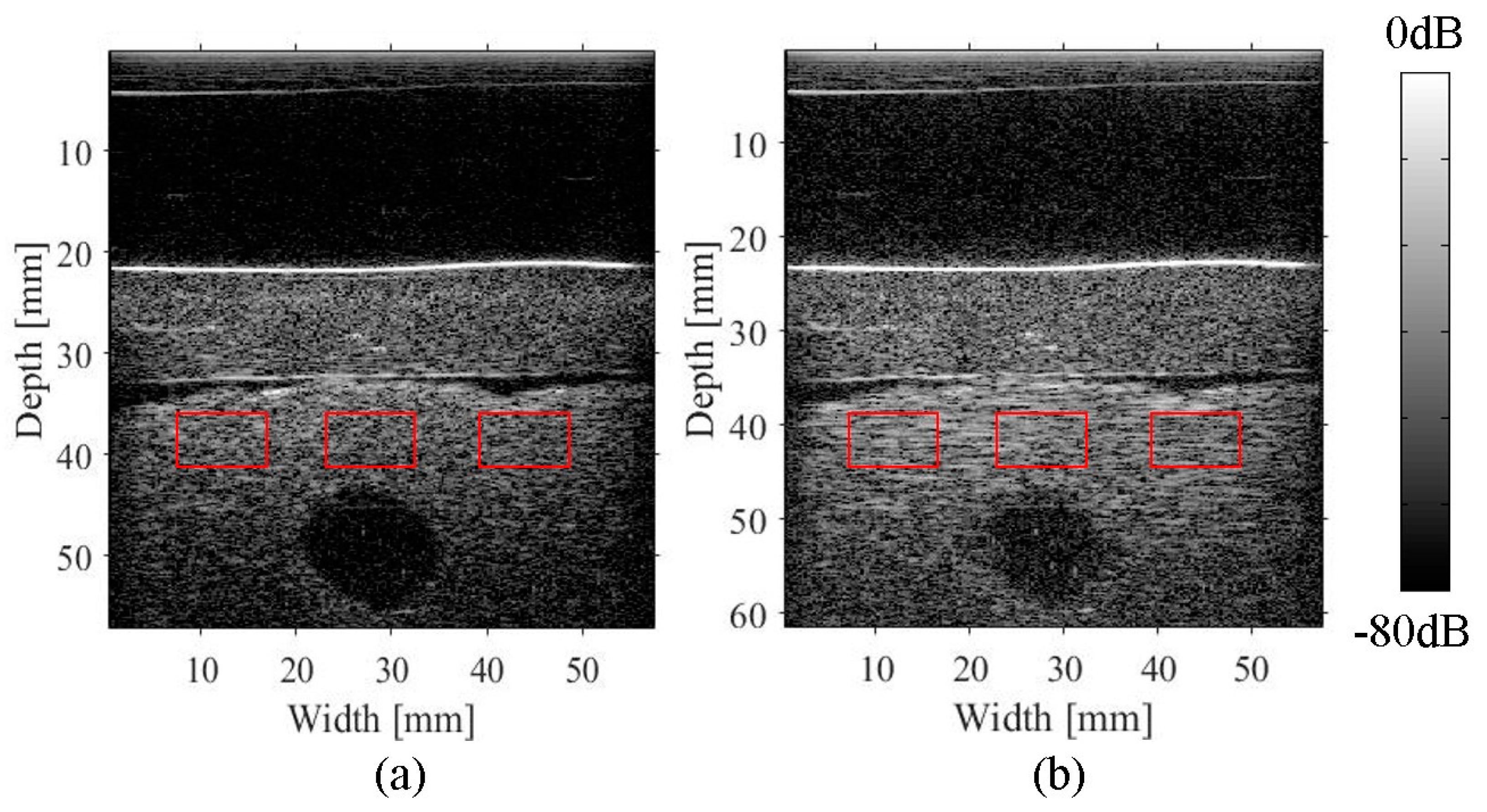
3.2. Imaging of an Abdominal Phantom
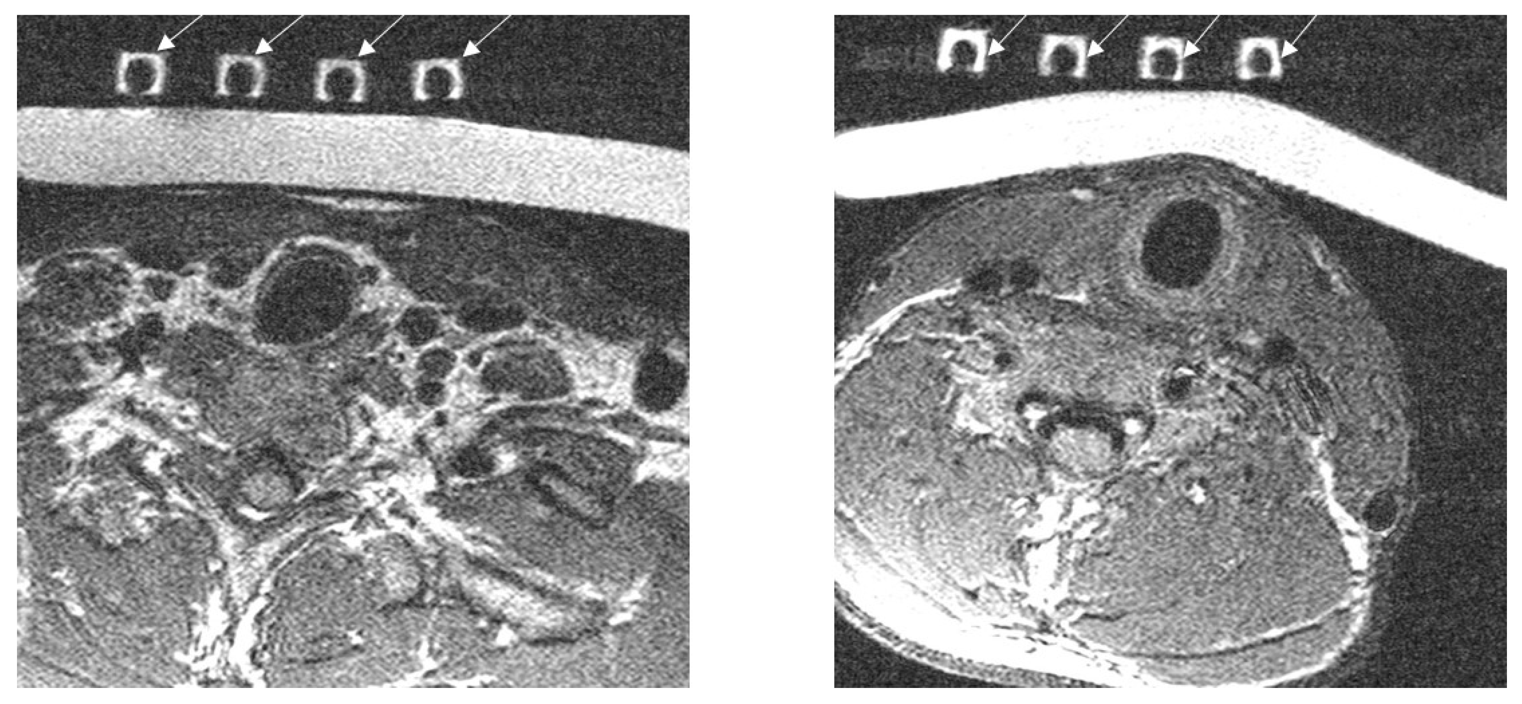
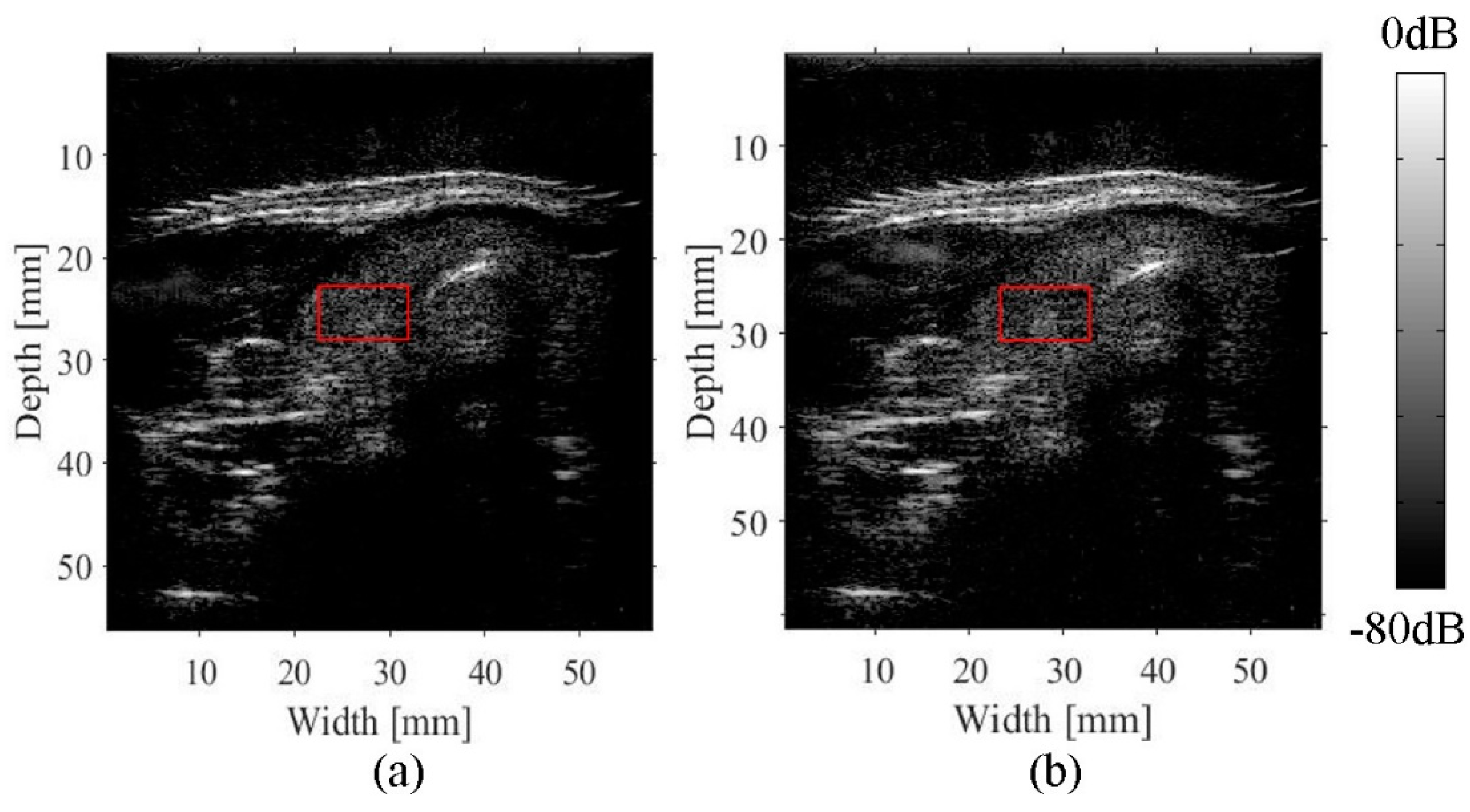
3.3. Imaging of the Neck
4. Conclusions
Author Contributions
Acknowledgments
Conflicts of Interest
References
- Goss, S.A.; Johnston, R.L.; Dunn, F. Comprehensive compilation of empirical ultrasonic properties of mammalian tissues. J. Acoust. Soc. Am. 1978, 64, 423–457. [Google Scholar] [CrossRef] [PubMed]
- Robinson, D.E.; Ophir, J.; Wilson, L.S.; Chen, C.F. Pulse-Echo Ultrasound Speed Measurements: Progress and Prospects. Ultrasound Med. Biol. 1991, 17, 633–646. [Google Scholar] [CrossRef]
- Kondo, M.; Takamizawa, K.; Hirama, M.; Okazaki, K.; Iinuma, K.; Takehara, Y. An evaluation of an in vivo local sound speed estimation technique by the crossed beam method. Ultrasound Med. Biol. 1990, 16, 65–72. [Google Scholar] [CrossRef]
- Anderson, M.E.; Trahey, G.E. The direct estimation of sound speed using pulse–echo ultrasound. J. Acoust. Soc. Am. 1998, 104, 3099–3106. [Google Scholar] [CrossRef] [PubMed]
- Benjamin, A.; Zubajlo, R.E.; Dhyani, M.; Samir, A.E.; Thomenius, K.E.; Grajo, J.R.; Anthony, B.W. Surgery for Obesity and Related Diseases: I. A Novel Approach to the Quantification of The Longitudinal Speed of Sound and Its Potenital for Tissue Characterization. Ultrasound Med. Biol. 2018. [Google Scholar] [CrossRef] [PubMed]
- Aoki, T.; Nitta, N.; Furukawa, A. Non-invasive speed of sound measurement in cartilage by use of combined magnetic resonance imaging and ultrasound: An initial study. Radiol. Phys. Technol. 2013, 6, 480–485. [Google Scholar] [CrossRef] [PubMed]
- Nitta, N.; Kaya, A.; Misawa, M.; Hyodo, K.; Numano, T. Accuracy improvement of multimodal measurement of speed of sound based on image processing. Jpn. J. Appl. Phys. 2017, 56, 07JF17. [Google Scholar] [CrossRef]
- Curiel, L.; Chopra, R.; Hynynen, K. Progress in Multimodality Imaging: Truly Simultaneous Ultrasound and Magnetic Resonance Imaging. IEEE Trans. Med. Imaging 2007, 26, 1740–1746. [Google Scholar] [CrossRef] [PubMed]
- Tang, A.M.; Kacher, D.F.; Lam, E.Y.; Wong, K.K.; Jolesz, F.A.; Yang, E.S. Simultaneous Ultrasound and MRI System for Breast Biopsy: Compatibility Assessment and Demonstration in a Dual Modality Phantom. IEEE Trans. Med. Imaging 2008, 27, 247–254. [Google Scholar] [CrossRef] [PubMed]
- Smith, W.A.; Shaulov, A.; Auld, B.A. Tailoring the properties of composite piezoelectric materials for medical ultrasonic transducers. In Proceedings of the 1985 IEEE Ultrasonics Symposium, San Francisco, CA, USA, 16–18 October 1985; pp. 642–647. [Google Scholar]
- Smith, W.A. Modeling 1–3 Composite Piezoelectrics: Hydrostatic Response. IEEE Trans. Ultrason. Ferroelectr. Freq. Control 1993, 40, 41–49. [Google Scholar] [CrossRef] [PubMed]
- Lynch, T.; (Computerized Imaging Reference Systems, Incorporated (CIRS)). Personal communication, 2018.


| Bandwidth (MHz) | Number of Elements | Element Pitch (mm) | Element Size (mm) | Focal Length of Acoustic Lens (mm) |
|---|---|---|---|---|
| 5–8 | 192 | 0.30 | 8.0 × 0.20 | 20 |
| Maximum Number of Probe Interface Channels | Number of TX/RX Channels | A/D Resolution (Bits) | Sampling Frequency (Hz) | Memory Capacitance Channel (MB) |
|---|---|---|---|---|
| 256 | 128 | 12 | 31.25 | 256 |
| Sequence | TR | TE | Thickness | Slices | Frequency Encoding | Phase Encoding |
|---|---|---|---|---|---|---|
| SE | 937 ms | 19.7 ms | 2.0 mm | 30 | 256 | 180 |
| Sequence | TR | TE | Thickness | Slices | Frequency Encoding | Phase Encoding |
|---|---|---|---|---|---|---|
| SE | 1436 ms | 20 ms | 1.5 mm | 45 | 256 | 180 |
| Subject 1 | Subject 2 | Subject 3 | Average | References [1] | ||
|---|---|---|---|---|---|---|
| Fat layer | Length (mm) | 3.58 ± 0.1 | 4.63 ± 0.1 | 4.24 ± 0.1 | - | - |
| Time of flight (μs) | 5.02 ± 0.03 | 6.34 ± 0.03 | 5.86 ± 0.03 | - | - | |
| Sound velocity (m/s) | 1430 ± 40 | 1460 ± 30 | 1450 ± 40 | 1445 ± 20 | 1459–1479 | |
| Muscle tissue | Length (mm) | 15.00 ± 0.1 | 14.13 ± 0.1 | 15.7 ± 0.1 | - | - |
| Time of flight (μs) | 9.75 ± 0.03 | 17.92 ± 0.03 | 20.0 ± 0.03 | - | - | |
| Sound Velocity (m/s) | 1540 ± 10 | 1580 ± 10 | 1570 ± 10 | 1562 ± 30 | 1540–1566 |
| ROIs | The Half-Width of the Autocorrelation Function for a Compensated Image | The Half-Width of the Autocorrelation Function for a Conventional Image | Ratio of the Half-Width Improvement |
|---|---|---|---|
| Left square | 1.35 mm | 2.55 mm | 0.53 |
| Center square | 0.85 mm | 2.60 mm | 0.30 |
| Right square | 1.33 mm | 3.02 mm | 0.44 |
| Average | 1.18 mm | 2.72 mm | 0.43 |
© 2018 by the authors. Licensee MDPI, Basel, Switzerland. This article is an open access article distributed under the terms and conditions of the Creative Commons Attribution (CC BY) license (http://creativecommons.org/licenses/by/4.0/).
Share and Cite
Inagaki, K.; Arai, S.; Namekawa, K.; Akiyama, I. Sound Velocity Estimation and Beamform Correction by Simultaneous Multimodality Imaging with Ultrasound and Magnetic Resonance. Appl. Sci. 2018, 8, 2133. https://doi.org/10.3390/app8112133
Inagaki K, Arai S, Namekawa K, Akiyama I. Sound Velocity Estimation and Beamform Correction by Simultaneous Multimodality Imaging with Ultrasound and Magnetic Resonance. Applied Sciences. 2018; 8(11):2133. https://doi.org/10.3390/app8112133
Chicago/Turabian StyleInagaki, Ken, Shimpei Arai, Kengo Namekawa, and Iwaki Akiyama. 2018. "Sound Velocity Estimation and Beamform Correction by Simultaneous Multimodality Imaging with Ultrasound and Magnetic Resonance" Applied Sciences 8, no. 11: 2133. https://doi.org/10.3390/app8112133
APA StyleInagaki, K., Arai, S., Namekawa, K., & Akiyama, I. (2018). Sound Velocity Estimation and Beamform Correction by Simultaneous Multimodality Imaging with Ultrasound and Magnetic Resonance. Applied Sciences, 8(11), 2133. https://doi.org/10.3390/app8112133