A New Metaheuristic Inspired by the Vapour-Liquid Equilibrium for Continuous Optimization

Abstract

In this article, a novel optimization metaheuristic based on the vapour-liquid equilibrium is described to solve highly nonlinear optimization problems in continuous domains. During the search for the optimum, the procedure truly simulates the vapour-liquid equilibrium state of multiple binary chemical systems. Each decision variable of the optimization problem behaves as the molar fraction of the lightest component of a binary chemical system. The equilibrium state of each system is modified several times, independently and gradually, in two opposite directions and at different rates. The best thermodynamic conditions of equilibrium for each system are searched and evaluated to identify the following step towards the solution of the optimization problem. While the search is carried out, the algorithm randomly accepts inadequate solutions. This process is done in a controlled way by setting a minimum acceptance probability to restart the exploration in other areas to prevent becoming trapped in local optimal solutions. Moreover, the range of each decision variable is reduced autonomously during the search. The algorithm reaches competitive results with those obtained by other stochastic algorithms when testing several benchmark functions, which allows us to conclude that our metaheuristic is a promising alternative in the optimization field.

1. Introduction

Over the past decades, conventional search methods have been applied to solve optimization problems, providing promising results in many cases. However, these methods may fail in more complex real-world problems where nonlinearity and multimodality are fundamental issues. If both constraints and objective functions are linear, the problem can be addressed with techniques specifically designed for solving linear programming problems, such as the simplex method. However, in most situations such problems are nonlinear, hindering the solution. Another difficulty arises when the problem is non-convex, the gradient is unknown, or the first derivatives do not exist. In these cases, it is not possible to apply gradient-based optimization methods, which is also common in real-world problems. Another challenge arises when the number of decision variables is large, affecting the search space. For instance, the well-known travelling salesman problem with a number of decision variables equalling 100 implies a number of possible combinations of $9.3\times {10}^{157}$, meaning that it is not practical to search all possible combinations. Thus, most real-world problems cannot be handled by conventional methods, which fall into local optima. Most real-world problems are NP-hard, which means that they require exponential time to be optimally solved. Thus, more efficient optimization methods are needed as metaheuristics [1].

Metaheuristics have shown promising results when solving extremely nonlinear and multimodal optimization problems. This type of algorithm combines randomization and local search to define strategies for solving difficult optimization problems with an approximate focus, i.e., it finds good solutions, but there is no guarantee that optimal solutions will be reached [1]. As expected, these techniques can be applied successfully to solve some problems, though they do not provide the desired success for others [2].

Different types of metaheuristics have been proposed in the literature during the last decades. Among the most promising metaheuristics are those inspired by natural phenomena (e.g., physical and chemical processes) and biological systems (fireflies, bees, and ant colonies) which have proven to be especially relevant for solving problems in different fields [3]. These metaheuristics can be classified depending on whether they are based on a single solution during the search (also called trajectory methods) or several solutions (also called population-based method) [4].

Among single solution-based metaheuristics, we focus on simulated annealing (SA) [5] (it is based on the annealing of metals, which consists of heating and then slowly cooling the metals to modify their physical properties), variable neighbourhood search (VNS) [6] (it performs the search by methodically modifying the local environment), greedy randomized adaptive search procedure (GRASP) [7] (an iterative procedure composed of an initial generation stage with heuristics and random selection processes and a second stage of improvement with local search), guided local search (GLS) [8] (it dynamically modifies the objective function during the search through a penalty factor, changing the search landscape to avoid being trapped in local optima), iterated local search (ILS) [9] (it performs a local search starting from an initial solution until a local minimum is reached, and then, the search starts again after modifying the solution found), and tabu search (TS) [10,11] (it considers an iterative local search procedure, which explores the search space from one solution to another, while accepting worsening movements if no improvement is available).

Population-based metaheuristics have been applied to different areas, including data mining [12], machine learning [13], computer science [14], simulation and system modelling [15], image processing [16], industry [17], and engineering and scheduling [18,19]. Some metaheuristic procedures supply better results in solving specific problems, whereas other metaheuristics are limited to certain domains of the decision variables; however, all of them are successful in solving optimization challenges [2]. Among these classic population-based methods, evolutionary algorithms (EAs) [7,20] constitute a set of algorithms based on Darwin’s evolutionary theory, where they start from an initial randomly generated population, which is improved over generations through recombination and mutation operators. Genetic algorithms (GAs) [21] are a subset of EAs, where the individuals in the population are in the form of an array or chromosome. Other important population-based metaheuristics are the gravitational search algorithm (GSA) [2] (it is based on the Newtonian law of gravity), the black hole (BH) algorithm [22] (where the best solution of a population is treated as a black hole that attracts other solutions or normal stars around it during the search), ant colony optimization (ACO) [23] (an ant colony searches for food according to the concentration of a chemical substance called a pheromone that ants deposit during the search), particle swarm optimization (PSO) [24] (it simulates bird behaviour using a simplified social model), the bat algorithm (BA) [25] (it is inspired by how bats look for their prey using echolocation), the artificial bee colony (ABC) algorithm [26] (it is inspired by the behaviour of honeybee swarms), and the artificial chemical reaction optimization algorithm (ACROA) [27] (it is inspired by some types and frequencies of certain chemical reactions). In the last five years, several optimization algorithms have been developed that consider novel search strategies and provide significant results. An important fraction of these methods is based on the social behaviour of a group of individuals of a determined live species. One of them considers, as a source of inspiration, human reasoning to make decisions when faced with fuzzy data [28]. Some of these techniques are: grey wolf optimizer (GWO) [29] (it imitates the command hierarchy and hunting strategy of grey wolves), the pity beetle algorithm (PBA) [30] (it was inspired by the grouping behaviour of the beetle Pityogenes chalcographus, looking for food and nests), shark smell optimization (SSO) [31] (it simulates the skill of a shark for finding their prey by using its sense of smell and moving toward the source of the odour), symbiotic organisms search (SOS) [32] (mimics the symbiotic interaction strategies followed by organisms to survive and propagate in the ecosystem), dolphin echolocation (DOE) [33] (it considers the echolocation system used by dolphins in searching for food), the whale optimization algorithm (WOA) [34] (it mimics the social behaviour of humpback whales), and the emperor penguin optimizer (EPO) [35] (it simulates the huddling behaviour of emperor penguins (Aptenodytes forsteri)).

This paper proposes a novel metaheuristic for continuous domains inspired by a physical-chemical process, i.e., the thermodynamic equilibrium between two fluid phases of a mixture composed by two chemical species: the vapour-liquid equilibrium (VLE) metaheuristic. The algorithm is based on the distribution of the most volatile component of a binary chemical mixture, between the liquid phase and the gas phase constituted by the vapour [36]. Thus, the search process of the metaheuristic is guided by the state changes of binary systems and uses the mathematical concept of the total differential. The behaviour of each binary system represents the movements or changes of a decision variable of an individual of a population. The metaheuristic also considers stochastic components to include diversity during the search process to avoid being trapped in local optima. Some examples of these components are found when generating new individuals, applying mutation operators, and enabling the exploration around worse solutions instead of better solutions. Some preliminary results obtained by the first version of VLE solving six benchmark functions were published previously [37]. Now, this paper describes the search mechanism of VLE in a deeper and more extensive way; it details the flowsheets of their main modules and presents new results obtained with more benchmark functions, which allows us to conclude that VLE is a promising alternative in the optimization field. This conclusion was the expected answer to our research question about whether changes in the thermodynamic state of a binary chemical system, in vapour-liquid equilibrium, would succeed or fail in developing a robust optimization technique to solve complex optimization problems if these changes were associated with each decision variable and were conducted towards the best equilibrium states, applying the concept of total differential.

The remainder of this work is structured as follows. Section 2 includes a conceptual explanation of VLE and a practical example of its application to a binary chemical system. Section 3 supplies a description of the optimization method by explaining how we perform the movements of the decision variables. Section 4 shows the mathematical models of the simulation used during the search for the optimal solution. Next, the movement operators, the parameters required, the method of characterizing the decision variables as chemical species, the inputs and outputs of the optimization procedure, the pseudocode of VLE and the flowsheets of the main modules of the algorithm are described in Section 5. For testing purposes, Section 6 describes the benchmark functions used as optimization problems and presents the optimization experimental results achieved. Finally, we present our conclusions and future work.

2. Vapour-Liquid Equilibrium for Binary Chemical Systems

In the chemical engineering field, the thermodynamic equilibrium ratio between two fluid phases is a common calculation. In this line, two classical calculation problems in the industry are multicomponent and flash distillation [38].

Let us assume a mixture of two fully miscible chemical species, such as a liquid and its vapour in thermodynamic equilibrium. Under saturated conditions, each of the two chemicals is present in all phases (vapour and liquid), and the chemical potential of each component between both phases is the same. In the case of an enclosed system, the total Gibbs free energy is at a minimum regarding all possible changes at a settled temperature and pressure [36,39]. This saturation condition is considered for designing the search process of the algorithm proposed in this paper. Specifically, we focus on bubble and dew points of a binary chemical mixture for designing the exploration phase of the algorithm and the flash distillation process for the exploitation phase.

To illustrate the concepts introduced before, we propose the following example. Let us assume a liquid mixture of 2-butanol and 1-butanol with a mole fraction of 0.352 and 0.648, respectively, as shown in Figure 1. For this binary system, the chemical species 2-butanol is more volatile than the chemical species 1-butanol. The mixture is enclosed in a cylinder with a piston at 98 ${}^{\circ }$C, and 525 mmHg, and the mixture is slowly heated at a constant pressure to a temperature of 104 ${}^{\circ }$C so that it is in equilibrium all the time.

Following the previous example, Figure 2 represents the phase diagram with the physical states of the system during the heating process, according to the system temperature (T), the molar fraction for vapour (v), and the liquid (l) phases of the most volatile chemical species in the mixture. The mixture (point A) is a subcooled liquid at 98 ${}^{\circ }$C. The system reaches the bubble point in point B at 99.9 ${}^{\circ }$C, which occurs when the first bubble of vapour appears. This vapour, represented by point $B^{{}^{\prime }}$ with mole fraction $v_{B^{{}^{\prime }}}$, is richer in 2-butanol than the original mixture, reducing the 2-butanol concentration in the remaining liquid phase. The horizontal line drawn by C-$C^{{}^{\prime }}$ represents a flash distillation, where the liquid and vapour are in equilibrium (Figure 3). As the temperature continues increasing, more vapour is formed from the liquid. Vapour and liquid are always in equilibrium; hence, the thermodynamic states of the two fluid phases lie along paths $B^{{}^{\prime }}D$ and $B{D}^{{}^{\prime }}$ and are linked everywhere by horizontal lines. The mixture reaches its dew point in point D at 102.6 ${}^{\circ }$C, which occurs when the last drop of liquid is left. From this moment, the system is a fully saturated vapour, reaching the last point E at 104.0 ${}^{\circ }$C. Note that, as the system is closed, the overall composition remains constant during the entire heating process. Thus, the state of the system is always represented by a point on the vertical line that goes from A to E.

3. Optimization Method Proposal

In this proposal, each decision variable is handled as the lightest chemical species of a given binary liquid mixture at a specified pressure and temperature, where the system pressure remains constant for all thermodynamic equilibrium calculations.

The optimization process starts from an initial randomly generated solution, which is iteratively modified through moving operators, generating new solutions. The algorithm includes an exploration mechanism to restart the iterative search, starting a new search process in a different area of the space of the solutions in the event that the previous search is considered exhausted. The maximum number of restarts is defined by a parameter of the metaheuristic, which controls the search orientation, making it more oriented to either exploration or exploitation. As expected, the maximum number of restarts will be fewer than the maximum number of movements allowed during the whole search process, which is also defined by another parameter of the metaheuristic. The search process ends when a stop criterion is reached, which can be the maximum number of movements or the maximum number of restarts.

Focusing on the exploration stage, the value of a decision variable is calculated according to the bubble and dew points of the binary chemical mixture associated with the same decision variable. This means that the value is adjusted according to the thermodynamic state that provides the best fitness value. Thus, the solution is evaluated for each value of the decision variable, while the other decision variables remain fixed in their final values after performing the previous movement. As a result, the fitness function is evaluated several times (indicated by a parameter) between two consecutive movements, by each decision variable.

Figure 4 shows a movement example performed during the exploration stage for an optimization problem in ${\mathbb{R}}^2$, for the decision variable $x_1$ between the iteration t and the iteration $t+1$. Figure 5 show movements for $x_2$. Specifically, these figures show phase diagrams (temperature versus mole fraction) for binary systems corresponding to acetone-acetonitrile (Figure 4) and benzene-toluene (Figure 5).

Focusing on the exploitation stage, the value of a decision variable is calculated based on the flash distillation process of the binary chemical mixture associated with the same decision variable. The value of the decision variable is adjusted based on the thermodynamic state providing the best fitness value in a similar way as for the exploration stage. Thus, Figure 6 shows how the new values of a decision variable are obtained during the exploitation stage, where $T_{fd}$ is the flash distillation temperature for the decision variable $x_1$. This figure corresponds to the same case of Figure 4.

The algorithm permits the stochastic modification of the chemical compounds and includes the random change of compositions of the binary liquid mixtures assigned to each decision variable. It also includes the acceptance of less than optimal solutions to avoid stagnation in local optimum. Finally, the technique includes the possibility to set up the search orientation of the algorithm.

4. Mathematical Models of Simulation Used During the Search for the Optimal Solution

In this section, we summarize the basic mathematical models for simulating the vapour-liquid equilibrium models, and the conditions that bubble point, dew point and flash distillation must satisfy.

4.1. Notation

The variables used to model the vapour-liquid equilibrium in a binary mixture of chemical species in its bubble point or dew point, or in a flash vapourization process of a binary mixture, are listed in

Table 1. Variables considered in the model.

Variable	Definition
F	Molar flow rate of the feed to the flash distillation vessel.
L, V	Liquid or vapour molar flow rates leaving the flash distillation vessel.
$f_j$	Overall molar composition of the compound j in the binary system or in the feed to the flash distillation vessel.
$l_j$, $v_j$	Molar fractions of the chemical species j in the liquid or vapour of the binary system, or in the liquid or vapour stream that leaves the flash distillation vessel.
$K_j$	Vapour-liquid saturation ratio or K-value of compound j.
$P_j^{*}$	Vapour pressure of chemical species j.
P	Total system pressure.
T	System temperature.
$A_j$, $B_j$, $C_j$	Constants A, B and C of Antoine’s equation [40] for vapour pressure calculation of the chemical species j.

. These definitions are required to write the fundamental equations that permit to obtain the mathematical expressions for the movement operators.

4.2. Mathematical Models

Equations to allow developing simple mathematical models for simulating the vapour-liquid equilibrium models.

Total Mass (Molar) Balance:

$$F=L+V$$

(1)

Mass (Molar) Balance for Component:

$$F{f}_j=L{l}_j+V{v}_{j}j\in \{1,2\}$$

(2)

$L/F$ Ratio:

$$\varphi =\frac{L}{F}$$

(3)

Unitary Mass (Molar) Balance:

$${\sum }_{j=1}^2{v}_j=1and{\sum }_{j=1}^2{l}_j=1$$

(4)

Phase Equilibrium Relationship:

$$v_j=K_j{l}_{j}j\in \{1,2\}or{l}_j=v_j/K_{j}j\in \{1,2\}$$

(5)

K-value (the vapour-liquid equilibrium is established by Raoult’s law [36]):

$$K_j=P_j^{*}/Pj\in \{1,2\}$$

(6)

Physical Properties: Vapour pressure of chemical species j at a given temperature T:

$$P_j^{*}=\exp [A_j-B_j/(T+C_j)]j\in \{1,2\}$$

(7)

Equation (8) must be satisfied at the bubble point to calculate its temperature $T_{BP}$ and the molar fraction of the first vapour produced, i.e., $v_j$. In these conditions, the vapour produced is in equilibrium with the liquid that has a composition $l_j$ = $f_j$. This equation is built by combining (4)–(7).

$${\sum }_{j=1}^2{v}_j=1=\sum _{j=1}^2\left(K_j{l}_j\right)$$

(8)

Similarly, the condition in (9) must be satisfied at the dew point to calculate its temperature $T_{DP}$ and the composition of the first drop of liquid produced, i.e., $l_j$. In these situations, the liquid produced is in equilibrium with the vapour phase, which has a molar composition $v_j$ = $f_j$. This equation is generated by combining (4)–(7).

$${\sum }_{j=1}^2{l}_j=1={\sum }_{j=1}^2(v_j/K_j)$$

(9)

Equations (8) and (9) are solved for temperature T, the bubble point or dew point, using the bisection numerical method [41].

Finally, for the flash distillation calculations, the condition in (10) must be satisfied in order to calculate the $\varphi$ = $L/F$ ratio and the molar fraction of the liquid formed, i.e., $l_j$. Under these conditions, the vapour phase formed is in equilibrium with the liquid phase which has a molar fraction $l_j$. Equation (10) is described by combining (1)–(7). It is solved for $\varphi$, also using the bisection numerical method [41].

$${\sum }_{j=1}^2{l}_j=1={\sum }_{j=1}^2\frac{f_j}{\varphi +(1-\varphi )K_j}$$

(10)

5. Algorithm

The algorithm considers a trustworthy strategy, novel movement operators, few tuning parameters, and the corresponding inputs and outputs.

5.1. Notation

The variables used in Equations (11) through (18) are listed in

Table 2. Variables considered in the algorithm.

Variable	Definition
$min$	Lower bound of $x_i$ in the real search space of $x_i$.
$max$	Upper bound of $x_i$ in the real search space of $x_i$; $max$ > $min$.
$nmin$	New lower bound for $x_i$, but in the molar fractions search space for $x_i$, i.e., zero, the minimum value of a molar fraction.
$nmax$	New upper bound for $x_i$, but in the molar fractions search space for $x_i$, i.e., one, the maximum value of a molar fraction.
$f_i$	Overall the mole fraction of the chemical species i, i.e., the species j = 1 (the most volatile compound) in the binary system of the decision variable i, or in the feed to the binary flash distillation vessel i.
$l_i$, $v_i$	Molar fractions of the chemical species i, i.e., the species j = 1 (the most volatile compound) in the liquid or vapour of the binary system of the decision variable i, or in the liquid or vapour stream that leaves the binary flash distillation vessel i.
$K_i$	Relationship of vapour-liquid equilibrium, or K-value, of the chemical species i, i.e., the species j = 1 (the most volatile compound) in the binary system for the decision variable i or in the binary flash distillation vessel i.
$\varphi$	$L/F$ ratio for the binary flash distillation vessel i.
G	Represents any of the constants A, B or C, of Antoine’s Equation.
$G_{il}$	Represents the lower bound of any of the constants A, B or C, of Antoine’s Equation.
$G_{sl}$	Represents the upper bound of any of the constants A, B or C, of Antoine’s Equation; $G_{sl}$ > $G_{il}$.
$x_i$	Decision variable i.
$x_i^{il}$	Lower bound of the decision variable $x_i$ in the real search space of $x_i$.
$x_i^{sl}$	Upper bound of the decision variable $x_i$ in the real search space of $x_i$; $x_i^{sl}$ > $x_i^{il}$.

.

5.2. Movement Operators

These operators correspond to the exploration and exploitation stages.

5.2.1. Search strategy

VLE begins the search by randomly creating a single starting solution. To do this, VLE considers, independently, the initial domain specified for each decision variable. Once this solution is created, VLE begins to explore its environment in a parallel search space, making a predefined number of changes in the value of each decision variable, keeping the other ones constant. This parameter is called alpha ($\alpha$) and it can be any odd number greater or equal to 3. If this number is equal to 5, the algorithm will apply, for each decision variable, $(5-1)/2=2$ times the bubble point operator and then $(5-1)/2=2$ times the dew point operator.

In other words, VLE starts creating new saturated binary mixes for each decision variable. For each created mixture, VLE evaluates its aptitude by using the equivalent values of each variable in its real domain. Next, for each decision variable, VLE looks for the most suitable mixture, that is, the one with the best aptitude, and thus the new value of the decision variable is determined. With the new values of the decision variables, the aptitude of the new solution is evaluated and compared with the best aptitude obtained from the last movement. If a better result is obtained, the procedure iterates until the change between the current aptitude and the best aptitude is less than an established tolerance or a stop criterion is reached. This criterion is usually the maximum number of movements or restarts. If the last solution found is the best one so far and it is no longer possible to continue exploring its environment, given the correspondence established between the real and parallel domains of the variables when the search starts or restarts, then VLE narrows the relationship between these two domains around the solution found. Once the relationship is narrowed, the exploitation phase begins. Nevertheless, if the result is worse, VLE either proceeds to accept the solution found or reject it to restart the search by creating a new initial solution elsewhere. The decision of acceptance or rejection depends on the probability of acceptance calculated for the solution found. If its probability of acceptance is grater than the predefined probability $beta$, then VLE accepts the solution, otherwise it is rejects it. The relationship between the real domain and the parallel domain is given by (12) or (14). Figure 7, Figure 8, Figure 9, Figure 10, Figure 11 and Figure 12, show the temperature diagrams versus molar fraction, in terms of ordered pairs, versus the respective values for each decision variable. The narrowing of this relationship is autonomous and depends exclusively on the equilibrium relationship between the chemical species that make up the binary mixture. If initially the relationship between these domains is from $[-100,+100]$ to $[0,1]$, and if the values of the decision variable closest to their current value are, for example, $+4$ and $+12.2$, assuming a value for the decision variable equal to $+7$, the narrowing for this variable will be from $[+4,+12.2]$ to $[0,1]$. In other words, VLE amplifies the environment closest to the solution, allowing the exploitation stage.

Summarizing, the exploration is performed covering a wide area that contains a certain number of binary chemical mixtures, all of them possible solutions of the optimization problem, and the exploitation is performed covering a reduced or local area that contains the same number of binary mixtures, with different compositions but very alike among them. Each of these areas defines a search table. A search table is a matrix used internally for each decision variable to perform a search around the current solution and select the more suitable movement for the corresponding decision variable, between iterations t and $t+1$. These areas are $wide$ $area$ $neighbourhoods$ (in the exploration stage), and $local$ $area$ $neighbourhoods$ (in the exploitation stage), respectively.

5.2.2. Exploration Stage

In the exploration stage, VLE considers two search operators: bubble point and dew point. These operators are given by (11) for the bubble point, and (13) for the dew point. Both operators “work” in the binary space ${\mathbb{R}}^2$, where $v_i$ and $l_i$ are real numbers that vary between 0 and 1.

In the case of the bubble point operator, from (5) we obtain (11), where $l_i\left(t\right)$ is equivalent to $x_i\left(t\right)$ (in the binary search space of the decision variable $x_i$) and $K_i\left(t\right)$ is the K-value for the compound i at temperature $T_{BP}$. The molar composition of the lightest compound of the liquid fraction, i.e., $l_i\left(t\right)$, is calculated by (12). This equation is a linear transformation of the values of a decision variable in the real domain $[min$, $max]$, into values of its equivalent variable in the real domain $[0,1]$.

$$l_i(t+1)=v_i\left(t\right)=K_i\left(t\right)l_i\left(t\right)i\in \{1,2,3,\dots ,n\}$$

(11)

The real domain $[0,1]$ is defined here as the search space for the decision variable $x_i$, whose true value belongs to the domain in $\mathbb{R}$ determined by the range $[min$, $max]$, for example $[-100$, $+100]$. In (12), $nmin=0$ and $nmax=1$ while $min=-100$ and $max=+100$. These two last bounds can be modified manually, while $nmin$ and $nmax$ are fixed because they are molar fractions, which have values between 0 and 1.

$$l_i\left(t\right)=\frac{nmax-nmin}{max-min}[x_i\left(t\right)-min]+nmini\in \{1,2,3,\dots ,n\}$$

(12)

For the dew point operator, from (5) we obtain (13), where $v_i\left(t\right)$ is equivalent to $x_i\left(t\right)$, but in the binary search space for $x_i$. The molar fraction of the lightest chemical compound in the vapour is given by (14).

$$l_i(t+1)=\frac{1}{K_i\left(t\right)}{v}_i\left(t\right)i\in \{1,2,3,\dots ,n\}$$

(13)

$$v_i\left(t\right)=\frac{nmax-nmin}{max-min}[x_i\left(t\right)-min]+nmini\in \{1,2,3,\dots ,n\}$$

(14)

If $\alpha$ is equal to 5, Equation (11) fills rows 4 and 5 of the search table of decision variable i, and Equation (13) rows 2 and 1 of same table. The corresponding value in the saturated search space for the current value in the real domain of the decision variable i, i.e., $x_i\left(t\right)$, is located in row 3 of the search table. The evaluation of the objective function is performed by varying the value of one decision variable by maintaining the values of all the other decision variables of the current solution to the problem.

The value of $x_i(t+1)$ is established by the molar fraction of the liquid phase that provides the best value of the optimization function among the five possible thermodynamic equilibrium states evaluated for $x_i$. This value is calculated by the inverse transformation (15), which takes the value of the molar fraction, and converts it into the respective value belonging to the correct search space.

$$x_i(t+1)=\frac{max-min}{nmax-nmin}[l_i(t+1)-nmin]+mini\in \{1,2,3,\dots ,n\}$$

(15)

For example, consider the search of the optimum of the sphere function using $\alpha =5$. If the current solution in ${\mathbb{R}}^3$ is $x_1\left(t\right)=-3.2$, $x_2\left(t\right)=-50.1$, and $x_3\left(t\right)=80.6$, the objective function value will be $9016.6$; the corresponding values of the molar fractions in ${\mathbb{R}}^2$ of each decision variable are $l_{1,3}=0.484$, $l_{1,3}=0.250$, and $l_{1,3}=0.903$, respectively. These values are put in the centre row of the corresponding search tables. For each decision variable, the algorithm will build the search tables using the bubble point and dew point operators, as Figure 7 shows for $x_2$. The molar fractions that correspond to these liquid mixtures for $x_2$ are converted to new possible real values in the iteration $t+1$. While the algorithm is generating the search table of $x_1$, the values of $x_2$ and $x_3$ remain unchanged, conserving the values of the iteration t, i.e., $-50.1$ and $80.6$, respectively. The same occurs for $x_2$ and $x_3$ when the search table for $x_2$ is built; in this case, the values of $x_1$ and $x_3$ remain constant for iteration t, and for $x_3$, it conserves the values of $x_1$ and $x_2$. For $x_2$, the algorithm evaluates the objective function considering all possible new equilibrium states, using the real values of each decision variable. Thus, each search table is completed.

Next, the algorithm explores each search table looking for the minimum value given by the objective function among the five possible thermodynamic states evaluated for each decision variable. As we can see in Figure 7, the best and new value for $x_2$ will be $x_2(t+1)=-8.5$. The same process is performed for $x_1$ and $x_3$, which results in a new value of $70.3$ for $x_3$ in the iteration $t+1$; at the same time, the value for $x_1$ does not change, i.e., it remains as $3.2$. This new value may appreciate in the central row of Figure 8. Therefore, the new values for the decision variables at iteration $t+1$ will be $x_1(t+1)=-3.2$, $x_2(t+1)=-8.5$, and $x_3(t+1)=70.3$. With these new values, the objective function value will be $5032.1$. In this case, the algorithm updates the search tables as Figure 8 shows for $x_2$. In other words, the algorithm centres the new values in row 3 of each table, by scrolling the records up or down, and completes each search table.

Before starting the search for the next values of the decision variables, i.e., a new feasible solution, the algorithm updates, records and counts. The procedure continues until no change in the values for the decision variables is possible using the exploration stage operators. Figure 9 shows the last iteration for $x_2$ during this stage before beginning the exploitation stage.

5.2.3. Exploitation Stage

In the intensification stage, the new values for the decision variables are obtained by (10), calculating the previous $T_{fd}$ and $\varphi$.

For the flash distillation operator, we obtain (16) from (10), where $f_i\left(t\right)$ corresponds to $x_i\left(t\right)$, but in the binary space for $x_i$.

$$l_i(t+1)=\frac{1}{\varphi +(1-\varphi )K_i\left(t\right)}{f}_i\left(t\right)i\in \{1,2,3,\dots ,n\}$$

(16)

Starting from the last values obtained for the decision variables during the exploration stage, the flash distillation operator is now applied variable by variable. Thus, the flash distillation temperature for each decision variable has been calculated previously. The flash distillation temperatures are calculated as the average of the values of the temperatures that provide the two lowest and nearest values of the objective function, as Figure 10 and Figure 11 show. For example, with regard to Figure 12 for $x_1$, the lowest and nearest values of the objective function are 94.8 and 949.9. To put the next value for $x_1$ in row 3 of the search table, i.e., $x_1(t+1)$, the entire row 3 is moved to row 2 by updating it, as we can see in Figure 10. Then, considering a binary liquid mixture with a molar fraction equal to the molar fraction of the vapour that is in equilibrium with the liquid mixture, the flash distillation temperature translated to row 2 will be $T_{fd}=(T_{BP,2}+T_{BP,4})/2$. With this temperature, (10) is solved for $\varphi$. Once $\varphi$ and $T_{fd}$ are calculated, $l_1(t+1)$ is obtained from (16). The value of $x_i(t+1)$ is calculated by (15), i.e., using the inverse transformation equation. The procedure is repeated several times until no further change is possible in the downhill direction of the objective function using the flash operator or until a certain number of worse solutions has been accepted. These solutions will be accepted while the probability calculated for them is greater than the acceptance probability specified for this type of solution.

5.3. Parameters

The parameters required by VLE are: $\alpha$, $\beta$, $\delta$, $char$, and $tsys$.

The parameter $\alpha$ sets the number of solutions that will be evaluated in the search area, either in a big area (a $wide$ $area$ $neighbourhood$) or a little area (a $local$ $area$ $neighbourhood$). This parameter can be any odd number greater or equal to 3. By increasing $\alpha$, the number of evaluations increases between one effective movement and another, therefore increasing the possibility of finding a local optimum.

The parameter $\beta$ determines the minimum acceptance probability of bad solutions during the search process. The $\beta$ value can be fixed or variable. If it is considered variable, its value will gradually decrease as a function of m, the identification number of the current movement, from 1 to some value close to 0. The implicit assumption in making $\beta$ variable is that, as m increases, the probability of accepting poor quality solutions decreases. In other words, when beta is nearby 1, there are not so much opportunities as for intensifying the search in a $local$ $area$ $neighbourhood$ starting from a bad solution, but when it is nearby 0, the opportunities are high.

The parameter $\delta$ puts a limit in the descending movements, allowing the algorithm to leave the local area when not any appreciable change is obtained in the fitness during the descend.

The parameter $char$ allows characterizes again the chemical species after each restart. This parameter can be equal 1 or 0. The chemical species are characterised again when $char$ is equal to 1. This parameter introduces high randomness in the search.

Last, the $tsys$ parameter establish the type of chemical system to be simmulated. The value is 1 for system with chemical compounds very similar between them, 2 for compounds not so similar or not so different between them, or 3 for very different chemical compounds. If compounds are very similar or very different, the values of the decision values change slightly or significantly, respectively. In other words, the choice of the system, allows to direct the search either towards exploitation ($tsys$ = 1), towards a balance between exploitation and exploration ($tsys$ = 2), or towards exploration ($tsys$ = 3).

Summarizing, $alfa$, $beta$ and $tsys$ influence a lot in the search of the best solution.

The experiments considered $alfa$ from 3 to 35, $beta$ variable, and $tsys$ equal to 1, assuming that all the reference functions were extremely complex.

5.4. Characterization of Chemical Species

The optimization procedure requires the characterization of the chemical compounds. This is done through the vapour pressure, given by Antoine’s equation [40]. In this version, the chemical compounds are characterized autonomously, and they may change randomly in each restart until the search ends. The values for $A_i$, $B_i$ and $C_i$ are randomly generated according to (17), where G is equal to constants A, B or C, and $G^{il}$ and $G^{sl}$ are the lower and upper limits of G, respectively. The limit values of the Antoine’s constants (where P is the system pressure in $kPa$ and T is the system temperature in ${}^{\circ }$C) are the following: $[A^{il}=15.7527,A^{sl}=18.5875]$, $[B^{il}=2132.50,B^{sl}=3816.44]$ and $[C^{il}=-63.633,C^{sl}=-31.62]$.

$$G_i=G^{il}+Random[0,1](G^{sl}-G^{il})i\in \{1,2,3,\dots ,n\}$$

(17)

5.5. Inputs and Outputs

The input information is restricted to the finalization conditions and search parameters, whereas the output includes the records of all the iterations performed.

With regard to the inputs, it is necessary to specify three totalizers: number of movements $\left(M\right)$, number of restarts $\left(R\right)$, and number of decision variables $\left(D\right)$ of the optimization problem. In addition, it is necessary to start with an initial solution. For each decision variable $x_i$, the initial value is stochastically obtained according to (18), where $x^{il}$ and $x^{sl}$ are the lower and upper bounds of $x_i$, respectively. These bounds are usually fixed at $-100$ and $+100$, respectively, although they can have other values.

$$x_i=x_i^{il}+Random[0,1](x_i^{sl}-x_i^{il})i\in \{1,2,3,\dots ,n\}$$

(18)

In this version, one initial solution is also randomly created in each restart. In addition, for both search stages and each restart, it is necessary to specify the autonomous adjustment parameter of the search space subset, and the acceptance probability of worse solutions. Finally, all the functions tested are included in the code of the algorithm. Any other function can be added easily.

With regard to the outputs, they are the minimum value reached, the location of the optimum found, the convergence graph, and the records of all the movements. In each iteration, the best solution reached and its fitness is always shown. When a worse solution is accepted, the value of the objective function is also shown.

5.6. Pseudocodes

Algorithm 1 details the search procedure of VLE metaheuristic.

Algorithm 1: Main procedure of the vapour-liquid equilibrium-based metaheuristic.

1: read input data: $o.f$, $[decision$ $variable$ $ranges]$, D, E, M, and R   2: for ($e=1$:E) do 3:  initialize lists, neighbourhood, accountants $(m=1$, $r=1)$, totalizer of variables $(tvar=0)$  and status of variables $\left(svar\right(d)=0)$   4:  generate an initial solution randomly   5:  evaluate the fitness of the current solution   6:  update the list of $accepted$ and $best$ movements with the current solution   7:  update the list of $rejected$ movements with   8:  update the best solution with the current solution   9:  characterise the chemical components   10:  create the $wide$ $area$ $neighbourhood$ of solutions for each decision variable   11:  while (1) do 12:   if or ($m>M$, $r>R$) then 13:    break   14:   end if  15:   if ($tvar<D$) then 16:    search the best change for each decision variable in its corresponding neighbourhood   17:   else 18:    create a $local$ $area$ $neighbourhood$ for each decision variable with closer neighbours   19:   end if  20:   evaluate the fitness of the current solution   21:   evaluate the fitness change as $fcha=fit-bfit$   22:   if ($fcha<0$) then 23:    if ($fcha<\delta$) then 24:     make a downhill movement (a new best solution), and update the records   25:    else 26:     make an uphill movement   27:    end if  28:   else 29:    make an uphill movement   30:   end if  31:   display e, m, r, $bfit$   32:  end while  33:  save e, x, $bfit$, $convergence$ $graphic$   34: end for  35: sort$bfit$   36: save$box$$plot$   37: save$statistics$

Algorithm 2 describes the search procedure of the best change for each decision variable. This is done by sorting the saved values of the objective function when creating or updating the search neighbourhood. The lower value points out the best location, i.e., $bsite\left(d\right)$, and therefore the new value for decision variable d. This value is compared with $csite\left(d\right)$, the current location for decision variable d. If it is the same location, then it remains until the intensification procedure starts.

Algorithm 2: Procedure of search of the best change for each decision variable.

1: for ($d=1$:D) do 2:   sort the saved values of the objective function when creating or updating the search neighbourhood for d.   3:   if ($bsite\left(d\right)==csite\left(d\right)$) then 4:    assign $svar\left(d\right)=1$   5:    evaluate $tvar=tvar+1$   6:   end if  7: end for

Algorithm 3 shows that a $local$ $area$ $neighbourhood$ is created for d with solutions closer to the best solution found after reducing the range of decision variable d.

Algorithm 3: Procedure to create the $local$ $area$ $neighbourhood$ for each decision variable.

1: for ($d=1$:D) do 2:  reduce the range of search for decision variable d   3:  generate a new random value for decision variable d using the new range for d   4:  assign $svar\left(d\right)=0$   5: end for  6: initialize$tvar=0$   7: create the $local$ $area$ $neighbourhood$ of search of all decision variables

Algorithm 4 describes the descent procedure, that only accept the movement and update the records.

Algorithm 4: Downhill procedure.

1: evaluate$m=m+1$   2: update the list of $accepted$ movements with the current solution   3: update the list of $best$ movements with the current solution   4: update the list of $rejected$ movements with zeros   5: update the best solution with the current solution   6: update the neighbourhood of search of each decision variable descend towards the new solution accepted

Algorithm 5 explains the uphill procedure. When a worse solution is found, the algorithm calculates its acceptance probability assigning a random number between 0 and 1. This probability was defined as $P\left(B\right|A)$, where A is the event $find$ a $worse$ $solution$, and B is the event $accept$ a $worse$ $solution$. This probability is compared with the $\beta$ parameter. If $P\left(B\right|A)$ is greater or equal than $\beta$, then the algorithm accepts the movement and updates the records, otherwise the algorithm rejects the movement and restarts the search with the original search ranges.

Algorithm 5: Uphill procedure.

1: evaluate$P\left(B\right|A)=rand$   2: if ($P\left(B\right|A)\ge \beta$) then 3:  evaluate $m=m+1$   4:  update the list of $accepted$ movements with the current solution   5:  update the list of $best$ movements with the best previous solution   6:  update the list of $rejected$ movements with zeros   7:  update the best solution with the the best previous solution   8:  update the neighbourhood of search of each decision variable ascend towards the new solution accepted   9: else 10  evaluate $m=m+1$   11:  evaluate $r=r+1$   12:  initialize $tvar=0$   13:  change the status of all decision variable to 0   14:  generate an initial solution randomly   15:  evaluate the fitness of the current solution   16:  evaluate the fitness change as $fcha=fit-bfit$   17:  update the list of $accepted$ movements with the current solution   18:  if ($fcha<\delta$) then 19:   update the list of $best$ movements with the current solution   20:   update the best solution with the current solution   21:  else 22:   update the list of $best$ movements with the best previous solution   23:   update the best solution with the the best previous solution   24:  end if  25:  update the list of $rejected$ movements   26:  if ($char==1$) then 27:   characterise the chemical components   28:  end if  29:  create the $wide$ $area$ $neighbourhood$ of solutions for each decision variable   30: end if

6. Experimental Results

Next, we analyse the minimum values and their corresponding location reported by the benchmark functions considered. Additionally, we present the results obtained with our metaheuristic along with the respective analysis.

6.1. Benchmark Functions

VLE was tested using 15 mathematical benchmark functions frequently used by many researchers, Equations (19)–(33) [20,24,30,34,42], and 6 composite benchmark functions selected from the Technical Report of the CEC 2017 Special Session [43], as described in Table 6. The first set of benchmark functions includes four unimodal functions, Equations (19)–(22), five multimodal functions, Equations (23)–(27), and six multimodal functions with fix dimensions, Equations (28)–(33). Functions $f_1$ to $f_9$, i.e., Equations (19)–(27), are high-dimensional problems. Functions $f_5$ to $f_9$, i.e., Equations (23)–(27), are a very difficult group of problems for optimization algorithms. In these problems, the number of local minima increases exponentially as the number of dimensions increases [20]. This set of multimodal functions is very important because it reflects the ability of startup from local optima and continues the search in another place in the search space. The number of dimensions is $n=30$ in Equations (19)–(27). The minimum values of all these functions and the corresponding solutions are given in

Table 3. Optimum values reported for the benchmark functions in the literature, with their corresponding solutions and search subsets.

BenFun	SeaSub	Opt	Sol
$f_1\left(X\right)$	${[-100,100]}^{30}$	0	${\left[0\right]}^{30}$
$f_2\left(X\right)$	${[-10,10]}^{30}$	0	${\left[0\right]}^{30}$
$f_3\left(X\right)$	${[-100,100]}^{30}$	0	${\left[0\right]}^{30}$
$f_4\left(X\right)$	${[-30,30]}^{30}$	0	${\left[1\right]}^{30}$
$f_5\left(X\right)$	${[-500,500]}^{30}$	−12,569.487	${\left[420.9687\right]}^{30}$
$f_6\left(X\right)$	${[-5.12,5.12]}^{30}$	0	${\left[0\right]}^{30}$
$f_7\left(X\right)$	${[-32,32]}^{30}$	0	${\left[0\right]}^{30}$
$f_8\left(X\right)$	${[-600,600]}^{30}$	0	${\left[0\right]}^{30}$
$f_9\left(X\right)$	${[-50,50]}^{30}$	0	${\left[1\right]}^{30}$
$f_{10}\left(X\right)$	${[-65.536,65.536]}^2$	1	${[-32]}^2$
$f_{11}\left(X\right)$	${[-5,5]}^2$	−1.0316285	$(0.08983,-0.7126)$ and ($-0.08983,0.7126$)
$f_{12}\left(X\right)$	$[-5,10]$ for $x_1$ and	0.397887	($-3.142,12.275$), (3.142, 2.275) and
	[0, 15] for $x_2$		(9.425, 2.425)
$f_{13}\left(X\right)$	${[-2,2]}^2$	3	($0,-1$)
$f_{14}\left(X\right)$	${[0,1]}^3$	−3.86	($0.114,0.556,0.852$)
$f_{15}\left(X\right)$	${[0,1]}^6$	−3.32	($0.201,0.150,0.477,0.275,0.311,0.657$)

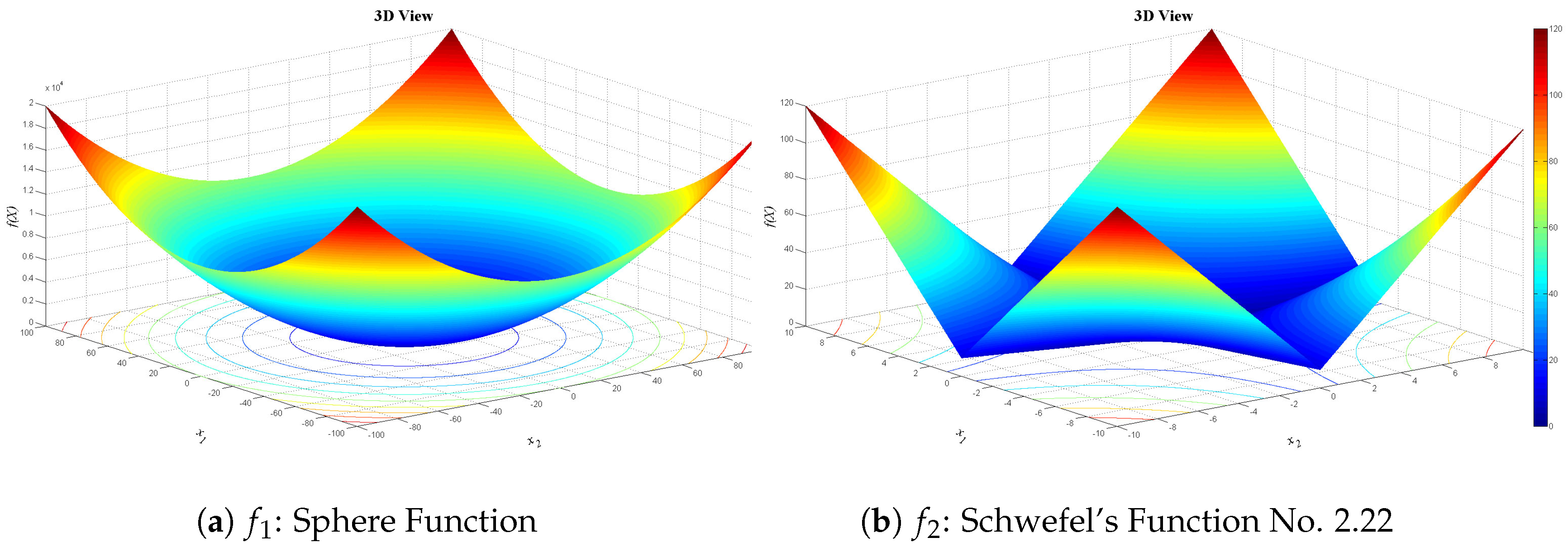
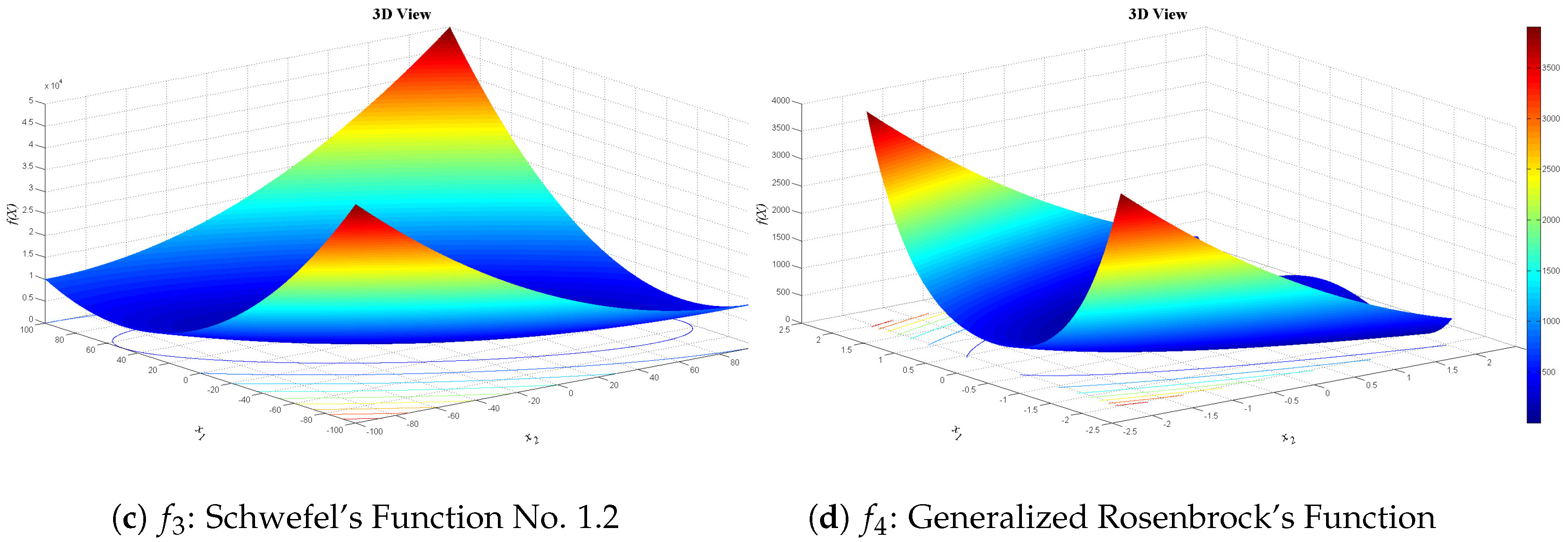
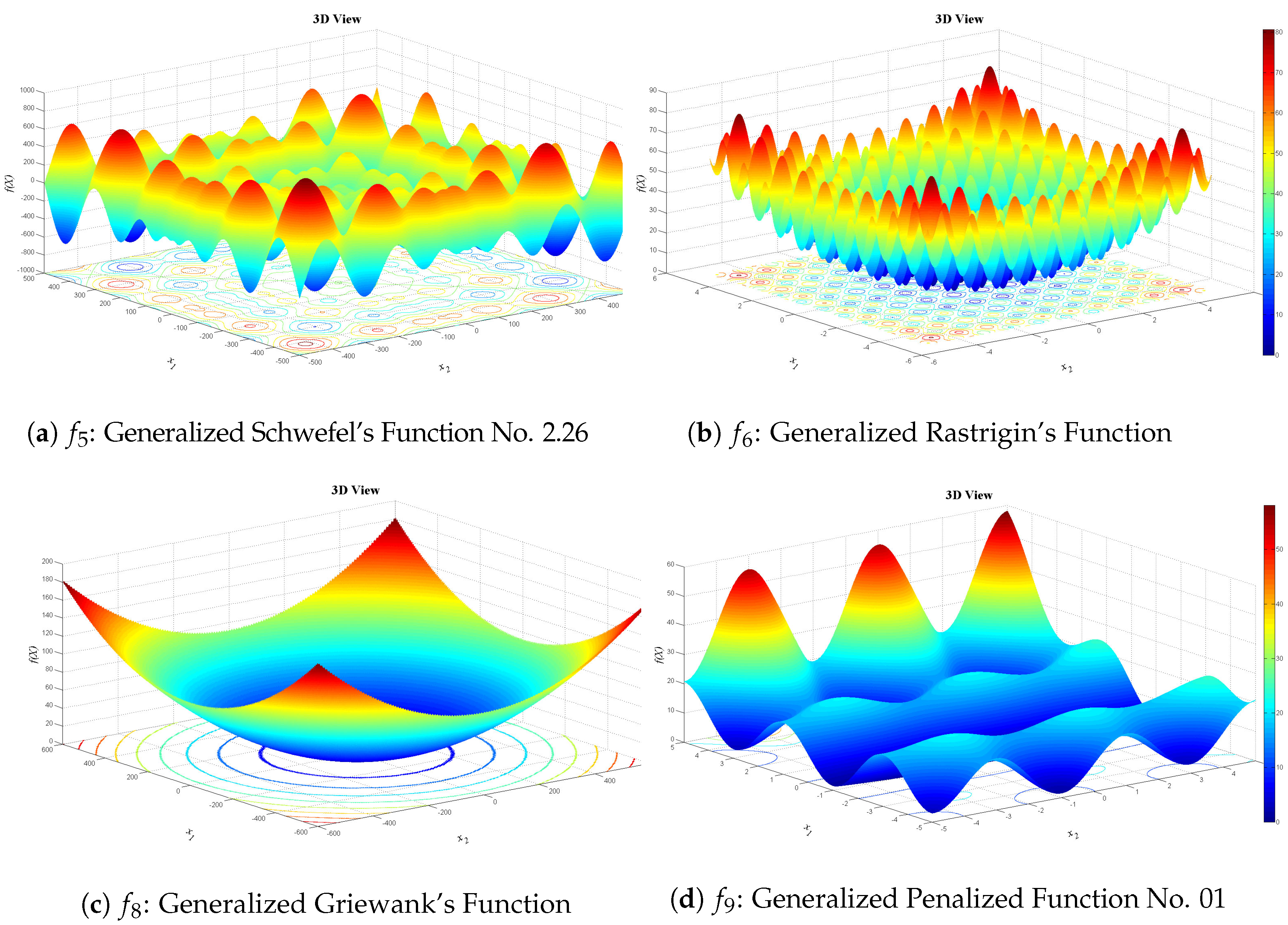
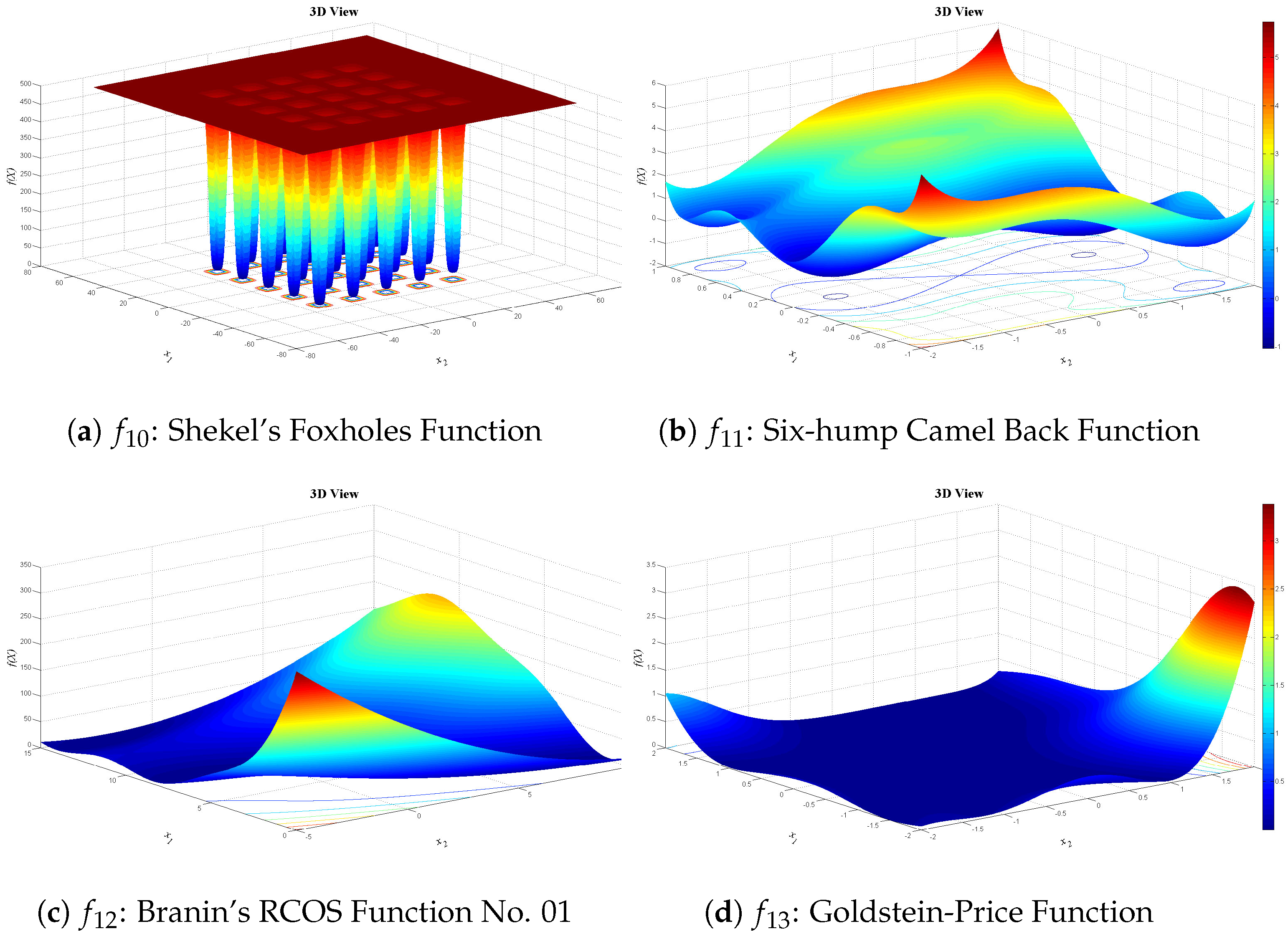
. Figure 13, Figure 14 and Figure 15 show 3D views of the first set of benchmark functions utilized in our experiments.

Unimodal test functions:

Sphere Function:

$$f_1\left(X\right)={\sum }_{i=1}^n{x}_i^2$$

(19)

Schwefel’s Function No. 2.22:

$$f_2\left(X\right)={\sum }_{i=1}^n|x_i|+{\prod }_{i=1}^n\left|x_i\right|$$

(20)

Schwefel’s Function No. 1.2:

$$f_3\left(X\right)={\sum }_{i=1}^n{\left({\sum }_{j=1}^i{x}_j\right)}^2$$

(21)

Generalized Rosenbrock’s Function:

$$f_4\left(X\right)={\sum }_{i=1}^{n-1}\left[100{(x_{i+1}-x_i^2)}^2+{(x_i-1)}^2\right]$$

(22)

Multimodal test functions:

Generalized Schwefel’s Function No. 2.26:

$$f_5\left(X\right)=-{\sum }_{i=1}^n\left(x_i\sin \left(\sqrt{|x_i|}\right)\right)$$

(23)

Generalized Rastrigin’s Function:

$$f_6\left(X\right)={\sum }_{i=1}^n\left[x_i^2-10\cos \left(2\pi x_i\right)+10\right]$$

(24)

Ackley’s Function:

$$\begin{array}{c}{f}_7\left(X\right)=-20\exp \left(-0.2\sqrt{\frac{1}{n}{\sum }_{i=1}^n{x}_i^2}\right)-\exp \left(\frac{1}{n}{\sum }_{i=1}^n\cos \left(2\pi x_i\right)\right)+20+e\end{array}$$

(25)

Generalized Griewank’s Function:

$$f_8\left(X\right)=\frac{1}{4000}{\sum }_{i=1}^n{x}_i^2-{\prod }_{i=1}^n\cos \left(\frac{x_i}{\sqrt{i}}\right)+1$$

(26)

Generalized Penalized Function:

$$\begin{array}{c}{f}_9\left(X\right)=\frac{\pi }{n}\left\{10{\sin }^2\left(\pi y_1\right)+\sum _{i=1}^{n-1}{\left(y_i-1\right)}^2\left[1+10{\sin }^2\left(\pi y_{i+1}\right)\right]+{\left(y_n-1\right)}^2\right\}\\ +\sum _{i=1}^{n}u\left(x_i,10,100,4\right)\end{array}$$

(27)

where $u(x_i,a,k,m)$ is equal to

$$\begin{array}{ccc}k{(x_i-a)}^m\hfill & \mathrm{if}& x_i>a,\hfill \\ 0\hfill & \mathrm{if}& -a\le x_i\le a,\mathrm{and}\hfill \\ k{(-x_i-a)}^m\hfill & \mathrm{if}& x_i<-a.\hfill \end{array}$$

and

$$\begin{array}{c}\hfill l{y}_i=1+\frac{1}{4}\left(x_i+1\right)\end{array}$$

Multimodal test functions with fixed dimensions:

Shekel’s Foxholes Function:

$$f_{10}\left(X\right)={\left[\frac{1}{500}+{\sum }_{j=1}^{25}\frac{1}{j+{\sum }_{i=1}^2{\left(x_i-a_{ij}\right)}^6}\right]}^{-1}$$

(28)

where

$$a_{ij}=\left[\begin{array}{cccccccccc}-32& -16& 0& 16& 32& -32& \dots & 0& 16& 32\\ -32& -32& -32& -32& -32& -16& \dots & 32& 32& 32\end{array}\right]$$

Six-hump Camel Back Function:

$$f_{11}\left(X\right)=4x_1^2-2.1x_1^4+\frac{1}{3}{x}_1^6+x_1{x}_2-4x_2^2+4x_2^4$$

(29)

Branin’s Function:

$$f_{12}\left(X\right)={\left(x_2-\frac{5.1}{4{\pi }^2}{x}_1^2+\frac{5}{\pi }{x}_1-6\right)}^2+10\left(1-\frac{1}{8\pi }\right)\cos x_1+10$$

(30)

Goldstein-Price Function:

$$\begin{array}{c}{f}_{13}\left(X\right)=\left[1+{\left(x_1+x_2+1\right)}^2\left(19-14x_1+3x_1^2-14x_2+6x_1{x}_2+3x_2^2\right)\right]\\ \left[30+{\left(2x_1-3x_2\right)}^2\left(18-32x_1+12x_1^2+48x_2-36x_1{x}_2+27x_2^2\right)\right]\end{array}$$

(31)

Hartman’s Family Function:

$$f_{14}\left(X\right)={-\sum }_{i=1}^4{c}_i\exp \left[{-\sum }_{j=1}^{n=3}{a}_{ij}{\left(x_j-p_{ij}\right)}^2\right]$$

(32)

$$f_{15}\left(X\right)={-\sum }_{i=1}^4{c}_i\exp \left[{-\sum }_{j=1}^{n=6}{a}_{ij}{\left(x_j-p_{ij}\right)}^2\right]$$

(33)

where $a_{ij}$, $c_i$ and $p_{ij}$, for $f_{14}\left(X\right)$, i.e., $n=3$, are given in

Table 4. Values of $a_{ij}$, $c_i$, and $p_{ij}$ for function $f_{14}\left(X\right)$; $n=3$ and $j=1,2,3$.

i	${\mathit{a}}_{\mathit{ij}}$			${\mathit{c}}_{\mathit{i}}$	${\mathit{p}}_{\mathit{ij}}$
1	3	10	30	1	0.3689	0.1170	0.2673
2	0.1	10	35	1.2	0.4699	0.4387	0.7470
3	3	10	30	3	0.1091	0.8732	0.5547
4	0.1	10	30	3.2	0.03815	0.5743	0.8828

, and for $f_{15}\left(X\right)$, i.e., $n=6$, in

Table 5. Values of $a_{ij}$, $c_i$, and $p_{ij}$ for function $f_{15}\left(X\right)$; $n=6$ and $j=1,2,\dots ,6$.

i	${\mathit{a}}_{\mathit{ij}}$						${\mathit{c}}_{\mathit{i}}$	${\mathit{p}}_{\mathit{ij}}$
1	10	3	17	3.5	1.7	8	1	0.131	0.169	0.556	0.012	0.828	0.588
2	0.05	10	17	0.1	8	14	1.2	0.232	0.413	0.830	0.373	0.100	0.999
3	3	3.5	1.7	10	17	8	3	0.234	0.141	0.352	0.288	0.304	0.665
4	17	8	0.05	10	0.1	14	3.2	0.404	0.882	0.873	0.574	0.109	0.038

.

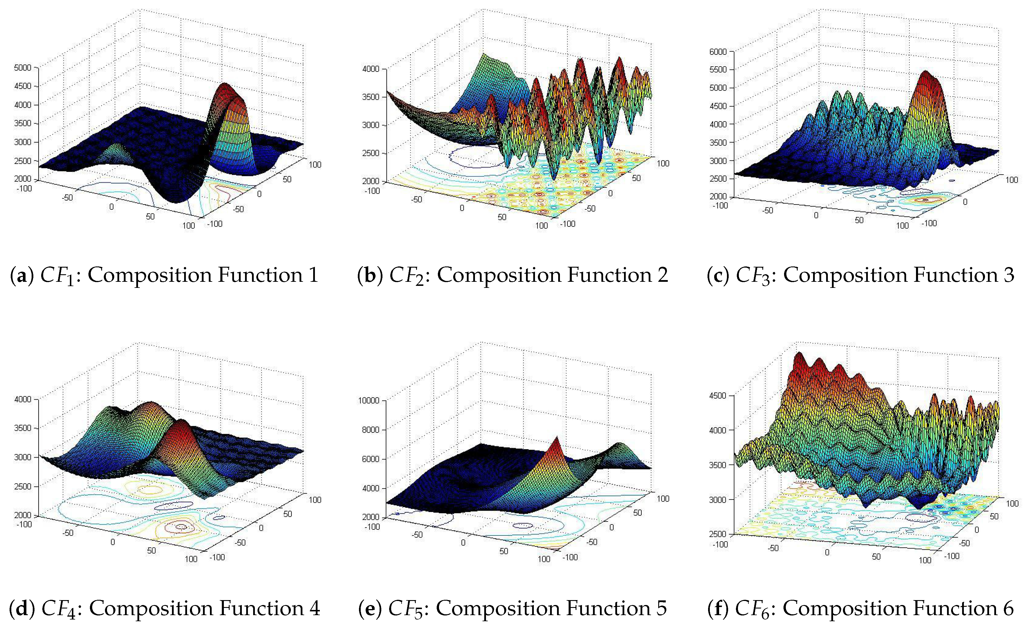
Regarding the second set of benchmark functions, all basic functions that have been used in the composition functions are shifted and rotated functions [43]. In addition, all composite functions are multimodal, non-separable, asymmetrical and have different properties around different local optima [43]. These properties create a high complexity in searching the optimum solution. Complete definitions of these functions are stated in the CEC 2017 Technical Report [43]. The number of dimensions and the search subset or range ($SeaSub$) were $n=10$ and $[-100$, $+100]$, respectively, for all composite functions utilized, as shown in

Table 6. Composite benchmark functions, CEC 2017 Test Suite [43]; $n=10$.

BenFun	Name	Search Subset	Optimal
$C{F}_1$	Composition Function 1 (Test Function No. 21)	${[-100,100]}^{10}$	2100
	N= 3
	$\sigma =[10,20,30]$, $\lambda =[1,1e-6,1]$
	$bias=[0,100,200]$
	$g_1$: Rosenbrock’s Function $F_4$’
	$g_2$: High Conditioned Elliptic Function $F_{11}$’
	$g_3$: Rastrigin’s Function $F_5$’
$C{F}_2$	Composition Function 2 (Test Function No. 22)	${[-100,100]}^{10}$	2200
	N = 3
	$\sigma =[10,20,30]$, $\lambda =[1,10,1]$
	$bias=[0,100,200]$
	$g_1$: Rastrigin’s Function $F_5$’
	$g_2$: Griewank’s Function $F_{15}$’
	$g_3$: Modified Schwefel’s Function $F_{10}$’
$C{F}_3$	Composition Function 3 (Test Function No. 23)	${[-100,100]}^{10}$	2300
	N = 4
	$\sigma =[10,20,30,40]$, $\lambda =[1,10,1,1]$
	$bias=[0,100,200,300]$
	$g_1$: Rosenbrock’s Function $F_4$’
	$g_2$: Ackley’s Function $F_{13}$’
	$g_3$: Modified Schwefel’s Function $F_{10}$’
	$g_4$: Rastrigin’s Function $F_5$’
$C{F}_4$	Composition Function 4 (Test Function No. 24)	${[-100,100]}^{10}$	2400
	N = 4
	$\sigma =[10,20,30,40]$, $\lambda =[10,1e-6,10,1]$
	$bias=[0,100,200,300]$
	$g_1$: Ackley’s Function $F_{13}$’
	$g_2$: High Conditioned Elliptic Function $F_{11}$’
	$g_3$: Girewank Function $F_{15}$’
	$g_4$: Rastrigin’s Function $F_5$’
$C{F}_5$	Composition Function 5 (Test Function No. 25)	${[-100,100]}^{10}$	2500
	N = 5
	$\sigma =[10,20,30,40,50]$, $\lambda =[10,1,10,1e-6,1]$
	$bias=[0,100,200,300,400]$
	$g_1$: Rastrigin’s Function $F_5$’
	$g_2$: Happycat Function $F_{17}$’
	$g_3$: Ackley Function $F_{13}$’
	$g_4$: Discus Function $F_{12}$’
	$g_5$: Rosenbrock’s Function $F_4$’
$C{F}_6$	Composition Function 6 (Test Function No. 26)	${[-100,100]}^{10}$	2600
	N = 5
	$\sigma =[10,20,20,30,40]$, $\lambda =[1e-26,10,1e-6,10,5e-4]$
	$bias=[0,100,200,300,400]$
	$g_1$: Expanded Scaffer’s $F_6$ Function $F_6$’
	$g_2$: Modified Schwefel’s Function $F_{10}$’
	$g_3$: Griewank’s Function $F_{15}$’
	$g_4$: Rosenbrock’s Function $F_4$’
	$g_5$: Rastrigin’s Function $F_5$’

. Figure 16 shows the 3D views of the benchmark composite functions chosen.

6.2. Results

Table 7. Optimization results of mathematical functions tested; $n=30$.

BenFun	Avg	StdDev	Med	Min	Opt	DMO	TPD	Max
$f_1$	4.4989 × 10${}^{-7}$	1.6413 × 10${}^{-6}$	4.4174 × 10${}^{-12}$	4.9649 × 10${}^{-21}$	0	4.9649 × 10${}^{-21}$	N/A	8.3455 × 10${}^{-6}$
$f_2$	3.0840 × 10${}^{-6}$	6.0498 × 10${}^{-6}$	2.4259 × 10${}^{-8}$	1.5549 × 10${}^{-13}$	0	1.5549 × 10${}^{-13}$	N/A	2.0115 × 10${}^{-5}$
$f_3$	5.2020	0.79863	5.3195	3.0218	0	3.0218	N/A	66.413
$f_4$	79.199	37.400	76.335	9.2776	0	9.2776	N/A	154.66
$f_5$	−1.2566 × 10${}^4$	68.705	−1.2566 × 10${}^4$	−1.2569 × 10${}^4$	−12,569.487	0.0000	0.0000%	−1.2190 × 10${}^4$
$f_6$	34.583	17.886	30.845	4.9748	0	4.9748	N/A	69.647
$f_7$	3.1704	3.9211	0.80444	9.6590 × 10${}^{-10}$	0	9.6590 × 10${}^{-10}$	N/A	13.777
$f_8$	0.50737	0.50405	0.36998	1.9418 × 10${}^{-7}$	0	1.9418 × 10${}^{-7}$	N/A	1.1885
$f_9$	0.23693	0.28773	0.11216	1.8385 × 10${}^{-16}$	0	1.8385 × 10${}^{-16}$	N/A	1.0792
$f_{10}$	0.99800	2.5294 × 10${}^{-7}$	0.99800	0.99800	1	−1.9962 × 10${}^{-3}$	−01.9962%	0.99801
$f_{11}$	−1.0315	1.8408 × 10${}^{-4}$	−1.0316	−1.0316	−1.0316285	0.0000	0.0000%	−1.0310
$f_{12}$	0.39815	4.5697 × 10${}^{-4}$	0.39794	0.39789	0.397887	1.0000 × 10${}^{-6}$	2.5133 × 10${}^{-4}$%	0.39951
$f_{13}$	3.0097	1.6256 × 10${}^{-2}$	3.0001	3.0000	3.00	0.0000	0.0000%	3.0510
$f_{14}$	−3.8628	6.6880 × 10${}^{-5}$	−3.8628	−3.8628	−3.86	−2.7821 × 10${}^{-3}$	7.2075 × 10${}^{-2}$%	−3.8624
$f_{15}$	−3.3179	2.1311 × 10${}^{-2}$	−3.3220	−3.3220	−3.32	−1.9952 × 10${}^{-3}$	6.0096 × 10${}^{-2}$%	−3.2031

and

Table 8. Search subsets considered and the optimum locations obtained.

BenFun	SeaSub	OptLoc
$f_1$	${[-100,100]}^{30}$	${\left[0\right]}^{30}$
$f_2$	${[-10,10]}^{30}$	${\left[0\right]}^{30}$
$f_3$	${[-1,1]}^{30}$	${\left[0\right]}^{30}$
$f_4$	${[-1,3]}^{30}$	${\left[1\right]}^{30}$
$f_5$	${[320,520]}^{30}$	${\left[420.9688\right]}^{30}$
$f_6$	${[-5.12,5.12]}^{30}$	${\left[0\right]}^{30}$
$f_7$	${[-32,32]}^{30}$	${\left[0\right]}^{30}$
$f_8$	${[-600,600]}^{30}$	${\left[0\right]}^{30}$
$f_9$	${[-50,50]}^{30}$	${[-1]}^{30}$
$f_{10}$	${[-65.536,65.536]}^2$	$(-31.98,-31.98)$
$f_{11}$	${[-5,5]}^2$	$(0.08984,-0.7127)$ and $(-0.08984,0.7127)$
$f_{12}$	$[-5,10]$ for $x_1$ and $[0,15]$ for $x_2$	$(-3.141,12.274)$, $(3.142,2.275)$ and $(9.425,2.475)$
$f_{13}$	${[-2,2]}^2$	$(0.000,-1.000)$
$f_{14}$	${[0,1]}^3$	$(0.115,0.556,0.853)$
$f_{15}$	${[0,1]}^6$	$(0.202,0.146,0.477,0.275,0.312,0.657)$

show the statistical results obtained with the first set of benchmark functions as follows: the benchmark function (BenFun), the average value obtained with the benchmark function (Avg), the standard deviation (StdDev), the median (Med), the minimum value achieved (Min), the optimal value (Opt), the true percentage deviation ($TPD$, %) or the difference between the minimum value achieved, and the optimal value published $\left(DMO\right)$, the worst result obtained or maximum value reached (Max), the search subset (SeaSub), and the optimal location (OptLoc). Optimal locations found were rounded to the values indicated under the OptLoc column in Table 8. For this set of functions, a total number of 1000 movements or 1000 restarts as the stop condition were considered for all the experiments, except in the experiments with functions f3, f4, f5 and f6; with those last functions, we use a maximum of 9000, 3000, 1500 and 4000, respectively. Very good results were obtained in 100.0% of the benchmark functions. Optimization results obtained by VLE were compared with the corresponding results reported for PSO [24], GSA [2], DE [42], and WOA [34], in [29,34]. All results obtained by VLE were rounded to four decimals. The results published for PSO, GSA, DE and WOA, were rounded in Table 7 and

Table 9. Averages and standard deviations obtained by VLE, and published for PSO, GSA, DE and WOA, using the classical benchmark functions; $n=30$.

BenFun	Statistic	VLE	PSO	GSA	DE	WOA
$f_1$	Avg	4.4989 × 10${}^{-7}$	1.3600 × 10${}^{-4}$	2.5300 × 10${}^{-16}$	8.2000 × 10${}^{-14}$	1.4100 × 10${}^{-30}$
	StdDev	1.413 × 10${}^{-6}$	2.0200 × 10${}^{-4}$	9.6700 × 10${}^{-17}$	5.9000 × 10${}^{-14}$	4.9100 × 10${}^{-30}$
$f_2$	Avg	3.0840 × 10${}^{-6}$	4.2144 × 10${}^{-2}$	5.5655 × 10${}^{-2}$	1.5000 × 10${}^{-9}$	1.0600 × 10${}^{-21}$
	StdDev	6.0498 × 10${}^{-6}$	4.5421 × 10${}^{-2}$	0.19407	9.9000 × 10${}^{-10}$	2.3900 × 10${}^{-21}$
$f_3$	Avg	5.2020	70.126	8.9653 × 10${}^2$	6.8000× 10${}^{-11}$	5.3900 × 10${}^{-7}$
	StdDev	0.79863	22.119	3.1896 × 10${}^2$	7.4000× 10${}^{-11}$	2.9300 × 10${}^{-6}$
$f_4$	Avg	79.199	96.718	67.543	0.0000	27.866
	StdDev	37.400	60.116	62.225	0.0000	0.76363
$f_5$	Avg	−1.2566 × 10${}^4$	−4.8413 × 10${}^3$	−2.8211 × 10${}^3$	−1.1080 × 10${}^4$	−5.0808 × 10${}^3$
	StdDev	68.705	1.1528 × 10${}^3$	4.9304 × 10${}^2$	5.7470 × 10${}^2$	6.9580 × 10${}^2$
$f_6$	Avg	34.5830	46.704	25.968	69.200	0.0000
	StdDev	17.8860	11.629	7.4701	38.800	0.0000
$f_7$	Avg	3.1704	0.27602	6.2087 × 10${}^{-2}$	9.7000× 10${}^{-8}$	7.4043
	StdDev	3.9211	0.50901	0.23628	4.2000 × 10${}^{-8}$	9.8976
$f_8$	Avg	0.50737	9.2150 × 10${}^{-3}$	27.702	0.0000	2.8900 × 10${}^{-4}$
	StdDev	0.50405	7.7240 × 10${}^{-3}$	5.0403	0.0000	1.5860 × 10${}^{-3}$
$f_9$	Avg	0.23693	6.9170 × 10${}^{-3}$	1.7996	7.9000 × 10${}^{-15}$	0.33968
	StdDev	0.28773	2.6301 × 10${}^{-2}$	0.95114	8.0000 × 10${}^{-15}$	0.214864
$f_{10}$	Avg	0.99800	3.6272	5.8598	0.99800	2.1120
	StdDev	2.5294 × 10${}^{-7}$	2.5608	3.8313	3.3000 × 10${}^{-16}$	2.4986
$f_{11}$	Avg	−1.0315	−1.0316	−1.0316	−1.0316	−1.0316
	StdDev	1.8408 × 10${}^{-4}$	6.2500 × 10${}^{-16}$	4.8800 × 10${}^{-16}$	3.1000 × 10${}^{-13}$	4.2000 × 10${}^{-7}$
$f_{12}$	Avg	0.39815	0.39789	0.39789	0.39789	0.39791
	StdDev	4.5697 × 10${}^{-4}$	0.0000	0.0000	9.9000 × 10${}^{-9}$	2.7000 × 10${}^{-5}$
$f_{13}$	Avg	3.0097	3.0000	3.0000	3.0000	3.0000
	StdDev	1.6256 × 10${}^{-2}$	1.3300 × 10${}^{-15}$	4.1700 × 10${}^{-15}$	2.0000 × 10${}^{-15}$	4.2200 × 10${}^{-15}$
$f_{14}$	Avg	−3.8628	−3.8628	−3.8628	N/A	−3.8562
	StdDev	6.6880 × 10${}^{-5}$	2.5800 × 10${}^{-15}$	2.2900 × 10${}^{-15}$	N/A	2.7060 × 10${}^{-3}$
$f_{15}$	Avg	−3.3179	−3.2663	−3.3178	N/A	−2.9811
	StdDev	2.1311 × 10${}^{-2}$	6.0516 × 10${}^{-2}$	2.3081 × 10${}^{-2}$	N/A	0.37665

to four decimals, using scientific notation, only for presentation purposes. However, all computations were realized using the reported decimals by their respective authors.

All experiments performed with VLE consisted of at least 31 executions with a certain set of VLE parameters. VLE parameters were tuned until a best possible solution was found. The technique for tuning was the parametric sweep. After this, the truncated mean was calculated by removing all possible strong outliers one by one. This process was done at 6.5% ($f_4$, $f_6$, and $f_7$), at 13.0% ($f_1$, $f_2$, $f_{10}$, $f_{11}$, and $f_{13}$) and at 20.0% ($f_8$, $f_9$, and $f_{12}$) depending on the number of strong outliers found. There were no outliers found with functions $f_3$, $f_5$, $f_{13}$, and $f_{14}$. All statistics reported for VLE in this work are presented according to this methodology. The reason for removing the strong outliers was to provide a measure of central tendency that was more representative of the distribution of the data obtained in each experiment.

A simple inspection of the values of the average fitness (Avg) of the objective function and of the corresponding standard deviation (StdDev), as it is shown in Table 9, permits us to establish a priori that VLE can compete successfully with a considerable part of this type of optimization problem, which is the scope of the present research. In other words, it can been seen that the results obtained by VLE are competitive.

We define the true percentage deviation ($TPD$) (34) as the measure of the search success. However, several of the benchmark functions tested have the optimal solutions as zero, and it is not possible to divide by zero. The ($TPD$) indicator was employed only for those functions whose optima ($Opt$) were different than zero. For the remaining functions, as the success indicator, we calculated the ($DMO$), the difference between the minimum achieved by VLE ($Min$) and the optimal value published ($Opt$) (35).

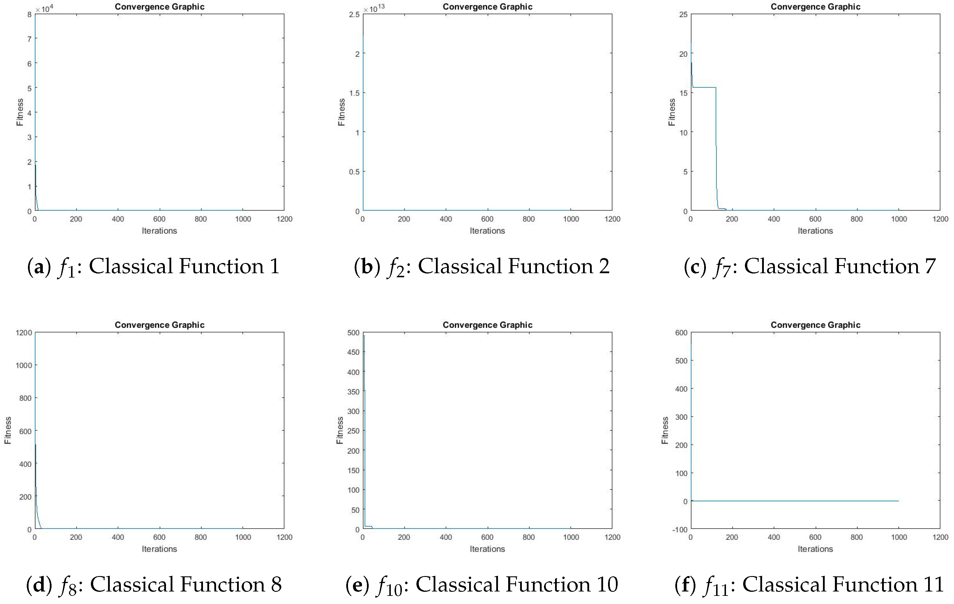
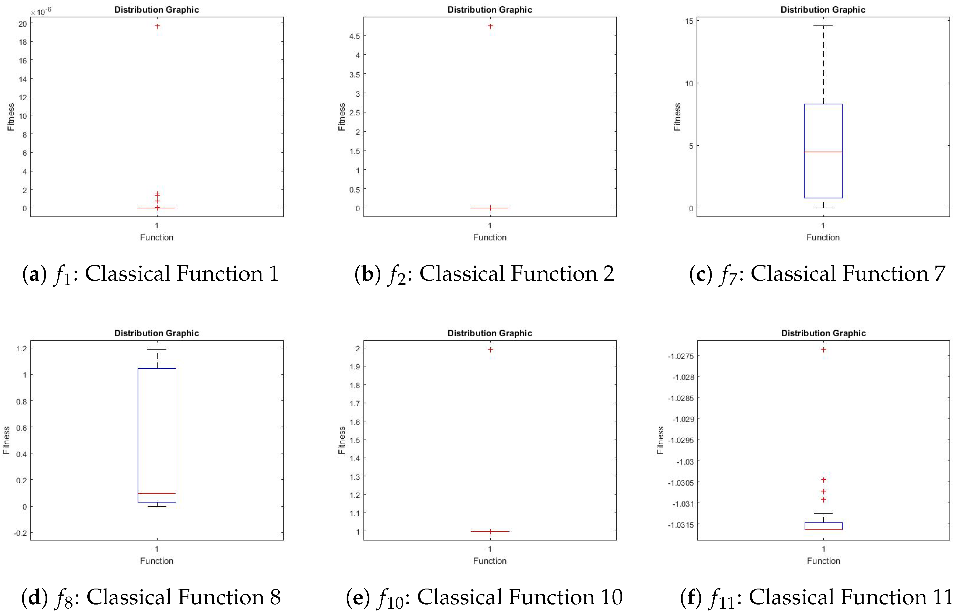
Figure 17 shows the convergence graphics obtained by VLE for benchmark functions $f_1$, $f_2$, $f_7$, $f_8$, $f_{10}$, and $f_{12}$. Figure 18 shows the distribution graphics obtained by VLE for these functions.

$$TPD=\left(\frac{Min-Opt}{Opt}\right)100$$

(34)

$$DMO=Min-Opt$$

(35)

The results were analysed from two points of view: (1) by making a thorough a comparative study of the mean values by function and metaheuristic; and (2) by using the root-mean-square error or RMSE. The comparative study allowed, in the first place, determining initially which VLE metaheuristic obtains a better result, and also determining the position of VLE on an evaluation scale of 1 to 5. In this evaluation scale, the number 1 is the best evaluation an algorithm can achieve. On the other hand, the use of the root-mean-square error, or RMSE, as a more robust statistic metric allowed the evaluation, in general terms, of which algorithm provided the averages that best fit the true optimum of the classical reference functions considered in this study.

Comparative study of the mean values:

Table 10. Averages comparison by function and metaheuristic (PSO, GSA, DE or WOA), using the classical benchmark functions; $n=30$.

BenFun	VLE-PSO	VLE	VLE-GSA	VLE	VLE-DE	VLE	VLE-WOA	VLE
$f_1$	−1.3555 × 10${}^{-4}$	1	4.4989 × 10${}^{-7}$		4.4989 × 10${}^{-7}$		4.4989 × 10${}^{-7}$
$f_2$	−4.2141 × 10${}^{-2}$	1	−5.5652 × 10${}^{-2}$	1	3.0825 × 10${}^{-6}$		3.0840 × 10${}^{-6}$
$f_3$	−649.24	1	−8.9133 × 10${}^2$	1	5.2020		5.2020
$f_4$	−175.19	1	11.656		79.199		51.333
$f_5$	−7.7247 × 10${}^3$	1	−9.7449 × 10${}^3$	1	−1.4859 × 10${}^3$	1	−7.4852 × 10${}^3$	1
$f_6$	−12.1210	1	8.6146		−34.6170	1	34.5830
$f_7$	2.8944		3.1083		3.1704		−4.2339	1
$f_8$	0.49816		−27.194	1	0.50737		0.50708
$f_9$	0.2301		−1.5627	1	0.2369		−0.1027	1
$f_{10}$	−2.6292	1	−4.8618	1	−4.0000 × 10${}^{-6}$	1	−1.1140	1
$f_{11}$	1.3000 × 10${}^{-4}$		1.3000 × 10${}^{-4}$		1.3000 × 10${}^{-4}$		1.3000 × 10${}^{-4}$
$f_{12}$	2.6300 × 10${}^{-4}$		2.6300 × 10${}^{-4}$		2.6300 × 10${}^{-4}$		2.3600 × 10${}^{-4}$
$f_{13}$	9.7000 × 10${}^{-3}$		9.7000 × 10${}^{-3}$		9.7000 × 10${}^{-3}$		9.7000 × 10${}^{-3}$
$f_{14}$	−2.0000 × 10${}^{-5}$	1	−2.0000 × 10${}^{-5}$	1	N/A		−6.6400 × 10${}^{-3}$	1
$f_{15}$	−5.1560 × 10${}^{-2}$	1	−1.2000 × 10${}^{-4}$	1	N/A		−0.33685	1
	VLE	9	VLE	8	VLE	3	VLE	6
	PSO	6	GSA	7	DE	10	WOA	9
	VLE	60.00%	VLE	53.33%	VLE	23.08%	VLE	40.00%

and

Table 11. Ranking of the optimization results (average fitness) obtained applying VLE, PSO,GSA,DE and WOA to the classical benchmark functions considered; $n=30$.

BenFun	1st	2nd	3rd	4th	5th	Rank	Subtotal
$f_1$	WOA	GSA	DE	VLE	PSO	4
$f_2$	WOA	DE	VLE	PSO	GSA	3
$f_3$	DE	WOA	VLE	PSO	GSA	3
$f_4$	DE	WOA	GSA	VLE	PSO	4	14
$f_5$	VLE	DE	WOA	PSO	GSA	1
$f_6$	WOA	GSA	VLE	PSO	DE	3
$f_7$	DE	GSA	PSO	VLE	WOA	4
$f_8$	DE	WOA	PSO	VLE	GSA	4
$f_9$	DE	PSO	VLE	WOA	GSA	3	15
$f_{10}$	VLE	DE	WOA	PSO	GSA	1
$f_{11}$	PSO,GSA,DE,WOA	VLE				2
$f_{12}$	PSO,GSA,DE	WOA	VLE			3
$f_{13}$	PSO,GSA,DE,WOA	VLE				2
$f_{14}$	VLE,PSO,GSA,WOA					1
$f_{15}$	VLE	GSA	PSO	WOA		1	10
							39
						$f_1$-$f_{15}$:	39/15 = 2.6
						$f_1$-$f_4$:	14/4 = 3.5
						$f_5$-$f_9$:	15/5 = 3.0
						$f_{10}$-$f_{15}$:	10/5 = 2.0

show the result of the comparative analysis of the performance of VLE compared to that of PSO, GSA, DE and WOA before the 15 reference functions already indicated. The results in Table 10 indicate that VLE shows a performance somewhat superior to that of PSO (60.00%), slightly higher than that of GSA (53.33%), and somewhat lower than that of WOA (40.00%). Since there is no information available for DE regarding functions $f_{14}$ and $f_{15}$, if these functions are excluded, it can be seen that VLE has low performance compared to DE (23.08%). Based on these observations, and the benchmark functions considered, it can be stated that, in general, and qualitative terms, VLE presents a competitive performance among PSO, GSA, DE, and WOA.I In quantitative terms, this analysis allows us to affirm that VLE has a weighted average performance of 44.83% among this group of functions and algorithms. In other words, considering this group of algorithms, this means that, if we take a population of 100 benchmark functions, VLE will deliver the best average fitness in 45 of these functions. The results of Table 11 show that, in general, the average performance of VLE is 2.6 on a scale of 1 to 5, with 1 being the best performance evaluation. This average global ranking considers that VLE reached first place 4 times, second place 2 times, third place 5 times, fourth place 4 times and that VLE never occupied fifth place. In addition to these results, it can be seen that the VLE ranking by type of benchmark function is 3.5 for the unimodal functions, 3.0 for the multimodal functions, and 2.0 for the multimodal test functions with a fixed number of dimensions. If functions $f_{14}$ and $f_{15}$ are excluded because there is no information available for DE, then the estimated global average performance of VLE is 2.85. In summary, if this indicator is rounded to the nearest integer, then VLE ranks third among the five metaheuristics considered and the 15 functions evaluated.

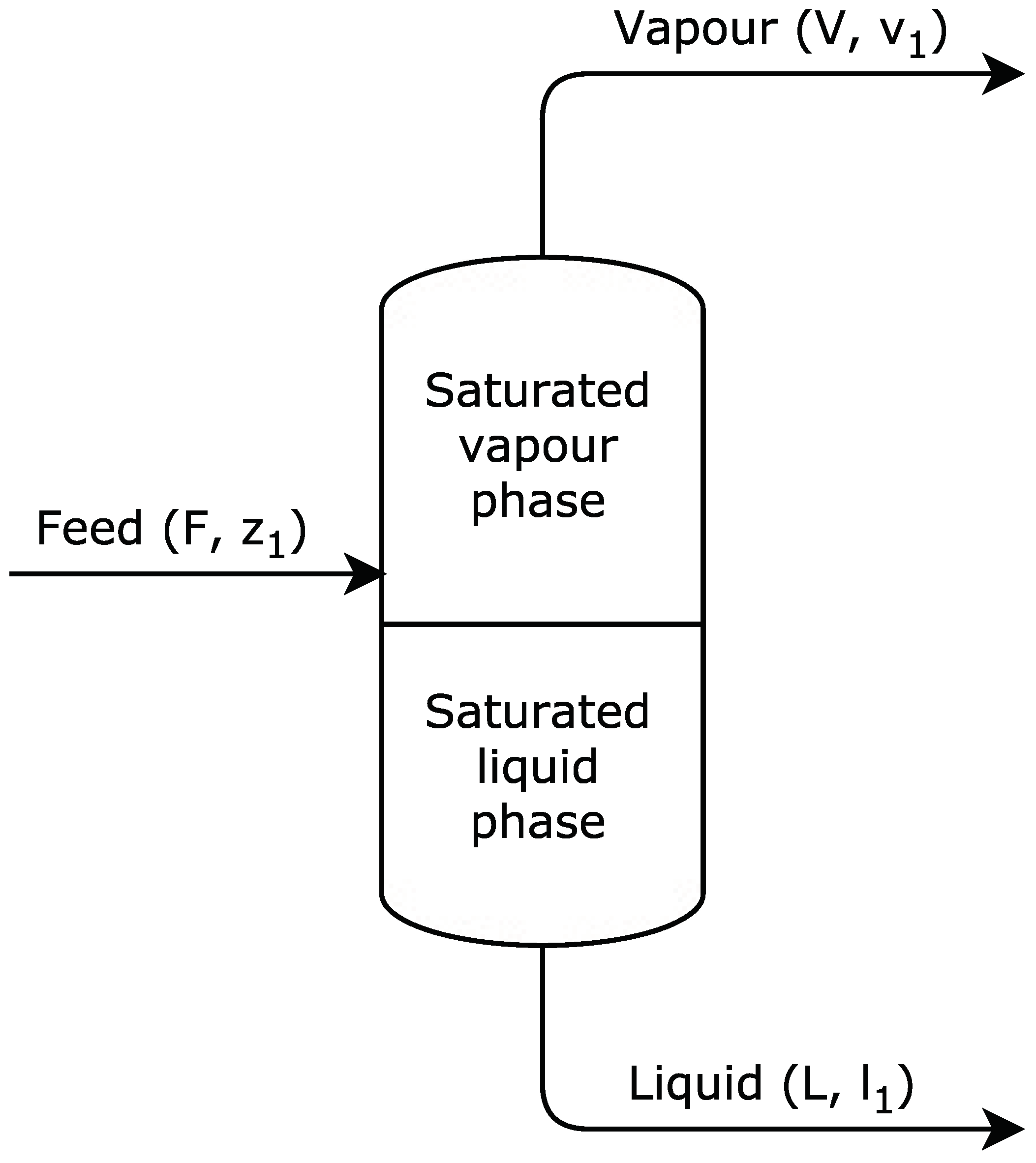
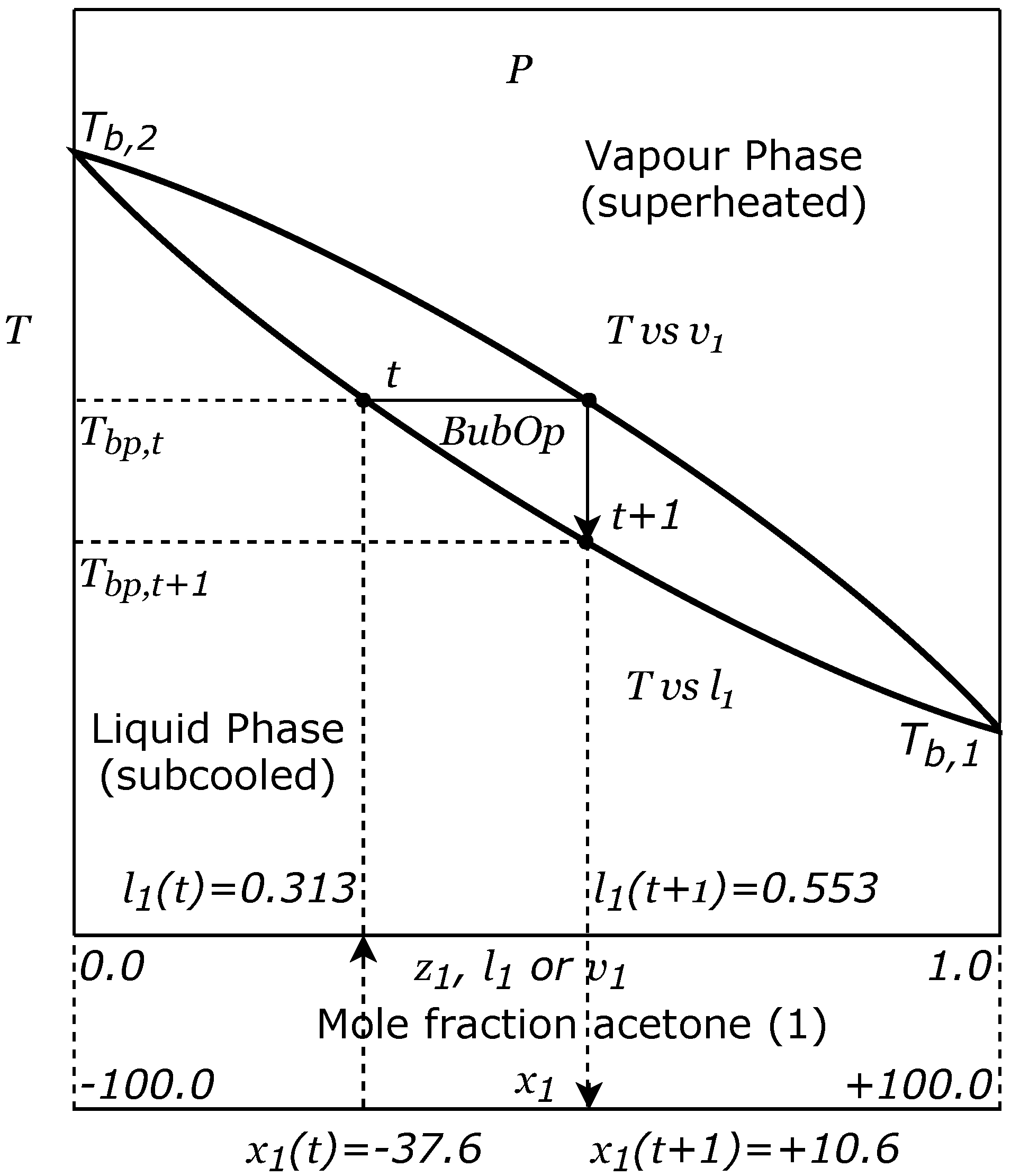
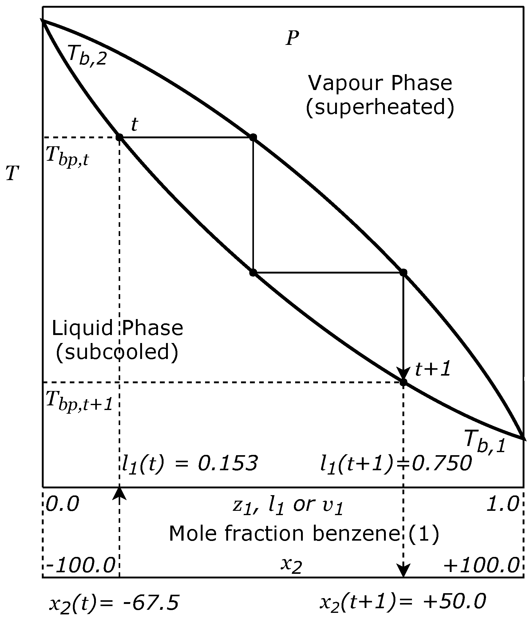
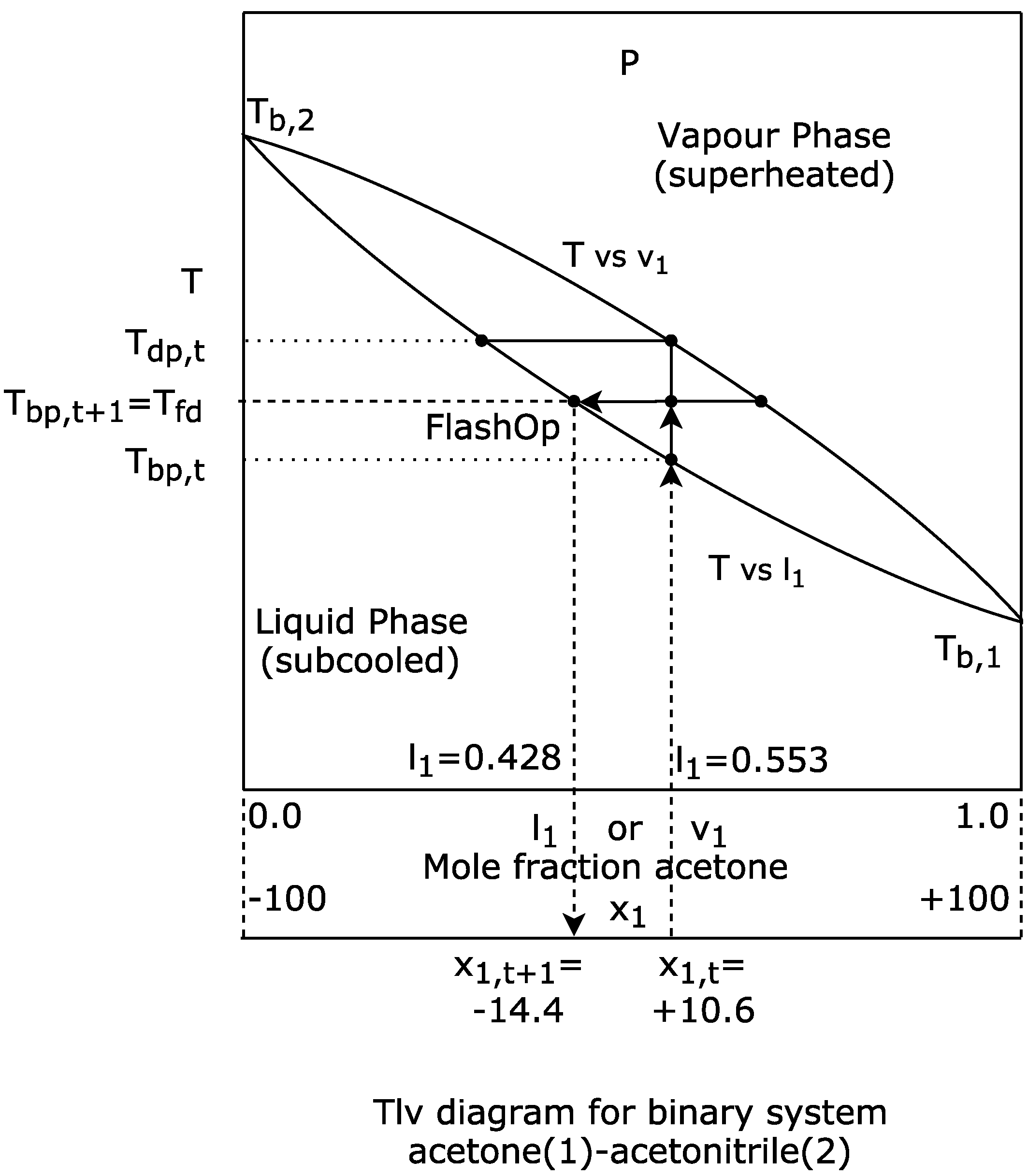
This comparative analysis allows us to corroborate that there is no metaheuristic that is capable of solving any optimization problem better than all the others. Some will work better than others for certain problems, while others will not perform as well [2]. In the case of VLE, this outcome may be due to the complexity of the algorithm, which simulates the physical-chemical process that served as inspiration. The real simulation restricts the potential capacity of the algorithm to reach more promising solutions with certain functions. For example, if a chemical species A and chemical species B are very similar to each other, the region enclosed between the saturation curves of the vapour-liquid equilibrium diagram will be very fine and will trend to be horizontal. This will produce more big steps around a good solution, than with a region of the same shape but with a greater incline, i.e., with a strong negative slope. In the limit, when chemical A is equal to chemical B, the system will be constituted by only one chemical species, i.e., will be a pure chemical species, so in this case, the binary diagram will be a horizontal straight line with no steps.

Root-mean-square error orRMSE:

Another general observation can be obtained if the root-mean-square error or $RMSE$ is used as shown in Equation (36). The $RMSE$ measures the average of the squared errors, that is, the difference between the estimator and what is estimated. In this case, the estimator considered is the average of the fitness of the reference function, determined by the optimization algorithm, and what is estimated is the value of the true optimum of the reference function. In Equation (36), $MH$ is any of the metaheuristics indicated, i.e., VLE, PSO, GSA, DE or WOA, and F is the number of data considered.

Table 12. Root-mean-square error ($RMSE$) of the results obtained among VLE and the reference metaheuristics; $n=30$.

BenFun	VLE	Opt	${(\mathit{VLE}-\mathit{Opt})}^2$	${(\mathit{PSO}-\mathit{Opt})}^2$	${(\mathit{SGA}-\mathit{Opt})}^2$	${(\mathit{DE}-\mathit{Opt})}^2$	${(\mathit{WOA}-\mathit{Opt})}^2$
$f_1$	4.4989 × 10${}^{-7}$	0.0000	2.0240 × 10${}^{-13}$	1.8496 × 10${}^{-8}$	6.4009 × 10${}^{-32}$	6.7240 × 10${}^{-27}$	1.9881 × 10${}^{-60}$
$f_2$	3.0840 × 10${}^{-6}$	0.0000	9.5111 × 10${}^{-12}$	1.7761 × 10${}^{-3}$	3.0975 × 10${}^{-3}$	2.2500 × 10${}^{-18}$	1.1236 × 10${}^{-42}$
$f_3$	5.2020	0.0000	27.061	4.9176 × 10${}^3$	8.0377 × 10${}^5$	4.6240 × 10${}^{-21}$	2.9052 × 10${}^{-13}$
$f_4$	79.199	0.0000	6.2725 × 10${}^3$	9.3544 × 10${}^3$	4.5621 × 10${}^3$	0.0000	7.7649 × 10${}^2$
$f_5$	−1.2566 × 10${}^4$	−1.2569 × 10${}^4$	1.2159 × 10	5.9725 × 10${}^7$	9.5032 × 10${}^7$	2.2183 × 10${}^6$	5.6081 × 10${}^7$
$f_6$	34.583	0.0000	1.1960 × 10${}^3$	2.1813 × 10${}^3$	6.7436 × 10${}^2$	4.7886 × 10${}^3$	0.0000
$f_7$	3.1704	0.0000	10.051	7.6184 × 10${}^{-2}$	3.8548 × 10${}^{-3}$	9.4090 × 10${}^{-15}$	54.824
$f_8$	0.50737	0.0000	0.25742	8.4916 × 10${}^{-5}$	7.6738 × 10${}^2$	0.0000	8.3521 × 10${}^{-8}$
$f_9$	0.23693	0.0000	5.6136 × 10${}^{-2}$	4.7845 × 10${}^{-5}$	3.2386	6.2410 × 10${}^{-29}$	0.11538
$f_{10}$	0.99800	1.0000	4.0000 × 10${}^{-6}$	6.9020	23.618	3.9840 × 10${}^{-6}$	1.2365
$f_{11}$	−1.0315	−1.0316	1.6512 × 10${}^{-8}$	2.2500 × 10${}^{-12}$	2.2500 × 10${}^{-12}$	2.2500 × 10${}^{-12}$	2.2500 × 10${}^{-12}$
$f_{12}$	0.39815	0.39789	6.9169 × 10${}^{-8}$	0.0000	0.0000	0.0000	7.2900× 10${}^{-10}$
$f_{13}$	3.0097	3.0000	9.4090 × 10${}^{-5}$	0.0000	0.0000	0.0000	0.0000
$f_{14}$	−3.8628	−3.8600	7.8400 × 10${}^{-6}$	7.7284 × 10${}^{-6}$	7.7284 × 10${}^{-6}$	N/A	1.4746 × 10${}^{-5}$
$f_{15}$	−3.3179	−3.3200	4.4100 × 10${}^{-6}$	2.8794 × 10${}^{-3}$	4.9284 × 10${}^{-6}$	N/A	0.11489
	$RMSE$	$f_1$-$f_{15}$	22.388	1.9957 × 10${}^3$	2.5277 × 10${}^3$	N/A	1.9336 × 10${}^3$
		$f_1$-$f_{13}$	24.048	2.1437 × 10${}^3$	2.7152 × 10${}^3$	4.1353 × 10${}^2$	2.0770 × 10${}^3$

shows the $RMSE$ values calculated for the 15 classical functions and the five algorithms considered in this study. Table 12 also presents the $RMSE$ values calculated for VLE and DE, excluding functions $f_{14}$ and $f_{15}$ due to lack of information for DE. With these results, it can be stated that, in general, the average fitness obtained by VLE is better adjusted to the true optimum of the reference functions than any of the published data sets for PSO, GSA, DE, and WOA. Considering the 15 classical functions, the $RMSE$ value for VLE is 22.388, for PSO it is 1995.7, for GSA it is 2527.7, and for WOA 1933.6. Excluding functions f14 and f15, the $RMSE$ values for VLE, PSO, GSA, DE and WOA are 24.048, 2143.7, 2715.2, 413.53 and 2077.0, respectively. According to this statistic metric, the $RMSE$ obtained by VLE under these circumstances is lower than that obtained by the other algorithms.

$$RMSE=\sqrt{\frac{{(Av{g}_{MH}-Opt)}^2}{F}}$$

(36)

Similarly,

Table 13. Optimization result of the composite functions tested, CEC 2017 Test Suite [43]; $n=10$.

BenFun	Avg	StdDev	Med	Min	Opt	DMO	TPD	Max
$C{F}_1$	2.2960 × 10${}^3$	54.296	2.3043 × 10${}^3$	2.1036 × 10${}^3$	2.1000 × 10${}^3$	3.6348	0.1371%	2.3606 × 10${}^3$
$C{F}_2$	2.2587 × 10${}^3$	28.176	2.2541 × 10${}^3$	2.2179 × 10${}^3$	2.2000 × 10${}^3$	17.9931	0.8179%	2.3111 × 10${}^3$
$C{F}_3$	2.6257 × 10${}^3$	86.929	2.6499 × 10${}^3$	2.3188 × 10${}^3$	2.3000 × 10${}^3$	18.8320	0.8188%	2.7007 × 10${}^3$
$C{F}_4$	2.5852 × 10${}^3$	79.818	2.6111 × 10${}^3$	2.4261 × 10${}^3$	2.4000 × 10${}^3$	26.1434	1.0893%	2.7536 × 10${}^3$
$C{F}_5$	2.9144 × 10${}^3$	99.702	2.9458 × 10${}^3$	2.6002 × 10${}^3$	2.5000 × 10${}^3$	100.2627	4.0100%	3.0067 × 10${}^3$
$C{F}_6$	2.9674 × 10${}^3$	1.8951 × 10${}^2$	3.0366 × 10${}^3$	2.6000 × 10${}^3$	2.6000 × 10${}^3$	0.0000	0.0000%	3.2266 × 10${}^3$

shows the statistical results obtained with the second set of optimization problems, i.e., the composite functions, which are the following: the benchmark function (BenFun), the average value (Avg), the standard deviation (StdDev), the median (Med), the minimum value achieved (Min), the optimal value published (Opt), the difference between the minimum value achieved (Min) and the optimal value published ($DMO$), the true percentage deviation ($TPD$, %), and the maximum value reached (Max). 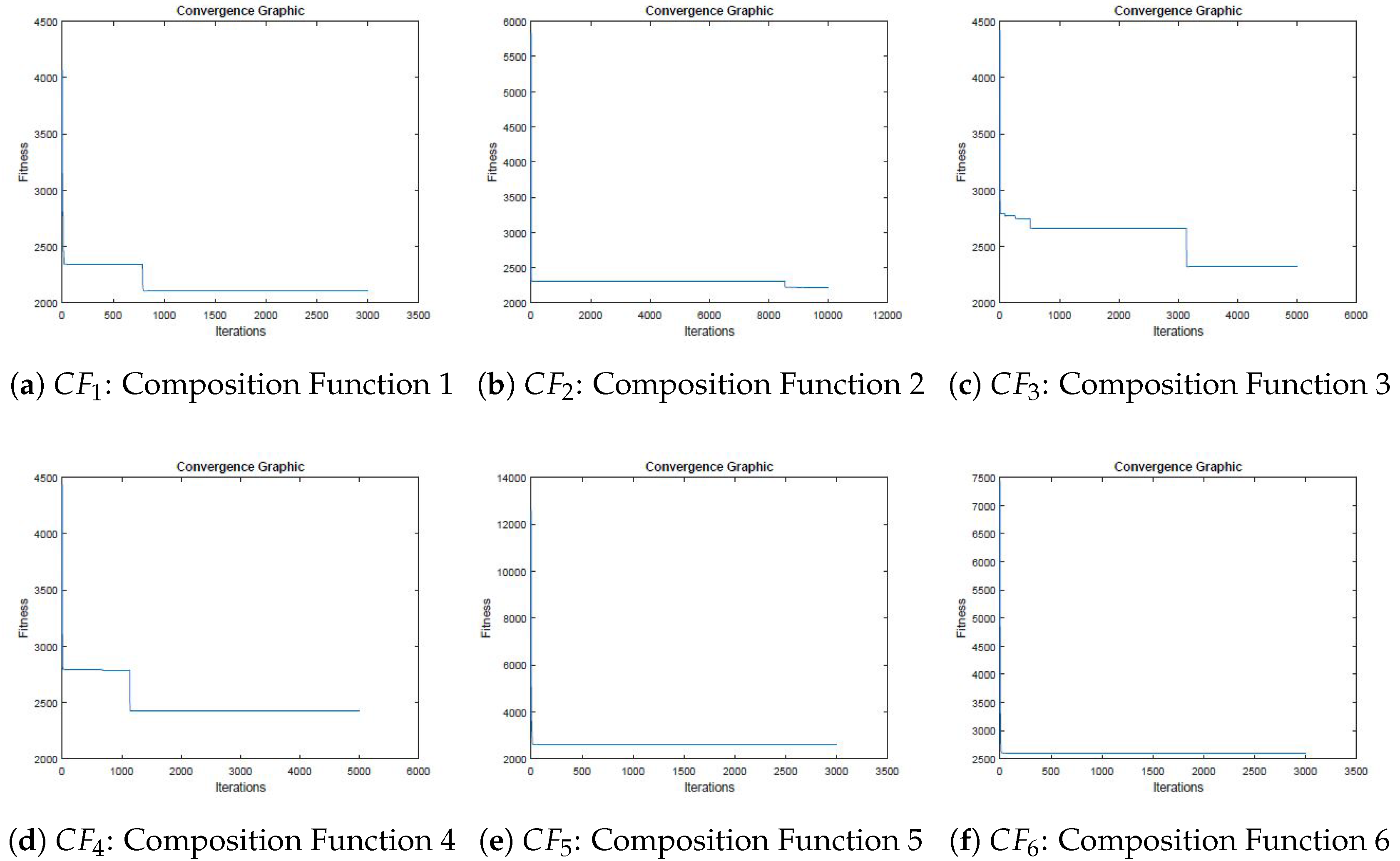Figure 19 shows the convergence graphics obtained by VLE for these benchmark functions. The number of iterations was fixed at 1000, 3000, 5000 and 10000 for these functions. 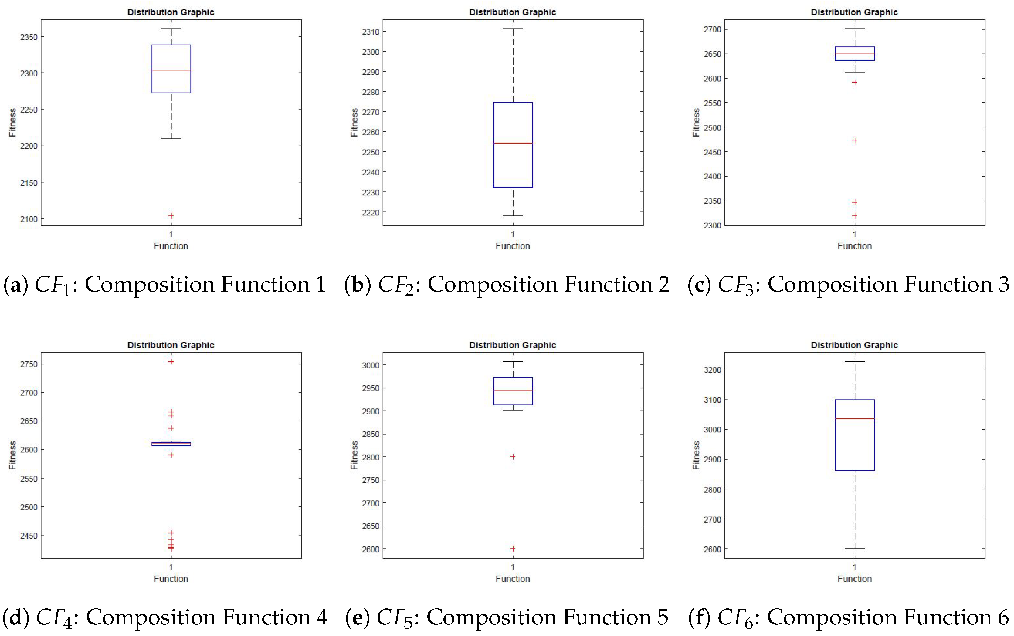Figure 20 shows the distribution graphics obtained by VLE for the composite functions chosen. All experiments were repeated at least 31 times to guarantee a meaningful statistical analysis.

7. Conclusions and Future Work

First, it is important to address the advantages and disadvantages of our algorithm. Regarding the advantages, we have the following: (1) VLE does not require special functions, such as a sigmoidal function, to incorporate variables in binary and discrete domains in addition to the variables in the real domain. This process is easy to do because the same source of inspiration allows it. The movements take place in a continuous space in which changes of states of thermodynamic equilibrium are made. In this space, the variables are converted into molar fractions of the liquid and gas phases (vapour), which vary between zero and one. This functionality will be implemented in the next version of VLE; (2) To determine the direction in which the next move will be made for each decision variable, VLE scans the current solution’s environment in opposite directions, the direction in which the decision variable increases and the direction in which it decreases. The change in the value of one of the variables is performed by holding the values of the other variables constant in the values corresponding to those of the current solution. Once the declining direction of fitness has been chosen, it is maintained until a new growth in fitness is observed; (3) The step size in the search space of the thermodynamic states is not constant, but in general, it is decreasing in both directions. Of course, the condition can also occur in which it decreases in one direction and increases in the other direction. In addition, the step size is different for each variable. All the above is due to the shape of the equilibrium curve of the binary system that represents the decision variable and the current location of the value of the variable between its limits or range of variation. Finally, the step size for each possible movement of a decision variable is established autonomously, also, due to the shape of the saturation curve; (4) The algorithm allows fine changes to be made around the value of each decision variable, close to a local optimum. This is because for each restart, once the movement is completed, VLE reduces the search ranges around the average value of the best values found for the decision variables. This reduction produces the same effect that is obtained when focusing and enlarging an image; (5) The researcher is not required to have any knowledge of the simulated physical-chemical phenomenon. In general, the researcher must specify the objective function, the penalty function for that function, the number of decision variables of the optimization problem, the number of executions to be carried out, the number of movements per execution, the minimum acceptable difference between the current value of the objective function and the best-found value so as not to become stuck in local optima, and the probability of acceptance of poor solutions. Regarding the disadvantages, we have the following: (1) Between one movement and the next, VLE performs $(\alpha -1)D$ evaluations of the objective function, D being the number of problem decision variables. In other words, VLE creates a population of $(\alpha -1)D$ solutions whose fitness must be evaluated. The greater the number of decision variables of the problem, the greater the memory used by VLE to perform the search and the greater the time it takes to perform an effective movement; (2) The determination of bubble and dew temperatures requires additional iterative calculations, which translates into an increase in computational cost. However, in this version, the calculations have been reduced to a minimum since they are carried out using the bisection numerical method. The use of this particular method also guarantees the determination of said temperatures; (3) Since it truly simulates the vapour-liquid equilibrium of binary mixtures that form ideal solutions, the search is restricted to the possible equilibrium states of the simulated system. This restriction, of course, can translate into a certain degree of loss of flexibility near a local optimum. At the least, disadvantages 2 and 3 will be eliminated in a future version of VLE.

Second, it is important to comment on and highlight the results obtained with our algorithm, applied to the fifteen classical reference functions, and compared with the corresponding results obtained by four well-known and robust optimization algorithms. As we said, the results were analysed using two techniques: (1) by performing a thorough comparative analysis of the average values obtained by each function and each metaheuristic; and (2) by using the root-mean-square error, or RMSE. Based on the first technique of analysis, we may say that VLE had competitive performance among PSO, GSA, DE, and WOA, with a weighted average performance of 44.83%, and that VLE occupied the third place among the five compared algorithms. Using the second technique of analysis, we may affirm that, in general, and in terms of datasets, the average dataset obtained by VLE is better adjusted to the true values of optimum values of the reference functions than any of the published data sets for PSO, GSA, DE, and WOA.

This analysis allows us first to corroborate that there is no metaheuristic that is more capable at solving optimization problems than any other metaheuristic and second, to say that to establish a significant difference among these algorithms, it is necessary to considerer a wider set of reference functions. This will be considered in future work.

According to the results obtained, we believe that the vapour-liquid equilibrium is a good idea as a source of inspiration to develop a novel and robust metaheuristic. In addition, we affirm that the search of a local optimal can also be performed by using simple mathematical models that simulate the phenomenon that has been the inspiration source of the algorithm.

As a future work, we would like to include more benchmark functions of the four types considered in this research. Furthermore, we will increase the number of dimensions from 30 to 50 and 100 to analyse the performance of the procedure with more decision variables. Additionally, we would like to transform the actual version of VLE (based on a single starting solution with multistart), into a swarm optimization algorithm. Finally, we would like to apply our algorithm for solving real-world optimization problems in the engineering area.