Detectability of Delamination in Concrete Structure Using Active Infrared Thermography in Terms of Signal-to-Noise Ratio

Abstract

Detecting subsurface delamination is a difficult and vital task to maintain the durability and serviceability of concrete structure for its whole life cycle. The aim of this work was to obtain better knowledge of the effect of depth, heating time, and rebar on the detectability capacity of delamination. Experimental tests were carried out on a concrete specimen in the laboratory using Long Pulsed Thermography (LPT). Six halogen lamps and a long wavelength infrared camera with a focal plane array of 640 × 480 pixels were used as the heat source and infrared detector, respectively. The study focused on the embedded imitation delaminations with the size of 10 cm × 10 cm × 1 cm, located at depths varying from 1 to 8 cm. The signal-to-noise ratio (SNR) was applied as a criterion to assess the detectability of delamination. The results of this study indicate that as the provided heating time climbed, the SNR increased, and the defect could be identified more clearly. On the other hand, when using the same heating regime, a shallow delamination displayed a higher SNR than a deeper one. The moderate fall of the SNR in the case of imitating defect located below reinforced steel was also observed. The absolute contrast was monitored to determine the observation time, and the nondimensional prefactor k was empirically proposed to predict the depth of delamination. The mean absolute percentage error (MAPE) was used to quantitatively evaluate the difference between forecasted and real depth, which evaluation confirmed the high reliability of the estimated value of the prefactor k.

1. Introduction

Durability and serviceability are important requirements for concrete structures over the whole of their service life. In reality, subsurface defects appear inside concrete structures, and are not noticed until they expose significant damage and failure. In developed countries, the cost of repair work ensuring acceptable operation conditions is even higher than the expense used to construct a new one [1,2]. Hence, the prediction and detection of defects is essential, and should be carefully studied, in order to determine the structural conditions, and propose suitable repair methods for potentially damaged structure.

Defects, such as crack, delamination, spalling, and air void, are primarily caused by the corrosion of embedded steel bars, successive freeze-thaw cycles, thermal effect, shrinkage, traffic load, or overloading, such as earthquake or heavy vehicles [3,4]. Delaminations formed mainly from invisible hidden cracks in structures are usually at the region above the upper reinforcement layer in the protective concrete layer, or even at the place between reinforcement layers, as shown in Figure 1 [5,6].

To detect and characterize delaminations in the concrete structures, various nondestructive techniques (NDTs) have been developed and applied. These NDTs include simple methods, such as chain dragging and hammer sounding, and other advanced methods, like ground penetrating radar (GPR), ultrasonic, and impact-echo [7]. All of them are available and suitable for the identification of delamination depths deeper than 5 to 10 cm [8].

It needs to be noted that the types of structure, loading conditions, environmental conditions, and diameter of steel bars have a strong effect on the design of the thickness of concrete cover [9,10,11]. According to AASHTO LRFD (2014) [9], the minimum required thickness of the concrete cover of bridge structures is about 50 mm in most cases, and approximately 75 mm in the case of coastal and cast-against-earth structures. As required in ACI 318-05 (2014) [10] for building structures, the concrete cover thickness is at least 20 mm for structure not exposed to the weather or in contact with the ground, and 76 mm for concrete permanently exposed to the earth.

Currently, among many NDTs, the active infrared thermography technique has been proven to be an effective tool to determine the location, and also the depth of delamination in concrete structures [6,11,12,13]. This technique gives reliable results in the evaluation of the near-surface region with the depth of defects less than 10 cm [8,14]. In several researches, when the ratio between the size and the depth of delamination (so-called width-to-depth ratio or WTDR) is smaller than 2.0, the delamination was considered undetectable [15,16], while other authors stated that delamination with a WTDR smaller than 2.0 could be detected using advanced image processing techniques, as discussed in Section 2 [3,6,11,17,18,19]. In this study, the Long Pulsed Thermography (LPT) technique, one of the most common methods of active infrared thermography, is used to clarify the effects of depth, heating time, and steel bars on the detectability capacity of delamination inside a concrete specimen.

In the present work, a series of experimental tests were carried out on a concrete specimen containing artificial delaminations of different sizes and depths, which create different WTDRs. Reinforcements are located above several delaminations having depth ranging from 5 to 8 cm, as mentioned in Section 4.1. The signal-to-noise ratio (SNR) criterion is applied to assess the detectability of delamination using active infrared thermography. A delamination can be considered as “detectable” when the SNR has a value higher than zero [20,21,22]. In addition, the absolute contrast of each delamination is monitored to determine the observation time, propose the nondimensional prefactor k, and predict the depth of delamination.

2. Related Works

Pulsed thermography is a well-known NDT to detect defects in concrete structures. In this method, the surface of the structure is heated up by external heat sources, such as infrared radiators, halogen lamps, or flash lamps [23,24]. The surface temperature of structure in both heating time and cooling time is analyzed to determine and characterize delamination in LPT [25]. The absolute contrast is usually used to detect delamination, while the depth of defects is quantitatively computed by using the linear relationship between the depth square and observation time [16]. Section 5.1 will discuss in detail the definition of absolute contrast and observation time. Several studies relating the above-mentioned methods are presented as follows.

In 2002, Maierhofer et al. [26] carried out an experimental test on two concrete specimens using three infrared radiators with 7200 watts of total energy. Eight artificial delaminations with sizes of 20 cm × 20 cm × 10 cm and 10 cm × 10 cm × 10 cm by polystyrene were implemented inside the specimen. The radiators were moved vertically on a line array with a fixed distance of 15 cm, and they concluded that a big delamination at a depth of 10 cm (with WTDR of 2.0) could be identified. In addition, using impulse thermography to detect voids in four concrete slabs with dimensions of 100 cm × 100 cm × 30 cm was conducted by Maierhofer et al. in 2007 [17]. Defects were simulated by the inclusion of polystyrene cuboids or integration of gas concrete parts with sizes of 10 cm × 10 cm × 5 cm. The defect depths were 6 and 10 cm, and the heating duration varied between 5 and 30 min. One, two, and three layers of reinforcement mats were embedded inside a specimen. This work was studied on the influence of concrete age, pore content, aggregate type, and reinforcement density on the detectability of shallow voids. In all cases, the void at a depth of 6 cm was detected (with WTDR of about 1.67). The results showed that the reinforcement density has only a slight influence on the detectability of subsurface defects. Furthermore, in 2008, Cheng et al. [19] carried out empirical research using an IR camera NEC TH7102 (Tokyo, Japan) with minimum detectable temperature difference of 0.08 °C. Four halogen lamps were used to produce uniform heat flux. The authors concluded that it was difficult to identify the defect with the smallest size (5 cm × 5 cm) at the largest cover thickness of 3 cm.

The applicability and limits of void and delamination detection in concrete structures using infrared thermography was performed by Patricia Cotic et al. in 2015 [18]. They conducted experiments of 51 artificially defects with sizes from 1.2 to 10 cm located at depths from 0.5 to 12.5 cm in concrete, using active infrared thermography. The heating time was from 5 to 30 minutes. The study mentioned that it was possible to detect defects with the ratio between depth-and-size ≤ 0.9 and 1.3, when using the thermal contrast and phase contrast methods, respectively. A 3-dimensional numerical simulation of the thermal transfer occurring in concrete specimens containing defects was also performed. The relationship between the depth of defect and maximum time, as well as maximum frequency, was determined. Based on that, the depth of defects in concrete structures could be predicted. In addition, the research works of Ahlborn in 2015 [3] and Vaghefi in 2013 [6] showed that all five delaminations placed deeper than 5.72 cm (2.25 in), or with a WTDR < 1.33, were undetectable. In these studies, a 1500watt infrared heater placed at 1.1 m and a FLIR SC640 camera (FLIR, USA) located at 1.7 m from the specimen surface were used. All artificial delaminations had the same sizes of 7.62 cm × 7.62 cm × 0.95 cm or 3 in × 3 in × 3/8 in.

In the IRT field, the SNR has been demonstrated as a highly effective criterion in judging the detectability of defects. This criterion was used in many previous studies for several materials, not only for concrete, but also for steel, composite, and carbon fiber (CFRP) [11,20,21,22,27,28,29]. In 2010, Madruga et al. [27] conducted the IRT test for a carbon fiber reinforced plastic specimen and 25 Teflon squares with five different sizes located at five different depths. In this study, they applied the SNR to distinguish defects that were detectable and undetectable. Their results showed that delaminations with the sizes of 3, 5, and 10 cm at a depth ≥0.4, 0.6, and 1.0 mm, respectively, were not detected. In 2013 Usamentiaga et al. [29] carried out a test on a CFRP specimen of aeronautical structure using SNR to compare the excitation (i.e., optical pulse, step heating, and ultrasound) and image postprocessing methods (polynomial fit, first and second derivatives, phase of the Discrete Fourier Transform, Skewness, and Kurtosis). For concrete structure, Tran et al. (2018) [11] conducted an experimental study on a concrete specimen in the laboratory using the PT and Pulse Phase Thermography (PPT) methods. In this study, they used SNR to investigate the detectability of delaminations with WTDRs ranging from 1.0 to 7.9. The results showed that a combination of PT and PPT could be used to detect delaminations with a WTDR ≥ 1.25. The SNR criterion was also studied to detect the defects in other materials, such as carbon fiber and plexiglas by Hidalgo-Gato et al. in 2013 [20] and reinforced honeycomb sandwich panels by R. Usamentiaga et al. in 2012 [28].

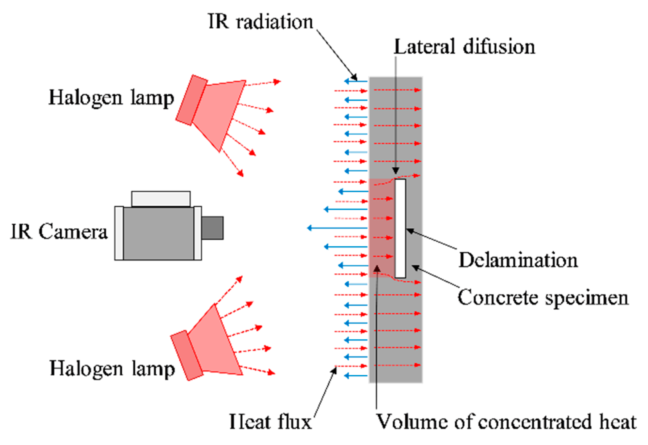
3. Fundamental of Infrared Thermography

In the IRT technique, an IR camera is used to measure the infrared radiation emitted from the structure surface, which then it is converted into the temperature. The total radiation energy received by IR camera (W_tot) includes the emission from the object (W₁), the reflected emission from ambient sources (W₂), and the emission from the atmosphere (W₃), as shown in Equation (1) and in Figure 2 [12,30,31].

$$W_{tot}=W_1+W_2+W_3,$$

(1)

where, W₁, W₂, and W₃ are calculated from Equations (2)–(4), respectively [12,30,31].

$$W_1=\tau \times \epsilon \times \sigma \times T_{obj}^4,$$

(2)

$$W_2=\tau \times \left(1-\epsilon \right)\times \sigma \times T_{amb}^4,$$

(3)

$$W_3=\left(1-\tau \right)\times \sigma \times T_{atm}^4,$$

(4)

where, ε is the emissivity of the object, τ is the transmittance of the atmosphere, σ is the Stefan–Boltzmann constant (σ = 5.67 × 10⁻⁸ W m⁻² K⁻⁴), (1 − ε) is the reflectance of the object, (1 − τ) is the emissivity of the atmosphere, T_obj is the temperature of an object, T_abm is the reflected temperature (from ambient sources), and T_atm is the atmosphere temperature. Substituting Equations (2)–(4) in (1), Equation (5) is obtained. Therefore, the object temperature can be determined using Equation (6).

$$W_{tot}=W_1+W_2+W_3=\tau \times \epsilon \times \sigma \times T_{obj}^4+\tau \times \left(1-\epsilon \right)\times \sigma \times T_{amb}^4+\left(1-\tau \right)\times \sigma \times T_{atm}^4,$$

(5)

$$T_{obj}=\sqrt[4]{\frac{W_{tot}-\tau \times \left(1-\epsilon \right)\times \sigma \times T_{amb}^4-\left(1-\tau \right)\times \sigma \times T_{atm}^4}{\tau \times \epsilon \times \sigma }},$$

(6)

It should be noted that the values of ε, τ, T_refl, and T_atm must be set up in the camera as initial parameters. The surface temperature of the object is automatically computed by the IR camera from Equation (6). In this study, the reflected temperature is considered equal to the ambient temperature as discussed in our previous study [12]. The emissivity of material is influenced by the type of material, surface, geometry, observation direction, wavelength, and temperature [32]. For example, the emissivity of the concrete of 0.92 can be used for a wide range of spectrum from 2 to 20 µm, while it is around 0.974 for concrete pavement tested in the wavelength band of 6 to 20 µm, and around 0.95 for dry concrete tested under temperature of 36 °C with the wavelength varying from 2 to 5 µm [33]. In this study, the specimen was heated including an electrical tape piece glued on the surface. The temperature on the piece of electrical tape with known emissivity was employed to measure the surface emissivity of the concrete specimen. Thus, the value of measured emissivity of approximately 0.95 is set as a constant value during each test case.

4. Experimental Design and Procedure

4.1. Preparation of the Test Specimen

A concrete slab was fabricated with design compression strength of 30 MPa. Square pieces of polystyrene were used to simulate horizontal artificial delaminations inside the specimen, because of its similar thermal conductivity to air [6]. Eight artificial cuboids have the same sizes of 10 cm × 10 cm × 1 cm. The depth of defects ranges from 1 to 8 cm, and the WTDR varies from 1.25 to 10.

Table 1. The data of delaminations inside the concrete specimen.

Delamination	Size (cm × cm × cm)	Depth (cm)	Width-to-Depth Ratio (WTDR)	Location in Comparison with Steel Bars	Testing Face
BD1	10 × 10 × 1	4.0	2.50	Above	Back
BD2	10 × 10 × 1	3.0	3.30	Above	Back
BD3	10 × 10 × 1	2.0	5.00	Above	Back
BD4	10 × 10 × 1	1.0	10.0	Above	Back
BD5	10 × 10 × 1	4.0	2.50	Above	Back
BD6	10 × 10 × 1	3.0	3.30	Above	Back
BD7	10 × 10 × 1	2.0	5.00	Above	Back
BD8	10 × 10 × 1	1.0	10.0	Above	Back
FD1	10 × 10 × 1	5.0	2.00	Above	Front
FD2	10 × 10 × 1	6.0	1.67	Above	Front
FD3	10 × 10 × 1	7.0	1.43	Above	Front
FD4	10 × 10 × 1	8.0	1.25	Above	Front
FD5	10 × 10 × 1	5.0	2.00	Below	Front
FD6	10 × 10 × 1	6.0	1.67	Below	Front
FD7	10 × 10 × 1	7.0	1.43	Below	Front
FD8	10 × 10 × 1	8.0	1.25	Below	Front

lists the data of the artificial delaminations. The horizontal delamination is called “delamination” in the following sections.

Figure 3 shows the arrangement of artificial delaminations inside the concrete specimen. Steel bars with a diameter of 10 mm are placed above the defects at the cross-section B–B, whereas no rebar is arranged at the cross-section A–A. The goal of this arrangement is to consider and evaluate the effects of rebars on the detectability of deep defects with low WTDRs. The test was conducted on both faces of the specimen to assess the delaminations with a range of concrete cover from 1 to 8 cm. In Table 1, the letters “F” and “B” indicate the test for the front and back face, respectively. In this study, the experimental test was conducted in the laboratory to minimize the wind effect. The side faces of the specimen were covered by polystyrene plates to reduce the thermal loss during the heating and cooling period of the test.

4.2. Testing Process

Six halogen lamps (500 watts per each lamp) with 3000 watts of total output energy were used as the heat source to heat the specimen surface. The heat source was mounted on a steel frame at a distance of 1.2 m from the surface of the specimen. Figure 4 shows the system of infrared thermography in the laboratory.

In every test case, the ambient temperature and relative humidity were measured using the Kestrel 3000 (Figure 4c), of which the accuracy of temperature is 0.1 °C and of relative humidity is 0.1% [34]. In active IRT, out of several factors (i.e., emissivity, reflected temperature, and distance from the camera to the specimen surface), the ambient temperature and relative humidity are two initial parameters that are set to the IR camera as the input data. These two input parameters are assumed as constant values during each test case and shown in

Table 2. Environmental conditions for each case of the test.

Heating Time (min)	Test Case	Back Face (Depth from 1 to 4 cm)		Front Face (Depth from 5 to 8 cm)
		Ambient Temperature (°C)	Relative Humidity (%)	Ambient Temperature (°C)	Relative Humidity (%)
2	Case 1	19.9	63	-	-
3	Case 1	18.4	59	-	-
	Case 2	20.8	91	-	-
	Case 3	19.7	64	-	-
4	Case 1	20.6	94	-	-
	Case 2	21.2	86	-	-
	Case 3	17.7	62	-	-
5	Case 1	20.1	77	-	-
	Case 2	18.2	55	-	-
	Case 3	17.9	84	-	-
10	Case 1	18.9	69	-	-
	Case 2	16.9	56	-	-
	Case 3	21.4	73	-	-
15	Case 1	24.2	85	10.2	59
	Case 2	24.8	61	-	-
	Case 3	17.1	66	-	-
20	Case 1	24.4	85	14.6	73
	Case 2	19.2	57	17.1	53
	Case 3	18.0	76	15.8	74
25	Case 1	24.5	86	12.9	35
	Case 2	24.5	58	14.2	78
	Case 3	21.2	73	16.1	63
30	Case 1	24.3	79	12.1	48
	Case 2	25.2	53	13.7	83
	Case 3	17.7	84	16.8	62
40	Case 1	-	-	15.9	52
	Case 2	-	-	15.4	77

. The IR camera will automatically calculate the atmosphere transmission and the surface temperature of the specimen [30]. It is noted that a small amount of data of this study can be found in our previous research work [5].

The specimen was heated uniformly in five heating regimes of 15, 20, 25, 30, and 40 min for the front face (depths of 5 to 8 cm), and nine cases of 2, 3, 4, 5, 10, 15, 20, 25, and 30 min for the back face (depths of 1 to 4 cm). After heating, all lamps were turned off, and the surface temperature in both heating and cooling duration was measured by a long wavelength IR thermal camera (FLIR SC660). With recording intervals of 10 s, thermal images were taken by the IR detector, which was fixed on a tripod at a distance of 3.3 m from the specimen surface, and at an unchanged height of 78 cm from the ground (the height of the camera was nearly the same level as the center of the specimen).

Table 3. Technical data of the FLIR SC660 camera [35].

Items	Parameters
IR resolution	(640 × 480) pixels
Field of view (FOV)	(24° × 18°)/0.3 m
Thermal sensitivity/NETD	<30 mK @ + 30 °C
Spatial resolution (IFOV)	0.65 mrad
Wavelength	(7.5–13) µm
Focal Plane Array (FRA) sensor	Uncooled microbolometer
Temperature range	(−40–+120) °C
Accuracy	±1 °C or ±1% of reading

shows the technical data of the IR camera [35].

5. Analysis of Experimental Results

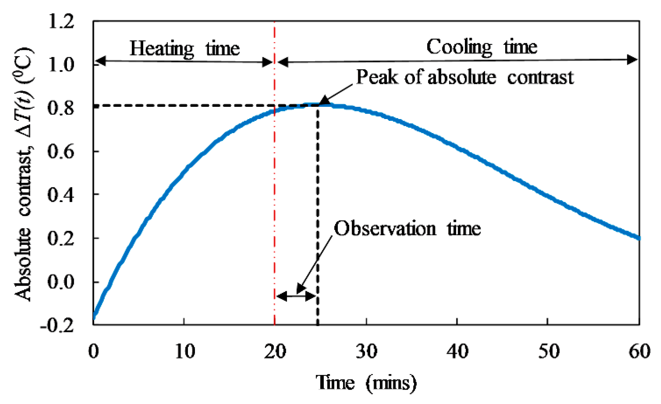
5.1. Signal-to-Noise Ratio (SNR) Criterion and Absolute Contrast Method

The SNR has been used to distinguish the detectability or undetectability of delaminations. The positive or negative values indicate that the delamination is detected or undetected, respectively [11,20,21,22,27,36]. The SNR represents the contrast between the surface temperature above a defective area and its surroundings (in dB) [20]. Therefore, the degree of SNR shows the visibility level of delamination in concrete structures. The higher the SNR, the more clearly the delamination can be observed. The SNR can be determined by using Equation (7) [20,36]:

$$SNR(dB)=\frac{S}{N}=20{\log }_{10}\left(\frac{abs\left(S_{-}area-N_{-}area\right)}{{\sigma }_{noise}}\right),$$

(7)

$${\sigma }_{noise}=\sqrt{\frac{1}{n-1}{{\displaystyle \sum _{i=1}^n\left(x_i-\overline{x}\right)}}^2},$$

(8)

where, $S_{-}area$ and $N_{-}area$ are the average surface temperature of the signal and noise areas, respectively. The signal and the noise areas are the regions above a defect and its neighborhood correspondingly. ${\sigma }_{noise}$ is the standard deviation of the surface temperature of the noise area.

For using long pulse thermography, the problem of nonuniform heating is unavoidable. In addition, the effects of environmental conditions on the surface temperature of the specimen during both heating and cooling duration always exist. Therefore, the noise area is chosen to ensure that the effects of nonuniform heating and environment are minimal. For these reasons, the noise area is proposed as the perimeter around the imitating deterioration, whereas the signal area is the region above the delamination. In previous studies, the perimeter of noise has been demonstrated more effectively than cases of one point or group of three points [3,12,37,38]. In this study, all artificial delaminations have the same sizes of 10 cm × 10 cm × 1 cm, so both signal and noise areas are selected with the same dimensions for each defect to have consistent parameters. Signal area and noise area are expressed using the red square and the blue square, respectively, as shown in Figure 5.

The heat flux conducting in the concrete specimen is interrupted by defects, because the thermal conductivity of the defect (the air) is much less than that of the concrete. Consequently, the heat flux is slowed down and concentrated above delaminations during heating [39]. After the heat source (halogen lamps) is switched off, at the region surrounding delamination, the heat flux continues transferring without the obstruction from the heated face to the opposite face of the specimen, while it cannot transmit significantly through the delamination, and the concentrated thermal energy on the surface of the defect reflects to the surface at the same side of the heat source. Therefore, the surface temperature above a delamination is higher than its neighborhood solid area. Figure 6 illustrates the heat transfer mechanism using halogen lamps.

In this method, absolute contrast and observation time are the two main parameters that are used for defining the visibility of the delamination, and predicting the delamination’s depth. The absolute contrast (∆T(t)) is defined as the difference between the average temperature above a defect and its surroundings, while the observation time (T_max) is the duration from when the time of the heat source was turned off to the peak of the absolute contrast curve [16].

$$\Delta T\left(t\right)=T_d\left(t\right)-T_{Sa}\left(t\right),$$

(9)

where, T_d(t) and T_Sa(t) are the mean values of surface temperature within a defect area and reference area, respectively. Therefore, absolute contrast is a function of time, t.

In this study, T_d(t) is the average surface temperature of signal area, whereas T_Sa(t) is the average temperature on the perimeter of the noise area. Figure 5 shows the signal and noise areas. The absolute contrast curve is plotted, and then the observation time is determined as shown in Figure 7. Figure 7 is a case of 20 min of heating for the depth of 2 cm. It should be noted that in the case that the observation time cannot be identified, it is impossible to predict the depth of a delamination [3].

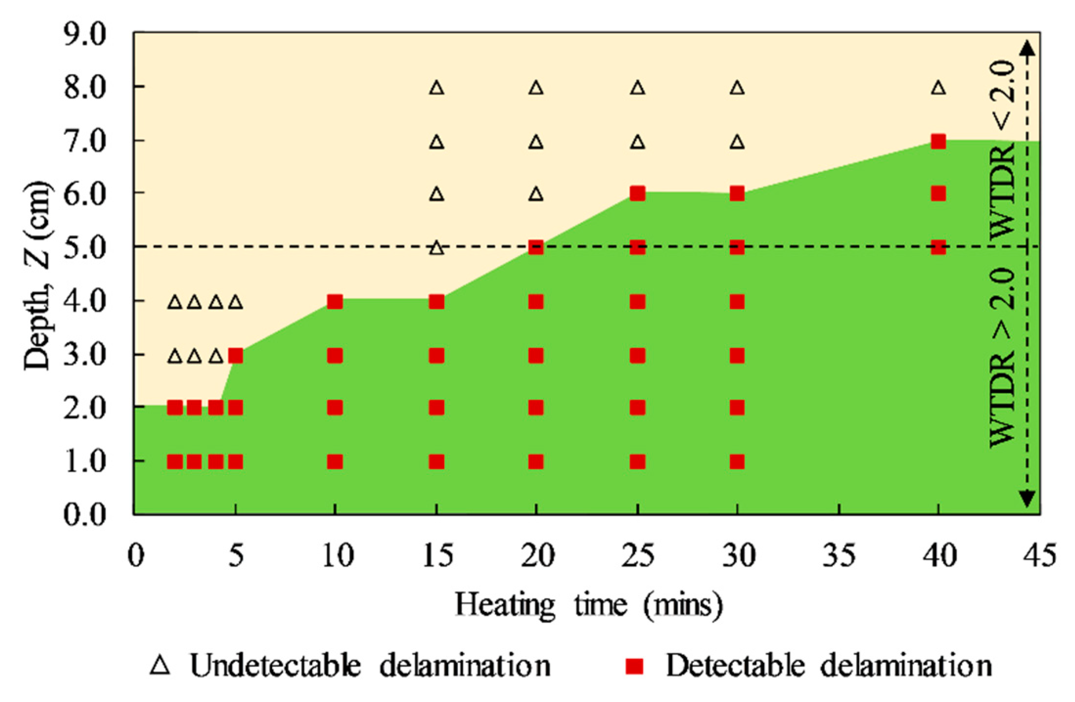
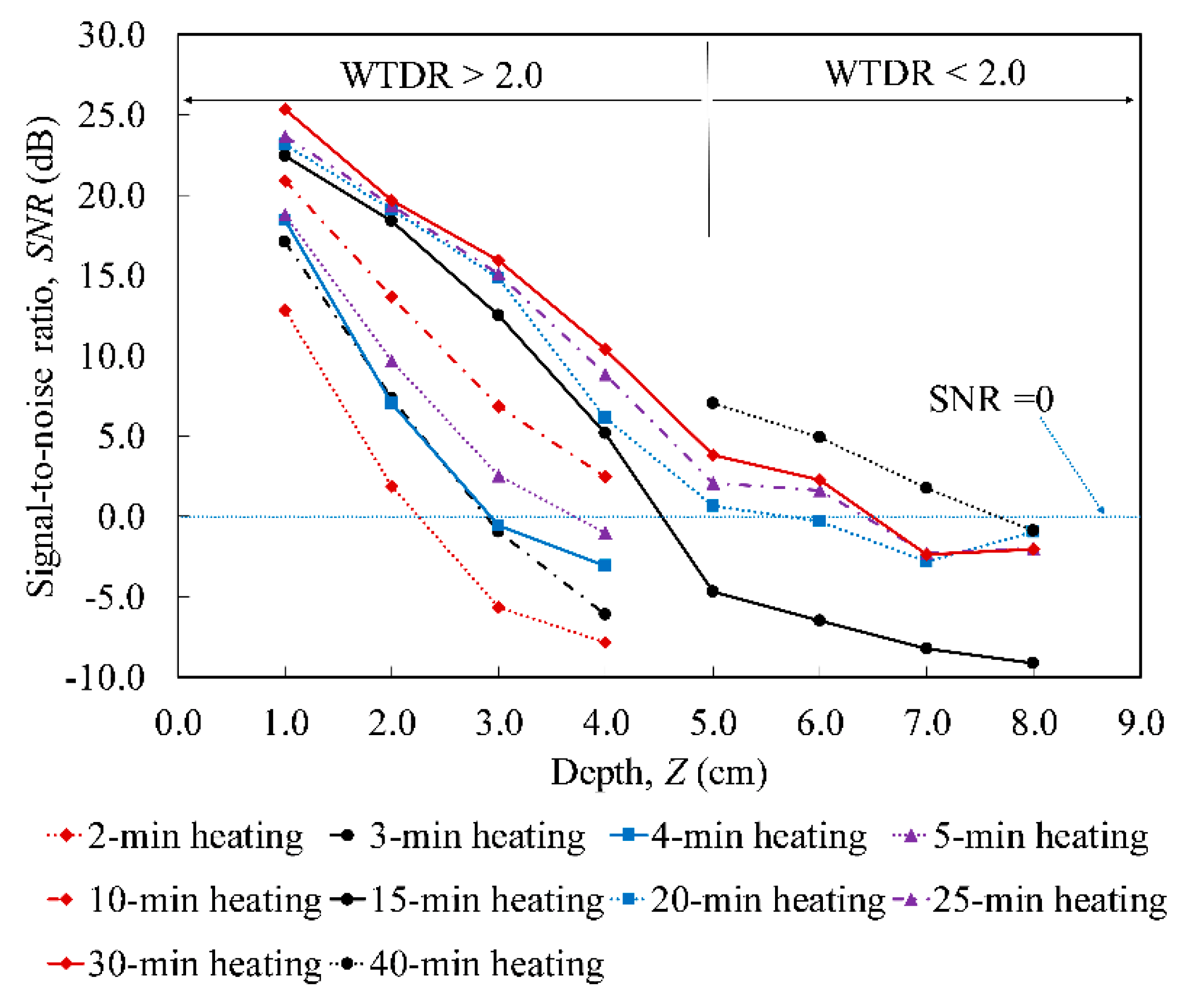
5.2. Detectability of Delaminations Using SNR

Figure 8a shows an example of the thermal image of the back face of the specimen with delamination depths ranging (1 to 4) cm. The image is taken at 1000 s after turning off the heat source under 30 min heating. The yellow (bright) and green (dark) colors represent high and low temperature, respectively. Delamination can be clearly recognized, because the surface temperature above a defect is much higher than its surroundings. Figure 8b shows the temperature profile of line 1–1 illustrated in Figure 8a. This line crosses from left to right of the thermal image, cutting the four upper delaminations. It can be stated that under the same testing conditions, the surface temperature above the deeper delamination is smaller than that above a shallower one.

By using the SNR shown in Equation (7), the image contrast (or the detectability) is measured with different heating regimes, as summarized in

Table 4. The mean value of SNR in heating regime cases.

Heating Time (min)	BD4 (Depth 1 cm)	BD3 (Depth 2 cm)	BD2 (Depth 3 cm)	BD1 (Depth 4 cm)	FD1 (Depth 5 cm)	FD2 (Depth 6 cm)	FD3 (Depth 7 cm)	FD4 (Depth 8 cm)
	SNR (dB)	SNR (dB)	SNR (dB)	SNR (dB)	SNR (dB)	SNR (dB)	SNR (dB)	SNR (dB)
2	12.88	1.90	−5.62	−7.81	-	-	-	-
3	17.12	7.35	−0.93	−6.11	-	-	-	-
4	18.48	7.05	−0.52	−3.06	-	-	-	-
5	18.81	9.72	2.57	−0.98	-	-	-	-
10	20.88	13.67	6.89	2.47	-	-	-	-
15	22.42	18.38	12.53	5.18	−4.65	−6.51	−8.19	−9.11
20	23.18	19.09	14.85	6.15	0.67	−0.32	−2.82	−0.92
25	23.67	19.38	15.09	8.87	2.10	1.62	−2.30	−1.97
30	25.34	19.69	15.92	10.41	3.86	2.31	−2.38	−2.06
40	-	-	-	-	7.08	4.94	1.78	−0.87

. The results show that as depth increases, the specimen needs to be heated for much longer. For example, delaminations at 1 and 2 cm depths were detected quickly after just 2 min of heating, while it required 5 and 10 min heating to detect delaminations at 3 and 4 cm depths, respectively. In the case of the deeper delaminations from 5 to 8 cm, the required heating time increased significantly. For example, to identify the delaminations with depths of 5 and 6 cm, FD1, WTDR = 2.0 and FD2, WTDR ≈ 1.67, respectively, the specimen needed to be heated corresponding to 20 and 25 min, while the heat source had to be kept on for 40 min for a depth of 7 cm (FD3, WTDR ≈ 1.43). The deepest delamination, i.e., FD4 (WTDR = 1.25) at 8 cm depth, was undetectable, even when heated up to 40 min. The results indicated that infrared thermography makes it possible to detect the delamination with WTDR ≥1.43. Based on Table 4, the detectability of delaminations can be divided into two regions of negative and positive SNR values as illustrated in Figure 9. The green (dark) and pale-yellow (bright) regions depict the identified and unidentified delaminations, respectively. The triangular symbols with black borders represent the undetectable delaminations, while the red squares stand for the detectable delaminations.

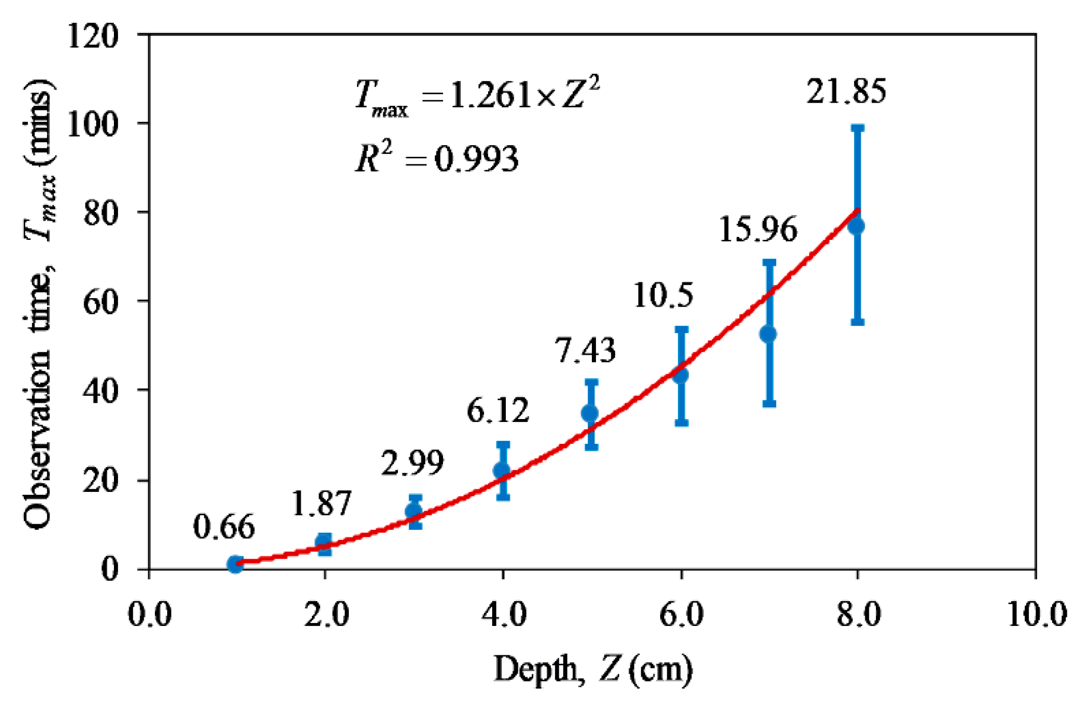
5.3. Effects of Depth on the Detectability of Delaminations

Figure 10 shows the mean values of the SNR of ten different heating regimes. In the graph, the blue horizontal dotted line separates two regions, in which data points above this line represent detectable delaminations, while the other points under the line indicate undetectable delaminations.

Overall, the same general tendency can be observed in all cases of heating time. SNR decreases quickly with the increase of depth, except for defects located at 8 cm depth, which indicate no tendency. It can be observed that the image contrast drops significantly against the depth of shallow delaminations, while it changes gradually with deep delaminations. For example, considering the 30 min heating regime, the SNR decreases by around 14.9 dB for the depth from 1 to 4 cm, whereas SNR is just 5.9 dB for the depth from (5 to 8) cm.

On the other hand, shallower deteriorations show more clearly and easily than deeper ones. The heat flux reflects quickly back to the surface, and produces a high signal of contrast, whereas a larger volume of concentrated heat above a deeper delamination diffuses in many directions [39]. This leads to reducing the thermal contrast. For example, the SNR in the heating case of 30 min varies from approximately 25.3 to 2.3 dB, corresponding to the defect depths increasing from 1 to 6 cm.

Figure 11 shows the SNR during cooling duration. Fifth-order polynomial fit curves were applied to reduce the noise, and illustrate the tendencies more clearly. For example, four SNR curves of the delaminations from 1 to 4 cm in Figure 11 show the same tendency. After the heat sources are turned off, the SNR curves increase and reach a peak, before dropping. Figure 11 also demonstrates the effects of depth on the detectability of delamination by using the SNR. The peak value of the SNR indicates the best observation of subsurface delamination.

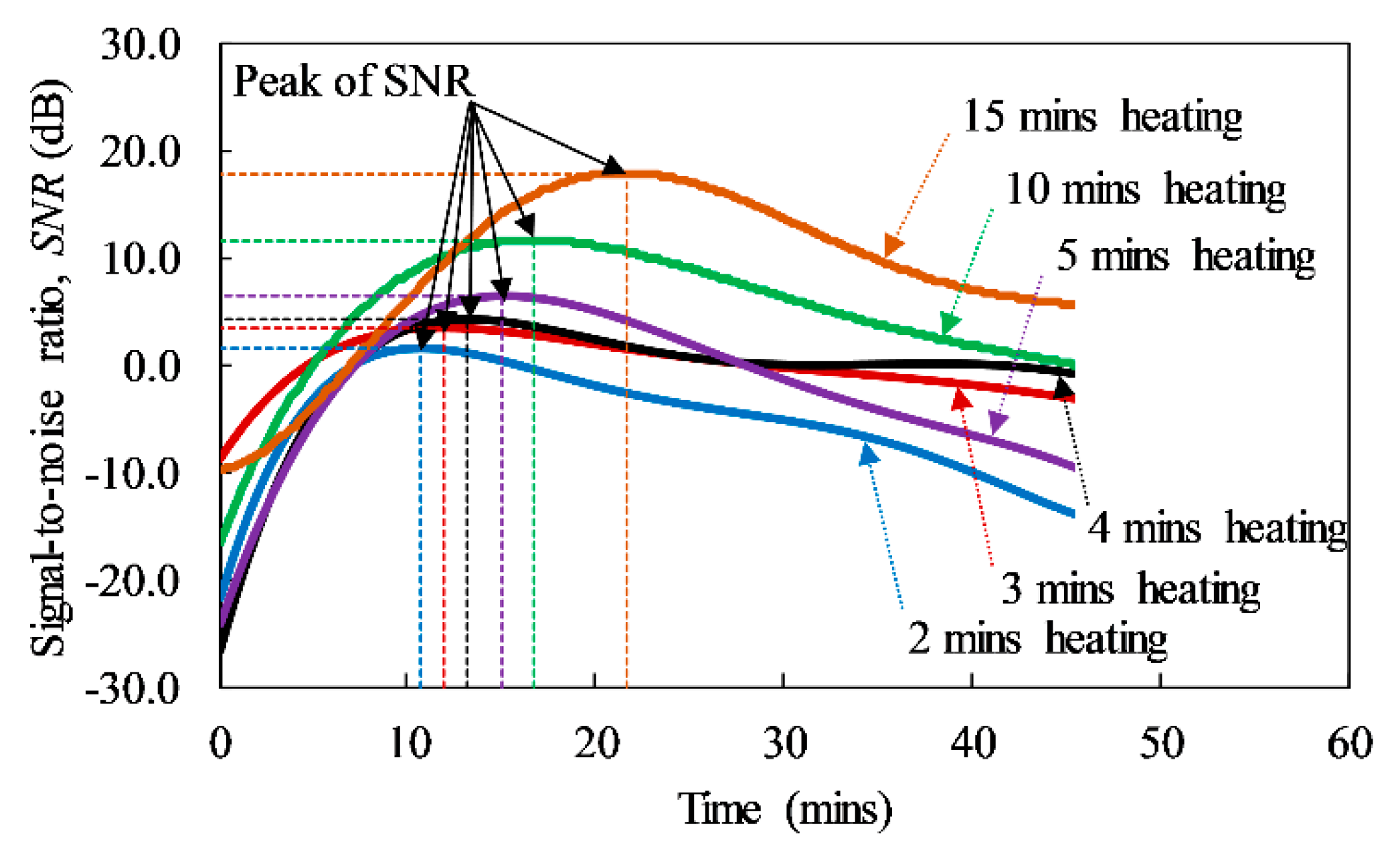
5.4. Effects of Heating Regime on the Detectability of Delaminations

Figure 12 depicts the SNR for all cases of different depths. On the graph, eight lines represent the mean values of SNR corresponding to the eight depths under ten heating regimes from 2 to 40 min. Generally, as the heating time increases, SNR climbs. The larger heating time means that more heat energy is provided to heat the specimen. With the same depth, the strength of volume concentrated heat produced in a longer heating time will be higher than in a shorter regime.

For the depths from 1 to 4 cm, the heat source energy significantly affects the thermal contrast, even when the specimen is stimulated by a short heating time (i.e., from 2 to 5 min). In particular, in the case of 4 cm depth, the SNR increases by approximately 8 dB within only 3 min from 2 to 5 min heating time, as shown in Figure 12. However, the SNR value increases only approximately 12.5 dB as the specimen heats up from 5 to 30 min. In addition, over a 15 min heating time, the SNR rises steadily at slow speed; for example, when the heating time goes up from 20 to 30 min for delamination at 2 cm depth, SNR increases from just 19.1 to 19.7 dB. In addition, for the depth from 5 to 8 cm, when the heating time increases from 15 to 20 min, SNR values go up quickly, but only delamination at 5 cm depth can be detected, while the others are still undetectable. From the heating time of over 20 min, delaminations at 5 and 6 cm depth show the same tendency, whereas delaminations at 7 and 8 cm depth do not show any tendency, and they are difficult to recognize by the naked eye. As the specimens continue heating up to 40 min, the 7 cm depth delamination shows better contrast with the SNR of about 1.8 dB, while the SNR value of delamination at 8 cm depth is still in the negative. The reason might be because the delamination at 8 cm depth has its WTDR of 1.25, which is usually reported as being unable to be detected [3,6,17,19].

Figure 13 shows an example of recorded SNR values for the 2 cm of defect depth in both heating and cooling time. Six heating regimes from 2 to 15 min are shown. Figure 13 also illustrates the effects of heating time on the detectability of defects. The same tendency can be observed in all SNR curves that the SNR climbs, even though the heat source is already turned off, and reaches the maximum value, before slumping.

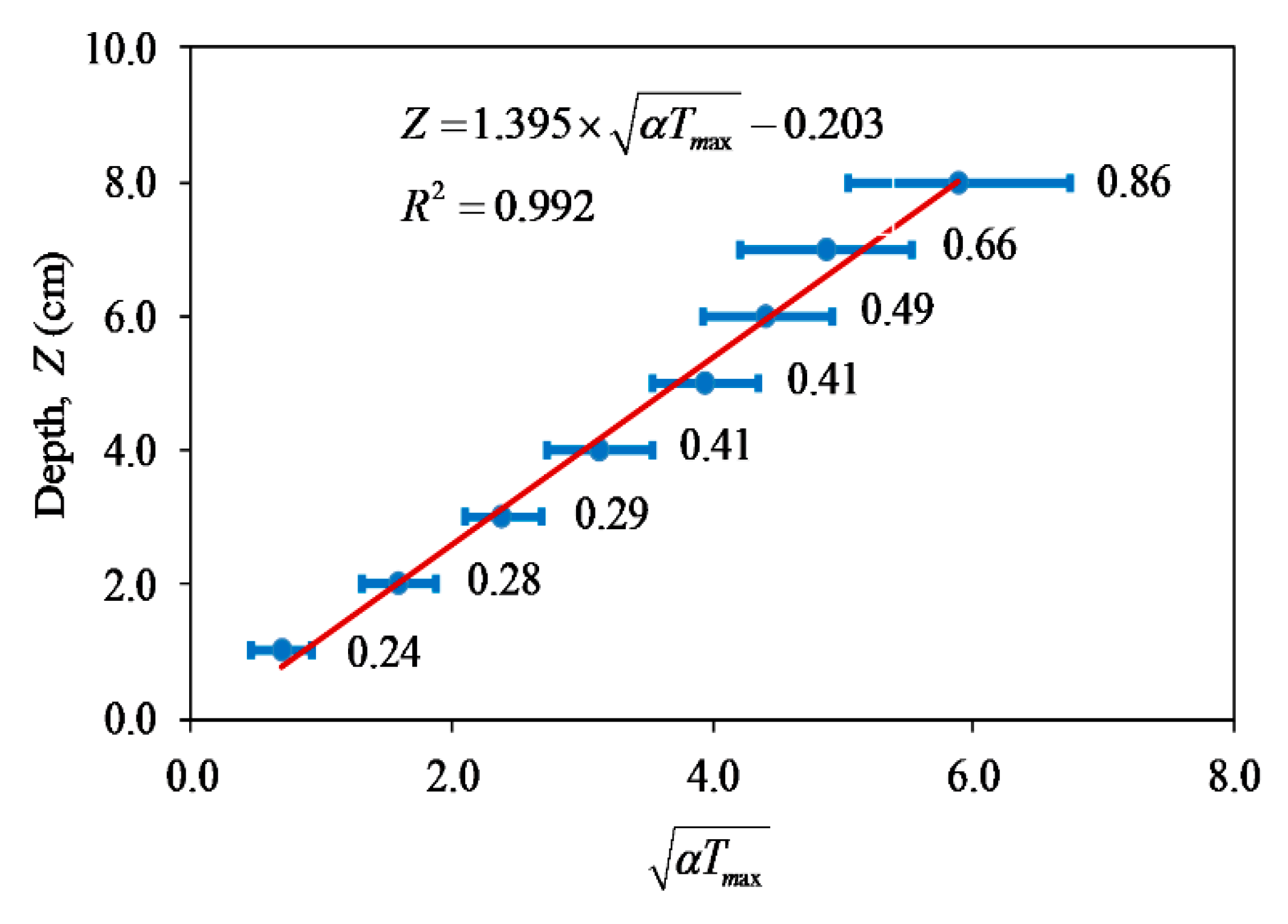
5.5. Estimation of the Nondimensional Prefactor for Depth Evaluation

Based on the theory of the one-dimensional propagation of heat, the observation time (T_max) is a quadratic function of the depth of delamination (Z) [15,40]. In this experimental study, this relationship is verified by plotting out the mean values of observation time in all cases of heating regimes with the real depth of delamination, as shown in Figure 14. The results of the statistical data analysis indicate that Equation (10) can be a quadratic function, with the coefficient of determination R² of 0.993 proving high reliability of the dataset.

$$T_{\max }=1.261\times Z^2,$$

(10)

It is noted that even though the SNR for the delamination with the depth of 8 cm is always of negative value, the peak of absolute contrast is still possible to observe. Therefore, the case of depth 8 cm is considered in estimating the nondimensional prefactor k.

In addition, as demonstrated in Figure 14, the shallower the delamination is located, the smaller the standard deviation of observation time that is obtained. In particular, they vary from about 0.7 to 21.9 min for 1 to 8 cm depth, respectively.

When the specimen is heated by a heat source, the transfer rate of heat of the specimen from the hot side to cold side is measured by the thermal diffusivity (α), which is the thermal conductivity divided by the density and specific heat capacity at constant pressure [16]. Thus, the relationship between observation time (T_max) and depth of defect (Z) can be expressed by the following equation [18].

$$Z=k\sqrt{\alpha T_{\max }},$$

(11)

where, k is a nondimensional prefactor used to forecast the depth of delaminations, which is presented in Section 5.6. In this study, to estimate the k values corresponding to a wide range of the thermal diffusivity (α), the α values were divided into fifteen values ranging from (6.8 to 8.2) × 10⁻⁷ m² s⁻¹ [41] with the same interval of 0.1 × 10⁻⁷ m² s⁻¹. The relationship between Z and $\sqrt{\alpha T_{\max }}$ in Equation (11) was analyzed, and the linear function was used to fit the data. Thus, the factor k could be estimated as the slope of the linear regression.

The results showed that the factor k decreased from 1.414 to 1.288 when the thermal diffusivity increased from (6.8 to 8.2) × 10⁻⁷ m² s⁻¹. Figure 15 shows an example of the relationship mentioned in Equation (11) under the mean value of thermal diffusivity α = 7.5 × 10⁻⁷ m² s⁻¹. The fitting linear regression function is shown in Equation (12), which has a very good fitness, with R² = 0.992. The intercept is now set equal to zero to achieve a new equation, $Z=1.347\times \sqrt{\alpha T_{\max }}$ and factor k can be obtained as 1.347. It should be noted that Cotic et al., in 2015, proposed nondimensional prefactor, k = 1.8 based on numerical simulation using α = 7.5 × 10⁻⁷ m² s⁻¹. These results are different with those from our experimental study which might be due to the assumption of uniform heating, homogenous material and without heat flux through the side faces of the specimen.

$$Z=1.395\times \sqrt{\alpha T_{\max }}-0.203,$$

(12)

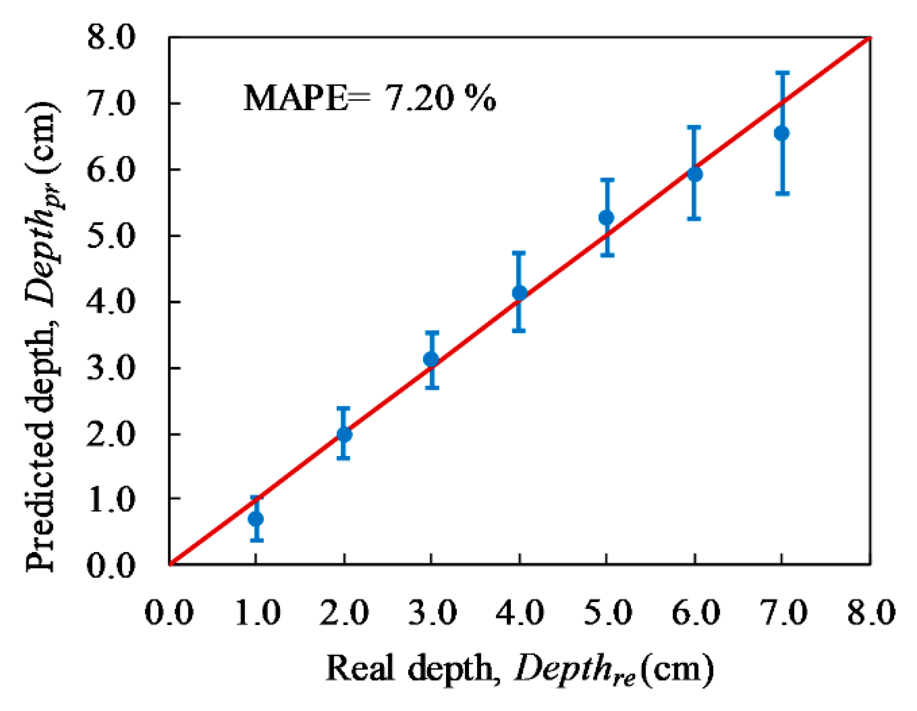
5.6. Prediction of the Depth of Delaminations

The depths of delaminations are predicted by using the linear regression with the chosen values of thermal diffusivity (e.g., using Equation (12) in the case of α = 7.5 × 10⁻⁷ m² s⁻¹). The mean absolute percentage error (MAPE) is commonly used to measure the differences between two datasets [42]; thus, it was applied in this study to assess the difference between the predicted depth and the real depth of defects. The MAPE can be defined by using Equation (13).

$$MAPE(\%)=\frac{1}{N}{\displaystyle \sum _{i=1}^N\left|\frac{Dept{h}_{pr}-Dept{h}_{re}}{Dept{h}_{re}}\right|}\times 100,$$

(13)

where, the Depth_re is the real depth, Depth_pr is the predicted depth, and N is the total number of assessed values.

The MAPEs obtained from fifteen different cases of thermal diffusivity from (6.8 to 8.2) × 10⁻⁷ m² s⁻¹ are almost similar to 7.20%. MAPE less than 10% indicates a good agreement between the expected and real depths as categorized by Lewis, as shown in

Table 5. Classification of the accuracy of forecasted data based on the mean absolute percentage error (MAPE) [42].

MAPE	The Accuracy of Forecasted Data
<10%	very good
<20%	good
<30%	reasonable
>30%	inaccurate

[42].

Figure 16 shows an example of the comparison between real and expected depths with the mean value of thermal diffusivity α = 7.5 × 10⁻⁷ m² s⁻¹. As depicted in Figure 16, a deeper delamination has a higher value of standard deviation of the depth than a shallower one; they range from approximately 0.34 to 0.92 cm, corresponding to depths of 1 to 7 cm.

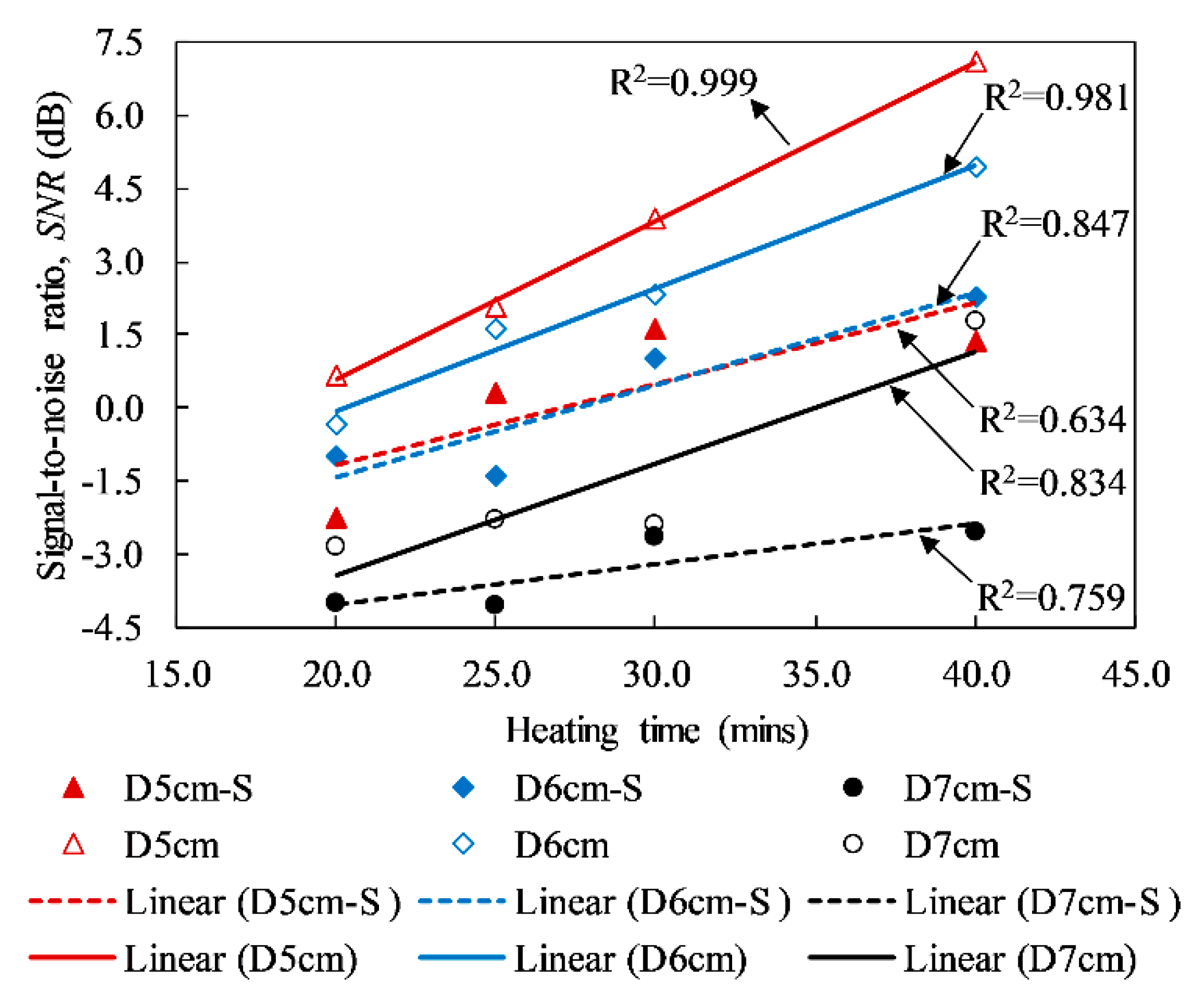
5.7. Effects of Steel Bars on the Detectability of Delaminations

Figure 17 shows the influence of steel bars in terms of SNR. It is noted that delaminations at 8 cm depth were undetectable, so they are not included in Figure 17. Linear regression is used to fit the data. In Figure 17, “D5 cm” represents the delamination at 5 cm depth without steel bars, while “D5cm-S” represents the case having steel bars. For the depths of 6 and 7 cm, they indicate the same manner as the depth of 5 cm. The results show that with the same depth, heating time, and test conditions, the SNR obtained in cases without reinforcement is higher than cases with steel bars. This means that the delaminations under reinforced steel can be observed less clearly than those without the effect of reinforcement. Besides, the heating time provided for detecting delaminations requires a longer duration due to the influence of steel bars. For example, the delaminations at 5 and 6 cm depth without the effect of rebars can be detected under only 20 and 25 min heating regimes, respectively, while those placed below rebars are undetectable corresponding to the SNRs of −2.24 and −1.40 for 5 and 6 cm depths, respectively. Even for heating up to 40 min, the delamination at 7 cm depth below rebars was still undetectable.

6. Conclusions

In this study, experimental tests were conducted on a concrete slab using the Long Pulsed Thermography technique. Halogen lamps were used as the heat source. Eight square artificial delaminations of the same size were implemented at different known depths. In addition, reinforcement steel was also embedded inside the specimen. The main goals of this study were to assess the detectability capacity of delamination in terms of SNR, propose the nondimensional prefactor k, predict the depth of delamination, and evaluate the effects of steel bars on the identification ability of defects. The following conclusions were achieved in this study.

Active infrared thermography is an effective tool applied in nondestructive testing for the detectability of delamination. The delamination with concrete cover up to 7 cm in concrete structures can be identified successfully using SNR criterion.

The SNR decreases moderately with an increase of delamination depth. On the other hand, the longer the heating time, the higher the SNR that can be obtained. It should be noted that in this study, the delamination with the depth of 8 cm was not identified.

The nondimensional prefactor k was determined from the quadratic relationship between the depth of delamination and the observation time under chosen thermal diffusivities. The difference between depths expected from the estimated empirical prefactor k and real depths was approximately 7.20%, which proved the reliability of the estimated value of the prefactor.

The effects of steel bars indicate that the SNR of a delamination above reinforcement is significantly higher than those under rebar. This means that defects located below reinforced steel are more difficult to detect than those above rebar.

References

1. Abdel-Qader, I.; Yohali, S.; Abudayyeh, O.; Yehia, S. Segmentation of thermal images for non-destructive evaluation of bridge decks. NDT E Int. 2008, 41, 395–405. [Google Scholar] [CrossRef]
2. Milovanović, B.; Banjad Pečur, I. Detecting Defects in Reinforced Concrete using the Method of Infrared Thermography. CrSNDT J. 2013, 3, 3–13. [Google Scholar]
3. Ahlborn, T.M.; Brooks, C.N. Evaluation of Bridge Decks Using Non-Destructive Evaluation (NDE) at Near Highway Speeds for Effective Asset Management; RC-1617; Michigan Technological University: Houghton, MI, USA, 30 June 2015. [Google Scholar]
4. Portland Cement Association. Types and Causes of Concrete Deterioration; Portland Cement Association: Skokie, IL, USA, 2002. [Google Scholar]
5. Tran, Q.H.; Huh, J.; Mac, V.H.; Kang, C.; Han, D. Effects of rebars on the detectability of subsurface defects in concrete bridges using square pulse thermography. NDT E Int. 2018. [Google Scholar] [CrossRef]
6. Vaghefi, K. Infrared Thermography Enhancements for Concrete Bridge Evaluation. Ph.D. Thesis, Michigan Technological Univesity, Houghton, MI, USA, 2013. [Google Scholar]
7. Hiasa, S.; Birgul, R.; Watase, A.; Matsumoto, M.; Mitani, K.; Catbas, F.N. A Review of Field Implementation of Infrared Thermography as a Non-destructive Evaluation Technology Shuhei. In Proceedings of the Sixth Annual International Conference on Computing in Civil and Building Engineering, Orlando, FL, USA, 17 June 2014; pp. 455–462. [Google Scholar]
8. Milovanović, B.; Banjad Pečur, I. Review of Active IR Thermography for Detection and Characterization of Defects in Reinforced Concrete. J. Imaging 2016, 2, 11. [Google Scholar] [CrossRef]
9. American Association of State Highway Transportation Officials. AASHTO LRFD Bridge Design Specifications; American Association of State Highway Transportation Officials: Washington, DC, USA, 2014. [Google Scholar]
10. American Concrete Institute. Building Code Requirements for Structural Concrete (ACI 318M-14); American Concrete Institute: Farmington Hills, MI, USA, 2014. [Google Scholar]
11. Tran, Q.H.; Huh, J.; Kang, C.; Lee, B.Y.; Kim, I.T.; Ahn, J.H. Detectability of Subsurface Defects with Different Width-to-Depth Ratios in Concrete Structures Using Pulsed Thermography. J. Nondestruct. Eval. 2018, 37, 32. [Google Scholar] [CrossRef]
12. Huh, J.; Tran, Q.H.; Lee, J.-H.; Han, D.; Ahn, J.-H.; Yim, S. Experimental Study on Detection of Deterioration in Concrete Using Infrared Thermography Technique. Adv. Mater. Sci. Eng. 2016, 2016, 1053856. [Google Scholar] [CrossRef]
13. Wysocka-Fotek, O.; Oliferuk, W.; Maj, M. Reconstruction of size and depth of simulated defects in austenitic steel plate using pulsed infrared thermography. Infrared Phys. Technol. 2012, 55, 363–367. [Google Scholar] [CrossRef]
14. Maierhofer, C.; Arndt, R.; Röllig, M.; Rieck, C.; Walther, A.; Scheel, H.; Hillemeier, B. Application of impulse-thermography for non-destructive assessment of concrete structures. Cem. Concr. Compos. 2006, 28, 393–401. [Google Scholar] [CrossRef]
15. Vavilov, V.; Taylor, R. Theoretical and Practical Aspects of the Thermal Nondestructive Testing of Bonded Structures. In Research Techniques in NDT; Sharpe, R.S., Ed.; Academic Press: London, UK, 1982; Volume 5, pp. 238–279. [Google Scholar]
16. Maldague, X.P.V. Nondestructive Evaluation of Materials by Infrared Thermography; Springer: London, UK, 1993; ISBN 9781447119975. [Google Scholar]
17. Maierhofer, C.; Arndt, R.; Röllig, M. Influence of concrete properties on the detection of voids with impulse-thermography. Infrared Phys. Technol. 2007, 49, 213–217. [Google Scholar] [CrossRef]
18. Cotič, P.; Kolarič, D.; Bosiljkov, V.B.; Bosiljkov, V.; Jagličić, Z. Determination of the applicability and limits of void and delamination detection in concrete structures using infrared thermography. NDT E Int. 2015, 74, 87–93. [Google Scholar] [CrossRef]
19. Cheng, C.C.; Cheng, T.M.; Chiang, C.H. Defect detection of concrete structures using both infrared thermography and elastic waves. Autom. Constr. 2008, 18, 87–92. [Google Scholar] [CrossRef]
20. Hidalgo-Gato, R.; Andrés, J.R.; Lopez-Higuera, J.M.; Madruga, F.J. Quantification by Signal to Noise Ratio of Active Infrared Thermography Data Processing Techniques. Opt. Photonics J. 2013, 3, 20–26. [Google Scholar] [CrossRef]
21. Larsen, C.A. Document Flash Thermography. Ph.D. Thesis, Utah State University, Logan, UT, USA, 2011. [Google Scholar]
22. Svantner, M.; Muzika, L.; Chmelík, T.; Skala, J.; Švantner, M.; Muzika, L.; Chmelík, T.; Skála, J. Quantitative evaluation of active thermography using contrast-to-noise ratio. Appl. Opt. 2018, 57, D49–D55. [Google Scholar] [CrossRef] [PubMed]
23. Almond, D.P.; Pickering, S.G. An analytical study of the pulsed thermography defect detection limit. J. Appl. Phys. 2012, 111, 093510. [Google Scholar] [CrossRef] [Green Version]
24. Weritz, F.; Arndt, R.; Röllig, M.; Maierhofer, C.; Wiggenhauser, H. Investigation of concrete structures with pulse phase thermography. Mater. Struct. 2005, 38, 843–849. [Google Scholar] [CrossRef]
25. Maldague, X.; Marinetti, S. Pulse phase infrared thermography. J. Appl. Phys. 1996, 79, 2694–2698. [Google Scholar] [CrossRef] [Green Version]
26. Maierhofer, C.; Brink, A.; Röllig, M.; Wiggenhauser, H. Transient thermography for structural investigation of concrete and composites in the near surface region. Infrared Phys. Technol. 2002, 43, 271–278. [Google Scholar] [CrossRef]
27. Madruga, F.J.; Albendea, P.; Ibarra-Castanedo, C.; López-Higuera, J.M. Signal to Noise Ratio (SNR) Comparison for Lock-in Thermographic Data Processing Methods in CFRP Specimen. In Proceedings of the 10th International Conference on Quantitative Infrared Thermography, Québec, QC, Canada, 27–30 July 2010. [Google Scholar]
28. Usamentiaga, R.; Venegas, P.; Guerediaga, J.; Vega, L.; López, I. Non-destructive inspection of drilled holes in reinforced honeycomb sandwich panels using active thermography. Infrared Phys. Technol. 2012, 55, 491–498. [Google Scholar] [CrossRef]
29. Usamentiaga, R.; Venegas, P.; Guerediaga, J.; Vega, L.; López, I. A quantitative comparison of stimulation and post-processing thermographic inspection methods applied to aeronautical carbon fibre reinforced polymer. Quant. Infrared Thermogr. J. 2013, 10, 55–73. [Google Scholar] [CrossRef]
30. FLIR System Inc. The Ultimate Infrared Handbook for R & D Professionals; FLIR System Inc.: Hong Kong, China, 2012. [Google Scholar]
31. Usamentiaga, R.; Venegas, P.; Guerediaga, J.; Vega, L.; Molleda, J.; Bulnes, F. Infrared Thermography for Temperature Measurement and Non-Destructive Testing. Sensors 2014, 14, 12305–12348. [Google Scholar] [CrossRef] [PubMed] [Green Version]
32. Vollmer, M.; Möllmann, K.-P. Infrared Thermal Imaging: Fundamentals, Research and Applications; WILEY-VCH Verlag GmbH & Co. KGaA: Weinheim, Germany, 2010; ISBN 978-3-527-40717-0. [Google Scholar]
33. MICRO-EPSILON. Basics of Non Contact Temperature Measurement; MICRO-EPSILON: Raleigh, NC, USA, 2018. [Google Scholar]
34. Nielsen-Kellerman. Instruction Manual of Kestrel 3000 ™ ®; Nielsen-Kellerman: Chester, PA, USA, 1999. [Google Scholar]
35. FLIR System Inc. FLIR SC660 Catalog: Technical Data of FLIR SC660 Infrared Camera; FLIR System Inc.: Hong Kong, China, 2014. [Google Scholar]
36. Albendea, P.; Madruga, F.J.; Cobo, A.; López-Higuera, J.M. Signal to Noise Ratio (SNR) Comparison for Pulsed Thermographic Data Processing Methods Applied to Welding Defect Detection. In Proceedings of the 10th International Conference on Quantitative Infrared Thermography, Québec, QC, Canada, 27–30 July 2010. [Google Scholar]
37. Brown, J.R.; Hamilton, H.R. Heating Methods and Detection Limits for Infrared Thermography Inspection of Fiber-Reinforced Polymer Composites. ACI Mater. J. 2007, 104, 481–490. [Google Scholar]
38. Tran, Q.H.; Han, D.; Kang, C.; Haldar, A.; Huh, J. Effects of Ambient Temperature and Relative Humidity on Subsurface Defect Detection in Concrete Structures by Active Thermal Imaging. Sensors 2017, 17, 1718. [Google Scholar] [CrossRef] [PubMed]
39. Kretzmann, J.E. Evaluating the Industrial Application of Non-Destructive Inspection of Composites Using Transient Thermography. Ph.D. Thesis, University of Stellenbosch, Stellenbosch, South Africa, 2016. [Google Scholar]
40. Maldague, X.P.V. Applications of Infrared Thermography in Nondestructive Evaluation; Elsevier: Lausanne, Switzerland, 2000; pp. 591–609. ISBN 978-0080430201. [Google Scholar]
41. Maldague, X.P. Theory and Practice of Infrared Technology for Nondestructive Testing; John Wiley & Sons, Inc.: New York, NY, USA, 2001. [Google Scholar]
42. Lewis, C.D. Demand Forecasting and Inventory Control: A Computer Aided Learning Approach; Woodhead Publishing Ltd.: Cambridge, UK, 1997; ISBN 9781855732414. [Google Scholar]
Figure 1. Location of delamination in concrete structures.
Applsci 08 01986 g001
Figure 2. The principle of infrared thermography.
Applsci 08 01986 g002
Figure 3. Arrangement of artificial delaminations inside the concrete specimen.
Applsci 08 01986 g003
Figure 4. System of infrared thermography and equipment: (a) System of infrared thermography; (b) FLIR SC660 IR Camera (FLIR, Wilsonville, OR, USA); and (c) Kestrel 3000 (Nielsen-Kellerman, Chester, PA, USA).
Applsci 08 01986 g004
Figure 5. Selection of S a r e a and N a r e a for signal-to-noise ratio (SNR) calculation.
Applsci 08 01986 g005
Figure 6. The heat transfer mechanism using halogen lamps.
Applsci 08 01986 g006
Figure 7. Absolute contrast curve in the case of 20 min heating for delamination at 2 cm depth.
Applsci 08 01986 g007
Figure 8. The test results at 1000 s after turning off the heat source in the case of 30-min heating: (a) thermal image and (b) the surface temperature profile of the line 1–1.
Applsci 08 01986 g008
Figure 9. Partition of the undetectability and detectability of delaminations in the tests.
Applsci 08 01986 g009
Figure 10. SNR for delaminations with different depths.
Applsci 08 01986 g010
Figure 11. SNR during cooling time for the depth from (1 to 4) cm in the case of 30-min heating.
Applsci 08 01986 g011
Figure 12. The SNR for delaminations under different heating times.
Applsci 08 01986 g012
Figure 13. The SNR during both cooling time and heating time for 2 cm of depth under 2 to 15 min heating.
Applsci 08 01986 g013
Figure 14. The relationship between the depth and observation time.
Applsci 08 01986 g014
Figure 15. The relationship between α T max and the depth (Z) in the case of α = 7.5 × 10⁻⁷ m2 s−1.
Applsci 08 01986 g015
Figure 16. Comparison between the real and predicted depths of delaminations in the case of α = 7.5 × 10⁻⁷ m2 s−1.
Applsci 08 01986 g016
Figure 17. Comparison of the SNR of cases without and with steel bars.
Applsci 08 01986 g017