Effective Implementation of Edge-Preserving Filtering on CPU Microarchitectures

Abstract

In this paper, we propose acceleration methods for edge-preserving filtering. The filters natively include denormalized numbers, which are defined in IEEE Standard 754. The processing of the denormalized numbers has a higher computational cost than normal numbers; thus, the computational performance of edge-preserving filtering is severely diminished. We propose approaches to prevent the occurrence of the denormalized numbers for acceleration. Moreover, we verify an effective vectorization of the edge-preserving filtering based on changes in microarchitectures of central processing units by carefully treating kernel weights. The experimental results show that the proposed methods are up to five-times faster than the straightforward implementation of bilateral filtering and non-local means filtering, while the filters maintain the high accuracy. In addition, we showed effective vectorization for each central processing unit microarchitecture. The implementation of the bilateral filter is up to 14-times faster than that of OpenCV. The proposed methods and the vectorization are practical for real-time tasks such as image editing.

1. Introduction

Edge-preserving filters [1,2,3,4,5] are the basic tools for image processing. The representatives of the filters include bilateral filtering [1,2], non-local means filtering [3] and guided image filtering [4,5,6]. These filters are used in various applications, such as image denoising [3,7], high dynamic range imaging [8], detail enhancement [9,10,11], free viewpoint image rendering [12], flash/no-flash photography [13,14], up-sampling/super resolution [15,16], alpha matting [5,17], haze removal [18], optical flow and stereo matching [19], refinement processing in optical flow and stereo matching [20,21] and coding noise removal [22,23].

The kernel of the edge-preserving filter can typically be decomposed into range and/or spatial kernels, which depend on the difference between the value and position of reference pixels. Bilateral filtering has a range kernel and a spatial kernel. Non-local means filtering has only a range kernel. The shape of the spatial kernel is invariant across all pixels. By contrast, that of the range kernel is variant; thus, the range kernel is computed adaptively for each pixel. The adaptive computation is expensive.

Several acceleration algorithms have been proposed for the bilateral filtering [8,24,25,26,27,28,29,30,31,32] and non-local means filtering [24,30,33,34]. These algorithms reduce the computational order of these filters. The order of the naïve algorithm is $O(r^2)$, where r is the kernel radius. The order of the separable approximation algorithms [24,25] is $O(r)$, and that of constant-time algorithms [27,28,29,30,31,32,33,34,35,36] is $O(1)$. The separable approach is faster than the naïve; however, the approximation accuracy is low. The constant-time algorithms are faster than the $O(r^2)$ and $O(r)$ approaches in large kernel cases. In the case of multi-channel image filtering with intermediate-sized kernels, the method tends to be slower than the naïve algorithms owing to the curse of dimensionality [27], which indicates that the computational cost increases exponentially with increasing dimensions. Furthermore, when the kernel radius is small, the naïve algorithm can be faster than the algorithms of the order $O(r)$ or $O(1)$ owing to the offset times, which refers to pre-processing and post-processing such as creating intermediate images. In the present study, we focus on accelerating the naïve algorithm of the edge-preserving filtering based on the characteristics of computing hardware.

The edge-preserving filter usually involves denormalized numbers, which are special floating-point numbers defined in IEEE Standard 754 [37]. The definition of the denormalized numbers is discussed in Section 3. The formats are supported by various computing devices, such as most central processing units (CPUs) and graphics processing units (GPUs). The denormalized numbers represent rather small values that cannot be expressed by normal numbers. Although the denormalized numbers can improve arithmetic precision, their format is different from the normal numbers. Therefore, the processing of the denormalized numbers incurs a high computational cost [38,39,40]. The edge-preserving filters have small weight values, where a pixel is across an edge. The values tend to be the denormalized numbers. Figure 1 shows the occurrence of the denormalized numbers in various edge-preserving filtering. The denormalized numbers do not influence the eventual results, because these values are almost zero in the calculations. Hence, we can compute edge-preserving filtering with high-precision even by omitting the denormalized numbers. Moreover, the omission would be critical for accelerating the edge-preserving filtering.

A fast implementation requires effective utilization of the functionalities in CPUs and GPUs. In the present study, we focus on a CPU-centric implementation. Existing CPU microarchitectures are becoming complex. The architectures are based on multi-core architectures, complicated cache memories and short vector processing units. Single-instruction, multiple-data (SIMD) [41] instruction sets in vector processing units are especially changed. The evolution of the SIMD instructions has taken the form of the increased vector length [42], increased number of types of instructions and decreased latency of instructions. Therefore, it is essential to use SIMD instructions effectively for extracting CPU performance. In the edge-preserving filtering, execution of the weight calculation is the main bottleneck. Thus, the vectorization for weight calculation has a significant effect.

In the present study, we focus on two topics: the influence of denormalized numbers and effective vectorized implementation on CPU microarchitectures in the edge-preserving filtering. For the first, we verify the influence of the denormalized numbers on the edge-preserving filtering, and then, we propose methods to accelerate the filter by removing the influence of the denormalized numbers. For the second, we compare several types of vectorization of bilateral filtering and non-local means filtering. We develop various implementations to clarify suitable representations of the latest CPU microarchitectures for these filters.

The remainder of this paper is organized as follows. In Section 2, we review bilateral filtering, non-local means filtering and their variants. Section 3 describes IEEE standard 754 for floating point numbers and denormalized numbers. In Section 4, we present CPU microarchitectures and SIMD instruction sets. We propose novel methods for preventing the occurrence of the denormalized numbers in Section 5. In Section 6, we introduce several types of vectorization. Section 7 presents our experimental results. Finally, in Section 8, we show a few concluding remarks.

2. Edge-Preserving Filters

General edge-preserving filtering in finite impulse response (FIR) filtering is represented as follows:

$$\begin{array}{c}\hfill \mathit{J}(\mathit{p})=\frac{1}{\eta }\sum _{\mathit{q}\in \mathcal{N}(\mathit{p})}f(\mathit{p},\mathit{q})\mathit{I}(\mathit{q}),\end{array}$$

(1)

where $\mathit{I}$ and $\mathit{J}$ are the input and output images, respectively. $\mathit{p}$ and $\mathit{q}$ are the present and reference positions of pixels, respectively. A kernel-shaped function $\mathcal{N}(\mathit{p})$ comprises a set of reference pixel positions, and it varies for every pixel $\mathit{p}$. The function $f(\mathit{p},\mathit{q})$ denotes the weight of position $\mathit{p}$ with respect to the position $\mathit{q}$ of the reference pixel. $\eta$ is a normalizing function. If the gain of the FIR filter is one, we set the normalizing function as follows:

$$\begin{array}{c}\hfill \eta =\sum _{\mathit{q}\in \mathcal{N}(\mathit{p})}f(\mathit{p},\mathit{q}).\end{array}$$

(2)

Various types of weight functions are employed in edge-preserving filtering. These weights are composed of spatial and range kernels or only a range kernel. The weight of the bilateral filter is expressed as follows:

$$\begin{array}{ccc}\hfill f(\mathit{p},\mathit{q})& :=& \exp (\frac{{\parallel \mathit{p}-\mathit{q}\parallel }_2^2}{-2{\sigma }_s^2})\exp (\frac{{\parallel \mathit{I}(\mathit{p})-\mathit{I}(\mathit{q})\parallel }_2^2}{-2{\sigma }_r^2}),\hfill \end{array}$$

(3)

where ${\parallel ·\parallel }_2$ is the L2 norm and ${\sigma }_s$ and ${\sigma }_r$ are the standard deviations of the spatial and the range kernels, respectively. The weight of the non-local means filter is as follows:

$$\begin{array}{ccc}\hfill f(\mathit{p},\mathit{q})& :=& \exp (\frac{{\parallel \mathit{v}(\mathit{p})-\mathit{v}(\mathit{q})\parallel }_2^2}{-h^2}),\hfill \end{array}$$

(4)

where $\mathit{v}(\mathit{p})$ represents a vector, which includes a square neighborhood of the center pixel $\mathit{p}$. h is a smoothing parameter. The weight of the bilateral filter is determined by considering the similarity between the color and spatial distance between a target pixel and that of the reference pixel. The weight of the non-local means filter is defined by computing the similarity between the patch on the target pixel and that on the reference pixel. The weight of the non-local means filter is similar to the range weight of the bilateral filter for a multi-channel image.

To discuss the influence of the denormalized numbers, we introduce two variants of the bilateral and non-local means filters, namely the Gaussian range filter and the bilateral non-local means filter. The weight of the Gaussian range filter is expressed as follows:

$$\begin{array}{ccc}\hfill f(\mathit{p},\mathit{q})& :=& \exp (\frac{{\parallel \mathit{I}(\mathit{p})-\mathit{I}(\mathit{q})\parallel }_2^2}{-2{\sigma }_r^2}).\hfill \end{array}$$

(5)

The weight of the bilateral non-local means filter [43] is as follows:

$$\begin{array}{ccc}\hfill f(\mathit{p},\mathit{q})& :=& \exp (\frac{{\parallel \mathit{p}-\mathit{q}\parallel }_2^2}{-2{\sigma }_s^2})\exp (\frac{{\parallel \mathit{v}(\mathit{p})-\mathit{v}(\mathit{q})\parallel }_2^2}{-h^2}).\hfill \end{array}$$

(6)

The Gaussian range filter is composed of the range kernel alone in the bilateral filtering. The bilateral non-local means filter is composed of the spatial kernel and the range kernel in the non-local means filtering.

3. Floating Point Numbers and Denormalized Numbers in IEEE Standard 754

The formats of floating point numbers are defined in IEEE Standard 754 [37]. The floating point number is composed of a set of normal numbers and four special numbers, which are not a number (NaN), infinities, zeroes and denormalized (or subnormal) numbers. The normal numbers are represented as follows:

$$\begin{array}{c}\hfill {(-1)}^{sign}\times 2^{exponent-bias}\times 1.fraction.\end{array}$$

(7)

In a single-precision floating point number (float), parameters are as follows: bit length of $exponent$ is 8 bit; that of $fraction$ is 23 bit; $bias=127$. In a single-precision floating point number (double), parameters are as follow: bit length of $exponent$ is 11 bit; that of $fraction$ is 52 bit; $bias=1023$. In the normal number, $exponent$ is neither zero nor the maximum value of $exponent$. In the special numbers, $exponent$ is zero or it has the maximum value of $exponent$. When $exponent$ and $fraction$ are zero, the format represents zero. When $exponent$ of a given number has the maximum value, the format represents infinity or NaN. In the case of the denormalized numbers, $exponent$ is zero, but $fraction$ is not zero. The denormalized numbers are represented as follows:

$$\begin{array}{c}\hfill {(-1)}^{sign}\times 2^{1-bias}\times 0.fraction.\end{array}$$

(8)

Note that $exponent$ is set to zero for the special number flags, but $exponent$ can be forcefully regarded as one even if the settled value is zero. The range of magnitudes of the denormalized numbers is smaller than that of the normal numbers. In terms of float, the range of magnitudes of the normal numbers is $1.17549435\times {10}^{-38}\le |x|\le 3.402823466\times {10}^{38}$, while that of the denormalized numbers is $1.40129846\times {10}^{-45}\le |x|\le 1.17549421\times {10}^{-38}$. Typical processing units are optimized for the normal numbers. Thus, the normal numbers are processed using specialized hardware. By contrast, the denormalized numbers are processed using general hardware. Therefore, the computational cost of handling the denormalized numbers is higher than that of the normal numbers.

There are three built-in methods for suppressing the speed reduction caused by the denormalized numbers. The first approach is computation with high-precision numbers. A high-precision number format has a large range of magnitudes in a normal number. In float, most denormalized numbers are represented by normal numbers in double. However, the bit length of double is longer than that of float. Thus, computational performance degrades owing to the increased cost of memory write/read operations. The second approach is computation with the flush to zero (FTZ) and denormals are zero (DAZ) flags. These flags are implemented in most CPUs and GPUs. If the FTZ flag is enabled, the invalid result of an operation is set to zero. The invalid result is an underflow flag or a denormalized number. If the DAZ flag is enabled, an operand in assembly language is set to zero when the operand is already a denormalized number. When the computing results are denormalized numbers or operands are already denormalized numbers, the DAZ flag ensures the denormalized numbers are set to zero. These flags suppress the occurrence of denormalized numbers; thereby, computing is accelerated. However, computation with these flags has events that convert denormalized numbers to normal numbers. Hence, the calculation time with these flags is not the same as that without denormalized numbers. In the third approach, a denormalized number is converted into a normal number by a min or max operation. This approach forcibly clips a calculated value to a normal number in the calculation, whether the calculated value is a denormalized number or not. The approach suppresses the denormalized numbers after their occurrence. Thus, it is not optimal for accelerating computation. Therefore, in this study, we propose a novel approach to prevent the occurrence of the denormalized numbers themselves to eliminate the computational time for handling the denormalized numbers.

4. CPU Microarchitectures and SIMD Instruction Sets

Moore’s law [44] states that the number of transistors on an integrated circuit will double every two years. In the early stages, CPU frequencies were increased by increasing the number of transistors. In recent years, owing to heat and power constraints, the use of a larger number of transistors has become difficult [45], such as chips with multiple cores, complicate cache memory and short vector units. The latest microarchitectures used in Intel CPUs are presented in

Table 1. CPU microarchitectures of Intel Core series Extreme Editions. In each CPU generation, the Extreme Edition versions offer the highest performance on the consumer level. The specifics of these are as follows: 990X (https://ark.intel.com/products/52585/); 3970X (https://ark.intel.com/products/70845/); 4960X (https://ark.intel.com/products/77779/); 5960X (https://ark.intel.com/products/82930/); 6950X (https://ark.intel.com/products/94456); 7980XE (https://ark.intel.com/products/126699/).

Generation	1st	2nd	3rd	4th	5th	6th
codename	Gulftown	Sandy Bridge	Ivy Bridge	Haswell	Broadwell	Skylake
model	990X	3970X	4960X	5960X	6950X	7980XE
launch date	Q1’11	Q4’12	Q3’13	Q3’14	Q2’16	Q3’17
lithography	32 nm	32 nm	22 nm	22 nm	14 nm	14 nm
base frequency [GHz]	3.46	3.50	3.60	3.00	3.00	2.60
max turbo frequency [GHz]	3.73	4.00	4.00	3.50	3.50	4.20
number of cores	6	6	6	8	10	18
L1 cache (×number of cores)	64 KB (data cache 32 KB, instruction cache 32 KB)
L2 cache (×number of cores)	256 KB	256 KB	25 6KB	256 KB	256 KB	1 MB
L3 cache	12 MB	15 MB	15 MB	20 MB	25 MB	24.75 MB
memory types	DDR3-1066	DDR3-1600	DDR3-1866	DDR4-2133	DDR4-2133	DDR4-2666
max number of memory channels	3	4	4	4	4	4
SIMD instruction sets	SSE4.2	SSE4.2 AVX	SSE4.2 AVX	SSE4.2 AVX/AVX2 FMA3	SSE4.2 AVX/AVX2 FMA3	SSE4.2 VX/AVX2 AVX512 FMA3

. The table indicates that the number of cores is increasing, cache memory size is expanding and the SIMD instruction sets are growing.

SIMD instructions simultaneously calculate multiple data. Hence, high-performance computing utilizes SIMD. Typical SIMD instructions include streaming SIMD extensions (SSE), advanced vector extensions (AVX)/AVX2 and AVX512 in order of the oldest to newest [46]. Moreover, fused multiply-add 3 (FMA3) [46] is a special instruction. FMA3 computes $A\times B+C$ by one instruction. There are three notable changes in SIMD. First, the vector length is growing. For example, the lengths of SSE, AVX/AVX2 and AVX512 are 128 bits (4 float elements), 256 bits (8 float elements) and 512 bits (16 float elements), respectively. Second, several instructions have been added, notably, gather and scatter instructions [42]. These instructions load/store data of discontinuous positions in memory. gather has been implemented in the AVX2, and scatter has been implemented in the AVX512. Before gather was implemented, the set instruction was used. The set instruction stores data in the SIMD register from scalar registers (see Figure 2). Thus, the instruction incurs a high computational cost. Third, even with the same instruction, instruction latency depends on CPU microarchitecture (for example, the latency of the add instruction indicated at https://software.intel.com/sites/landingpage/IntrinsicsGuide/#text=_mm256_add_ps). Therefore, the effective vectorization is different for each CPU microarchitecture.

The expansion of SIMD instructions influences vectorization for the edge-preserving filtering. We can accelerate the filters by the increased number of vectorizing elements. Furthermore, the gather instruction is useful for referencing lookup tables (LUTs). Using LUTs is a typical acceleration technique for arithmetic computation [47]. Weights are stored in the LUTs, and then, the weights are used by loading them from the LUTs. The loading process is accelerated by gather. Moreover, FMA3 is beneficial for FIR filtering. The summation term of Equation (1) can be realized by using FMA3. Therefore, we can accelerate the edge-preserving filtering with proper usage of SIMD.

5. Proposed Methods for the Prevention of Denormalized Numbers

An edge-preserving filter has a range kernel and a spatial kernel or only a range kernel. When the similarity of color intensity is low, and the spatial distance is long, the weight of the kernel is exceedingly small. For example, in the bilateral filter for a color image, when the parameters are ${\sigma }_r=32$, $\mathit{I}(\mathit{p})=(255,255,255)$ and $\mathit{I}(\mathit{q})=(0,0,0)$, the range weight is $4.29\times {10}^{-42}$, which is the minimum value of the range kernel and is a denormalized number in float. Note that the remaining spatial kernel does not multiply the weight. Thus, the total value becomes smaller than the range weight. Moreover, the non-local means filtering is more likely to involve denormalized numbers from Equation (4). Notably, the occurrence frequency of denormalized numbers is low when the smoothing parameters are large. This parameter overly smooths edge-parts; thus, the smoothing parameters should be small in most cases.

We propose new methods to prevent the occurrence of denormalized numbers for the edge-preserving filtering. The proposed methods deal with the two cases: a weight function contains only one term or multiple terms. For the former cases, we consider two implementations: computing directly and referring to only one LUT. For the latter cases, we also consider two implementations: computing directly and referring to each of multiple LUTs.

For the one-term case, the argument of the term is clipped using appropriate values so that the resulting value is not a denormalized number. If the weight function is a Gaussian distribution, the argument value x satisfies the following equations:

$$\begin{array}{ccc}\hfill \exp (x)& >& {\delta }_{max},\hfill \\ \hfill x& >& \ln ({\delta }_{max}),\hfill \end{array}$$

(9)

where ${\delta }_{max}$ is the maximum value of the denormalized number. In other words, Equation (9) can be written as follows:

$$\begin{array}{ccc}\hfill x& \ge & \ln ({\nu }_{min}),\hfill \end{array}$$

(10)

where ${\nu }_{min}$ denotes the minimum value of the normal number. ${\delta }_{max}$ and ${\nu }_{min}$ are set based on the precision of floating point numbers. In the proposed method, an argument value is clipped by $-87.3365478515625=\ln ({\nu }_{min})$ in float.

For the multiple terms, the clipping method is inadequate because denormalized numbers could occur owing to the multiplication of multiple terms. Therefore, the weights are multiplied by an offset value in the proposed method. The offset value satisfies the following equations:

$$\begin{array}{c}\hfill o\times \prod _n^N\underset{x\in {\mathsf{\Lambda }}_n}{\min }{w}_n(x)>{\delta }_{max},\end{array}$$

(11)

$$\begin{array}{c}\hfill \frac{{\nu }_{max}}{255|\mathcal{N}(\mathit{p})|}\ge o\times \prod _n^N\underset{x\in {\mathsf{\Lambda }}_n}{\max }{w}_n(x),\end{array}$$

(12)

$$\begin{array}{c}\hfill {\nu }_{max}\ge o>{\delta }_{max},\end{array}$$

(13)

where o is an offset value and $w_k$ is the k-th weight function, which is a part of the decomposed weight function. N is the number of terms in the weight function. ${\mathsf{\Lambda }}_k$ is a set of possible arguments in the k-th weight function, and ${\nu }_{max}$ is the maximum value of normal numbers. Equation (12) limits the summation in Equation (1) such that it does not exceed the normal number when the image range is 0–255. Notably, ${\min }_x{w}_n(x)$ and its product are occasionally zero owing to underflow, even if the mathematical results of the weight function are non-zero. When the number of terms is large or ${\min }_x{w}_n(x)$ is very small, o is very large. Therefore, Equations (12) and (13) cannot be satisfied. In this condition, we must reduce the number of significant figures of $w_n(·)$ to eliminate the occurrence of denormalized numbers. Note that o should be large to ensure that the number of significant figures of $w_n(·)$ is large. In the edge-preserving filtering, ${\max }_x{w}_n(x)$ is one. Therefore, Equation (12) is transformed as follows:

$$\begin{array}{c}\hfill \frac{{\nu }_{max}}{255|\mathcal{N}(\mathit{p})|}\ge o.\end{array}$$

(14)

Accordingly, o should be $\frac{{\nu }_{max}}{255|\mathcal{N}(\mathit{p})|}$, if we achieve higher accuracy. Even when the number of significant figures cannot be decreased sufficiently, the method can decrease the rate of occurrence of denormalized numbers.

The proposed methods are implemented by using max and/or multiplication operations. The weight function of the bilateral filter is considered to be composed of only one term or multiple terms. The one-term case of the bilateral filter is implemented as follows:

$$\begin{array}{ccc}\hfill f(\mathit{p},\mathit{q})& :=& \exp (\max (\frac{{\parallel \mathit{p}-\mathit{q}\parallel }_2^2}{-2{\sigma }_s^2}+\frac{{\parallel \mathit{I}(\mathit{p})-\mathit{I}(\mathit{q})\parallel }_2^2}{-2{\sigma }_r^2},\ln ({\nu }_{min}))).\hfill \end{array}$$

(15)

The multiple terms case is implemented as follows:

$$\begin{array}{ccc}\hfill f(\mathit{p},\mathit{q})& :=& o\times \exp (\frac{{\parallel \mathit{p}-\mathit{q}\parallel }_2^2}{-2{\sigma }_s^2})\exp (\frac{{\parallel \mathit{I}(\mathit{p})-\mathit{I}(\mathit{q})\parallel }_2^2}{-2{\sigma }_r^2})),\hfill \end{array}$$

(16)

$$\begin{array}{ccc}\hfill o& =& \frac{{\nu }_{max}}{255|\mathcal{N}(\mathit{p})|},\hfill \end{array}$$

(17)

where the following equation must be satisfied:

$$\begin{array}{c}\hfill o\times \exp (\frac{2r^2}{-2{\sigma }_s^2})\exp (\frac{3\times {255}^2}{-2{\sigma }_r^2})>{\delta }_{max}.\end{array}$$

(18)

Note that o has no effect unless it is firstly multiplied by the term of the decomposed weight function. If the equation is not satisfied because the minimal values of the range and spatial kernels are very small, Equation (16) is transformed as follows:

$$\begin{array}{ccc}\hfill f(\mathit{p},\mathit{q})& :=& o\times \exp (\max (\frac{{\parallel \mathit{p}-\mathit{q}\parallel }_2^2}{-2{\sigma }_s^2},s))\exp (\max (\frac{{\parallel \mathit{I}(\mathit{p})-\mathit{I}(\mathit{q})\parallel }_2^2}{-2{\sigma }_r^2}),s)),\hfill \end{array}$$

(19)

where s controls the number of significant figures and is obtained using the same method as Equation (10). The other filters can be realized in the same way. The computational costs of the proposed methods are significantly lower than the cost of computing denormalized numbers. Moreover, when using LUTs, the costs of the proposed methods can be neglected. In this case, the proposed methods are applied in preprocessing for creating LUTs. Therefore, the benefits of the proposed methods can be significant.

6. Effective Implementation of Edge-Preserving Filtering

In the edge-preserving filtering, weight calculation accounts for the largest share of processing time. Thus, we consider the implementation of the weight calculation. There are three approaches for the arithmetic computation of the weight function [47]: direct computation, by using LUTs and a combination of both [47]. Computing of usual arithmetic functions has lower cost than the transcendental functions, i.e., exp, log, sin and cos, or heavy algebraic functions, e.g., sqrt. For the high-cost function, the LUT is effective when arithmetic computing is a bottleneck. By contrast, computing is valid when memory I/O is a bottleneck. We can control the trade-off by using the LUT and computation.

In the bilateral filter, the possible types of implementation are as follows:

• RCSC: range computing spatial computing; range and spatial kernels are directly and separately computed.
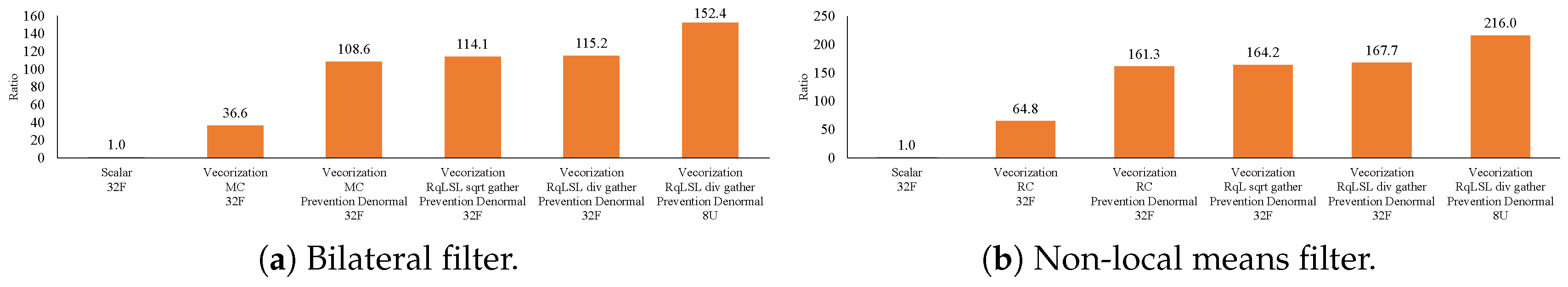
• MC: merged computing; range and spatial kernels are merged and directly computed.
• RCSL: range computing spatial LUT; the range kernel is directly computed, and LUTs are used for the spatial kernel.
• RLSC: range LUT spatial computing; LUTs are used for the range kernel, and the spatial kernel is directly computed.
• RLSL: range LUT spatial LUT; LUTs are used for both range and spatial kernels.
• ML: merged LUT; LUTs are used for the merged range and spatial kernels;
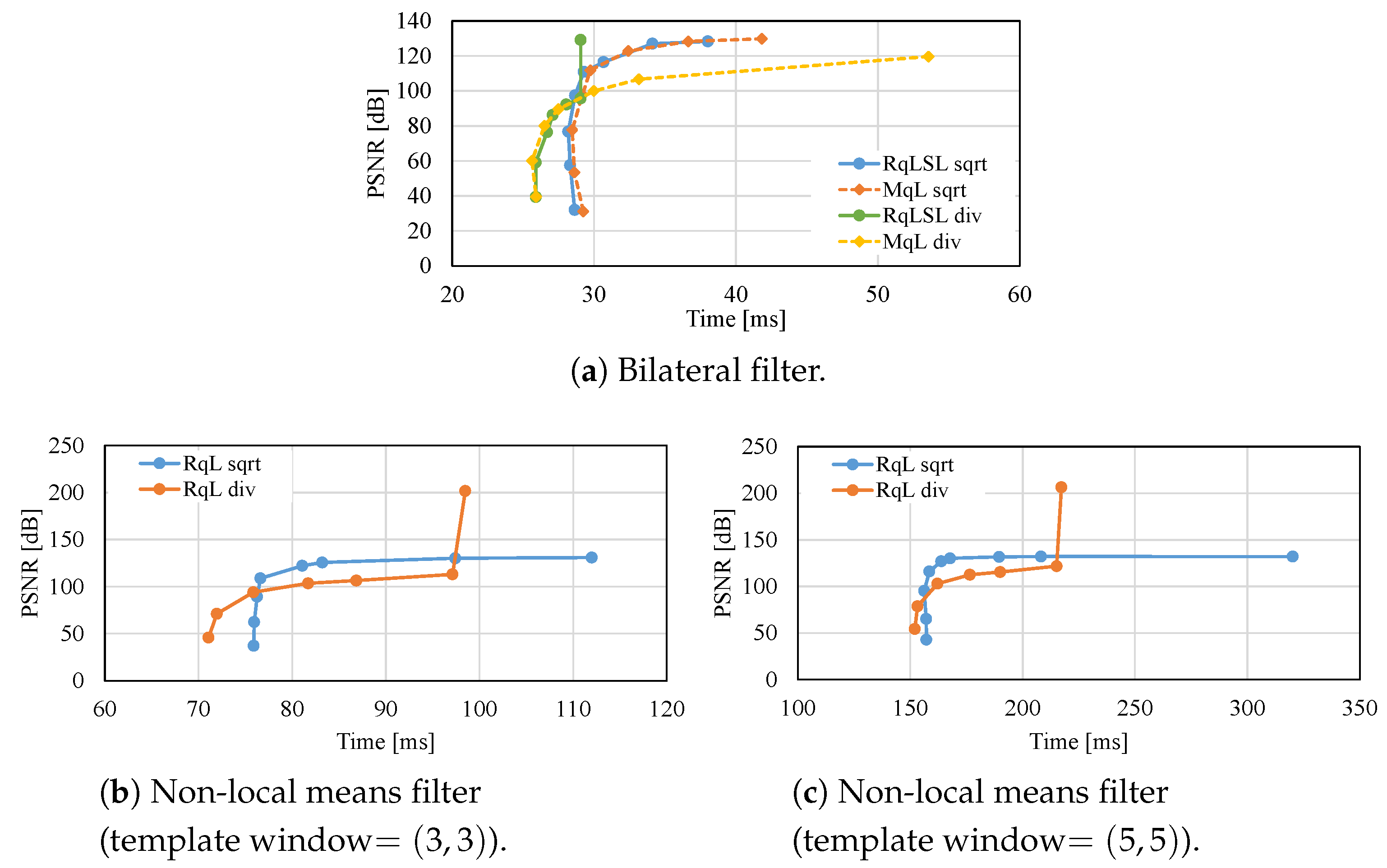
• RqLSL, RLSqL: range (quantized) LUT spatial (quantized) LUT; LUTs are quantized for each range and spatial LUT in RLSL
• MqL: merged quantized LUT; range and spatial kernels are merged, and then, the LUTs are quantized.

In the non-local means filtering process, the possible types of implementation are reduced, because the filter does not contain the spatial kernel. The possible types of implementation are as follows:

• RC: range computing; the range kernel is directly computed.
• RL: range LUT; LUTs are used for the range kernel.
• RqL: range quantized LUT; quantized LUTs are used for the range kernel.

We consider five types of implementation for bilateral filtering, namely, MC, RCSL, RLSL, RqLSL and MqL. Notably, we did not implement the RCSC, RLSC, RLSqL and ML, because the cost of computing the spatial kernel is lower than that of computing the range kernel, and the size of the range/merged LUT is larger than that of the spatial LUT. We also implement three types for non-local means filtering, such as RC, RL and RqL. Note that the pairs of MC/RC, RLSL/RL and RqLSL/RqL are similar without spatial computation.

In the MC/RC implementation, weights are directly computed for each iteration. In the bilateral and bilateral non-local means filtering, two exponential terms are computed as one exponential term considering the nature of the exponential function. The implementation is computationally expensive because it involves weight calculation every time. However, this point is not always a drawback. The calculation increases arithmetic intensity, which is the ratio of the number of float-number operations per the amount of the accessed memory data. When the arithmetic intensity is low, the computational time is limited by memory reading/writing [48]. In image processing, arithmetic intensity tends to be low, but the MC/RC implementation improves the arithmetic intensity. Therefore, the MC/RC implementation may be practical in a few cases.

RCSL can be applied to filters, which contain a spatial kernel. These filters include the bilateral and bilateral non-local means filters. The exponential term of the range kernel is computed every time, and LUTs are used as the weights of the spatial kernel. The size of the spatial LUT is the kernel size. In the bilateral filters, the weight function in the proposed implementation can be expressed as follows:

$$\begin{array}{ccc}\hfill f(\mathit{p},\mathit{q})& :=& EX{P}_s[\mathit{p}-\mathit{q}]\exp (-\frac{{\parallel \mathit{I}(\mathit{p})-\mathit{I}(\mathit{q})\parallel }_2^2}{2{\sigma }_r^2}),\hfill \end{array}$$

(20)

$$\begin{array}{ccc}\hfill EX{P}_s[\mathit{x}]& :=& \exp (\frac{{\parallel \mathit{x}\parallel }_2^2}{-2{\sigma }_s^2}),\hfill \end{array}$$

(21)

where $EX{P}_s[·]$ is the spatial LUT. The first term is calculated for all possible arguments; subsequently, the weight values are stored in a LUT before filtering. Because the combinations of the relative distances of $\mathit{p}$ and $\mathit{q}$ are identical in all kernels, it is not required to calculate the relative distances for each kernel.

In RLSL/RL, LUTs are used as the weights of the range and the spatial kernels. The LUTs are created for the range or spatial kernel. For Gaussian range and non-local means filtering, the spatial kernel is omitted or always considered to be one. Only one LUT is used for the kernel, but the LUT is referenced for each channel using the separate representation of an exponential function. Notably, we can save the LUT size, which is 256. If we use an LUT for merged representation of an exponential function, its size becomes ${255}^2\times 3+1=$ 195,075. In the bilateral filter for a color image, the weight function of the implementation is expressed as follows:

$$\begin{array}{ccc}\hfill f(\mathit{p},\mathit{q})& :=& EX{P}_s[\mathit{p}-\mathit{q}]\hfill \\ & & EX{P}_r{[\lfloor \parallel \mathit{I}(\mathit{p})}_r-\mathit{I}{(\mathit{q})}_r{\parallel }_1\rfloor ]EX{P}_r{[\lfloor \parallel \mathit{I}(\mathit{p})}_g-\mathit{I}{(\mathit{q})}_g{\parallel }_1\rfloor ]EX{P}_r{[\lfloor \parallel \mathit{I}(\mathit{p})}_b-\mathit{I}{(\mathit{q})}_b{\parallel }_1\rfloor ]\hfill \end{array}$$

(22)

$$\begin{array}{ccc}\hfill EX{P}_r[x]& :=& \exp (\frac{x^2}{-2{\sigma }_r^2}),\hfill \end{array}$$

(23)

where $\lfloor ·\rfloor$ is the floor function, ${\parallel ·\parallel }_1$ is the L1 norm and $\mathit{I}{(·)}_r$, $\mathit{I}{(·)}_g$ and $\mathit{I}{(·)}_b$ are the red, green and blue channels in $\mathit{I}(·)$, respectively. $EX{P}_r[·]$ is the range LUT, and $EX{P}_s[·]$ is identical to Equation (21). These LUTs are accessed frequently. Hence, the arithmetic intensity is low.

In RqLSL/RqL, the range LUT for the merged representation of an exponential function is quantized to reduce the LUT size. Therefore, the LUT is approximated. This implementation is faster than using a large LUT and accessing the LUT multiple times, such as RLSL/RL. In the bilateral filter, the weight function of the implementation is expressed as follows:

$$\begin{array}{ccc}\hfill f(\mathit{p},\mathit{q})& :=& EX{P}_s[\mathit{p}-\mathit{q}]EX{P}_{rq}{[\lfloor \varphi (\parallel \mathit{I}(\mathit{p})-\mathit{I}(\mathit{q})\parallel }_2^2)\rfloor ],\hfill \end{array}$$

(24)

$$\begin{array}{ccc}\hfill EX{P}_{rq}[x]& :=& \exp (\frac{\psi (x)}{-2{\sigma }_r^2}),\hfill \end{array}$$

(25)

where $\varphi (·)$ and $\psi (·)$ denote a quantization function and an inverse quantization function, respectively. By converting the range of the argument through the quantization function, the size of the LUT can be reduced. The LUT size is $\lfloor \varphi (3\times {255}^2)\rfloor +1$. We use the square root function (sqrt) and division for the quantization function. In sqrt, the quantization function and the inverse quantization function are expressed as follows:

$$\begin{array}{ccc}\hfill \varphi (x)& :=& n\sqrt{x},\hfill \end{array}$$

(26)

$$\begin{array}{ccc}\hfill \psi (x)& :=& \frac{x^2}{n^2},\hfill \end{array}$$

(27)

where n controls the LUT size. In div, they are expressed as follows:

$$\begin{array}{ccc}\hfill \varphi (x)& :=& \frac{x}{n},\hfill \end{array}$$

(28)

$$\begin{array}{ccc}\hfill \psi (x)& :=& x\times n.\hfill \end{array}$$

(29)

In sqrt, the size of the quantization range LUT is $442=\lfloor \sqrt{3\times {255}^2}\rfloor +1$. In div, it is 195,076 $=3\times {255}^2+1$, where $n=1$.

In MqL, the range and spatial LUTs are merged, and then, the LUT is quantized. This implementation uses only one LUT. Thus, we do not require to multiply the range and spatial kernels. In the MqL, the weight function of the bilateral filter is expressed as follows:

$$\begin{array}{ccc}\hfill f(\mathit{p},\mathit{q})& :=& EX{P}_{rq}[\lfloor \varphi (\frac{{\sigma }_r^2}{{\sigma }_s^2}{\parallel \mathit{p}-\mathit{q}\parallel }_2^2{+\parallel \mathit{I}(\mathit{p})-\mathit{I}(\mathit{q})\parallel }_2^2)\rfloor ],\hfill \end{array}$$

(30)

where $EX{P}_{rq}[·]$ is identical to Equation (25). The other filters are implemented in the same way. The size of the quantization merged LUT is larger than that of the quantization range LUT. The quantization merged LUT can be accessed only once in the weight calculation. The accuracy decreases, as does the quantization range LUT.

Furthermore, we consider the data type of an input image. The typical data type of input images is unsigned char, although floating point numbers are used in filter processing. Therefore, unsigned char values of the input image are converted to float/double before the filtering or during the filtering. Note that float is typically used. The bit length of the double is longer than that of float. Hence, the computational time when using double is slower than that when using float. When the input type is unsigned char, we must convert pixel values redundantly to floating point numbers for every loaded pixel. The converting time is $SK$, where S and K are the image and kernel size, respectively. By contrast, if the input type is a floating point number, which is pre-converted before filtering, the conversion process can be omitted in filtering. The converting times is S. However, in the case of inputting unsigned char, the arithmetic intensity is higher than that of float. This is because the bit length of unsigned char is shorter than that of float. We should consider the tradeoff between the number of converting times and arithmetic intensity owing to the size of the image and kernel.

In the use of LUTs, these implementation approaches can be applied to arbitrary weight functions, which are not limited to the weighting functions consisting of exponential functions in the present study. Especially, if a weight function is computationally expensive, the use of a LUT is more practical.

Notably, in these types of implementations, the weight of the target pixels, which is at the center of the kernel, need not be calculated. The weight of the target pixels is always one. When r is small, this approach accelerates the filtering process somewhat.

7. Experimental Results

We verified the occurrence of denormalized numbers in the bilateral filtering, non-local means filtering, Gaussian range filtering and bilateral non-local means filtering processes. Moreover, we discussed the effective vectorization of bilateral filtering and non-local means filtering on the latest CPU microarchitectures. These filters were implemented in C++ by using OpenCV [49]. Additionally, multi-core parallelization was executed using Concurrency (https://msdn.microsoft.com/en-us/library/dd492418.aspx), which is a parallelization library provided by Microsoft, also called the parallel patterns library (PPL).

Table 2. Computers used in the experiments.

CPU	Intel Core i7 3970X	Intel Core i7 4960X	Intel Core i7 5960X	Intel Core i7 6950X	Intel Core i9 7980XE	AMD Ryzen Threadripper 1920X
memory	DDR3-1600 6 GBytes	DDR3-1866 16 GBytes	DDR4-2133 32 GBytes	DDR4-2400 32 GBytes	DDR4-2400 16 GBytes	DDR4-2400 16 GBytes
SIMD instruction sets	SSE4.2 AVX	SSE4.2 AVX	SSE4.2 AVX/AVX2 FMA3	SSE4.2 AVX/AVX2 FMA3	SSE4.2 AVX/AVX2 AVX512F FMA3	SSE4.2 AVX/AVX2 FMA3

shows the CPUs, SIMD instruction sets and memory employed in our experiments. Windows 10 64-bit was used as the OS, and Intel Compiler 18.0 was employed. For referring LUTs, the set or gather SIMD instructions were employed. The outermost loop was parallelized by multi-core threading, and we had pixel-loop vectorization [50]. This implementation was found to be the most effective [50]. Notably, a vectorized exponential operation is not implemented in these CPUs. Hence, we employed a software implementation, which is available in Intel Compiler. The experimental code spanned around 95,000 lines (https://github.com/yoshihiromaed/FastImplementation-BilateralFilter).

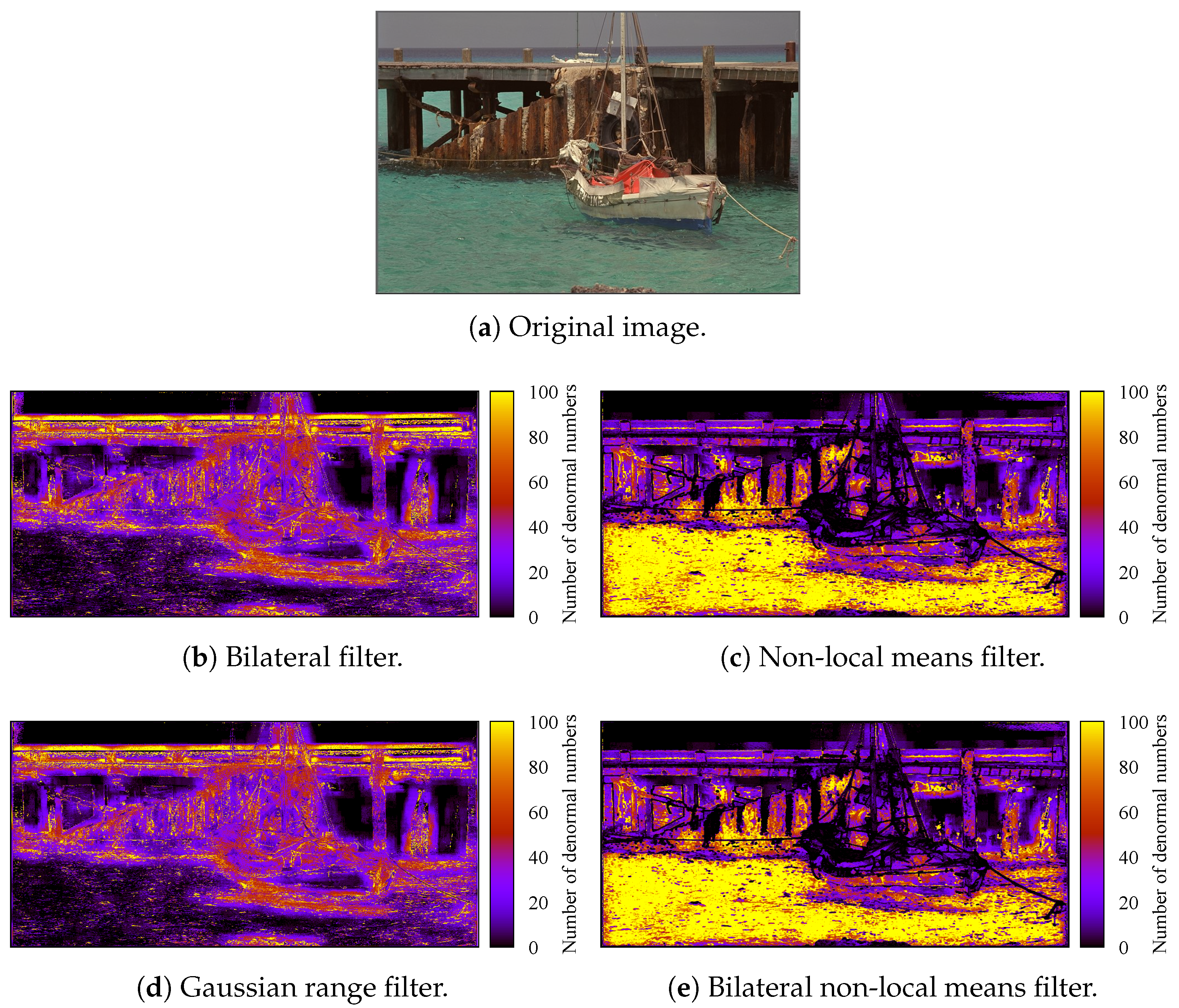
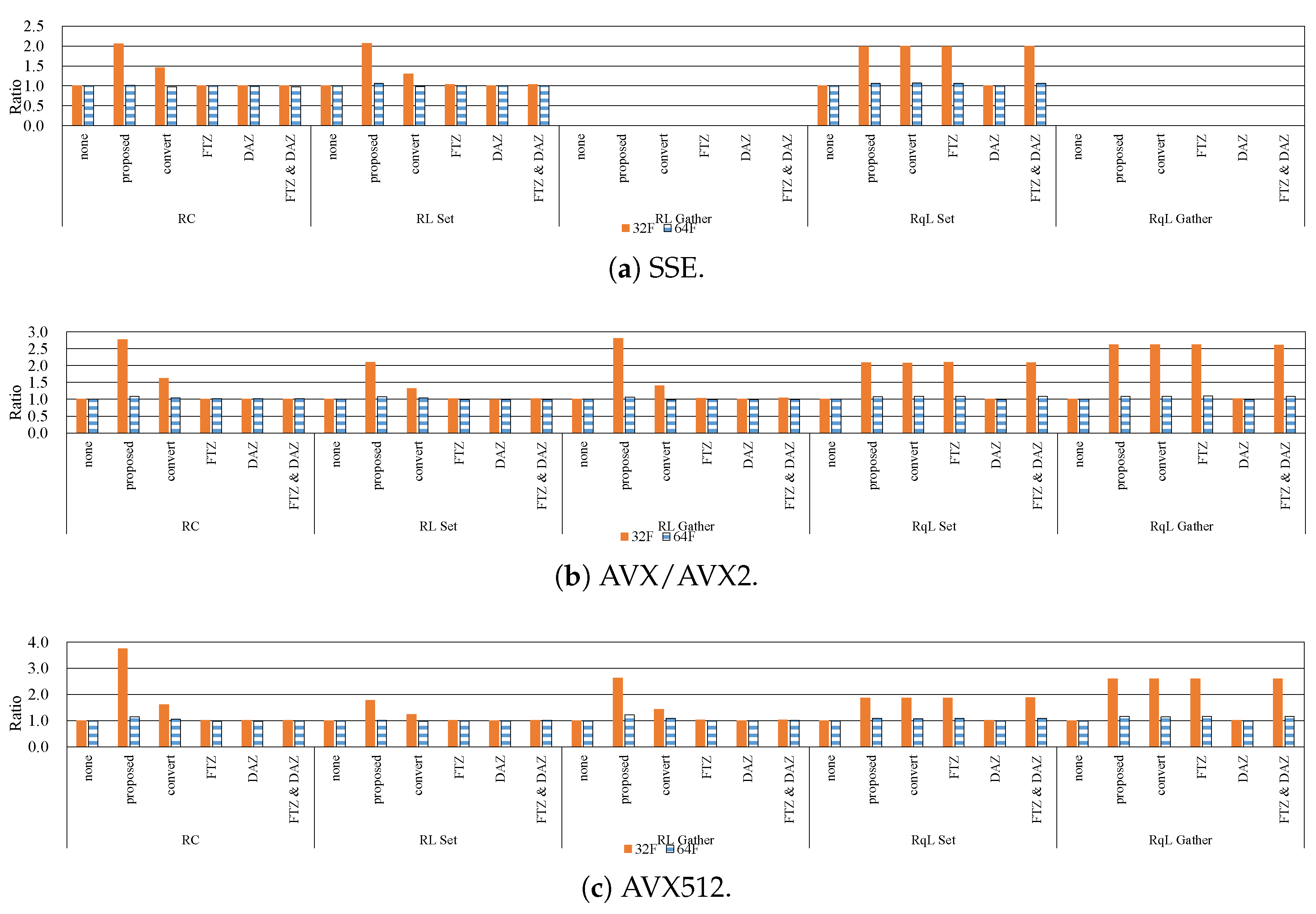
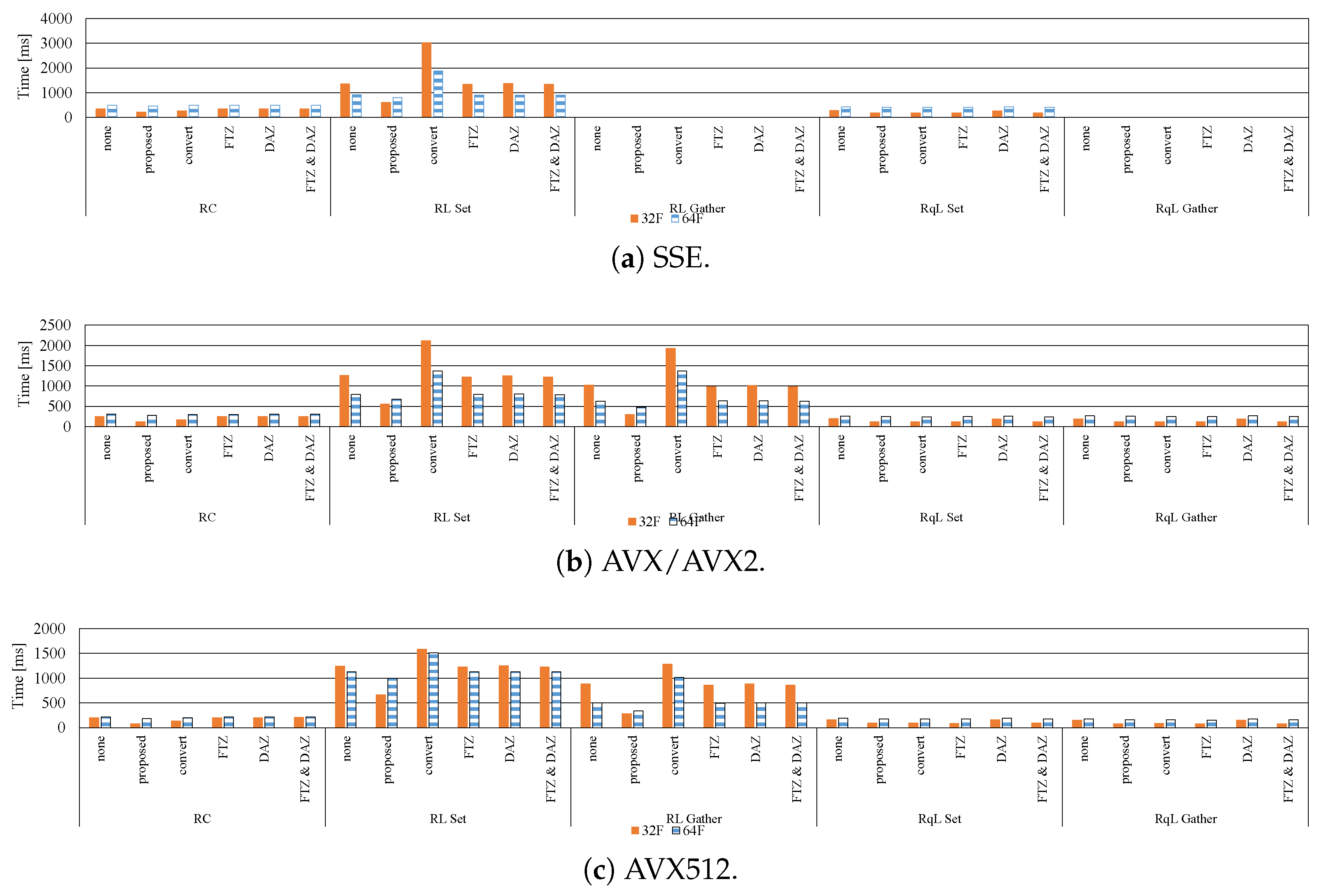
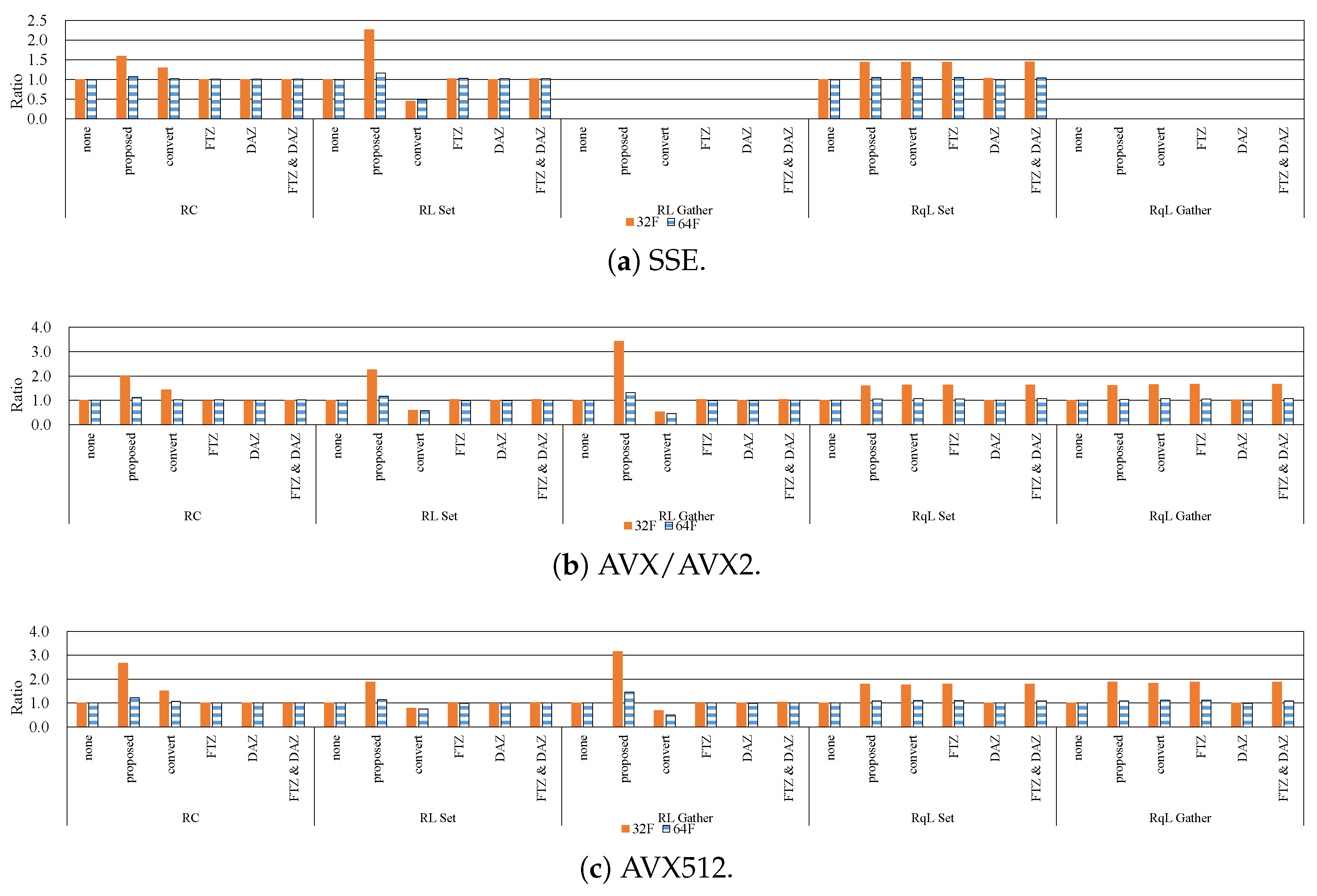
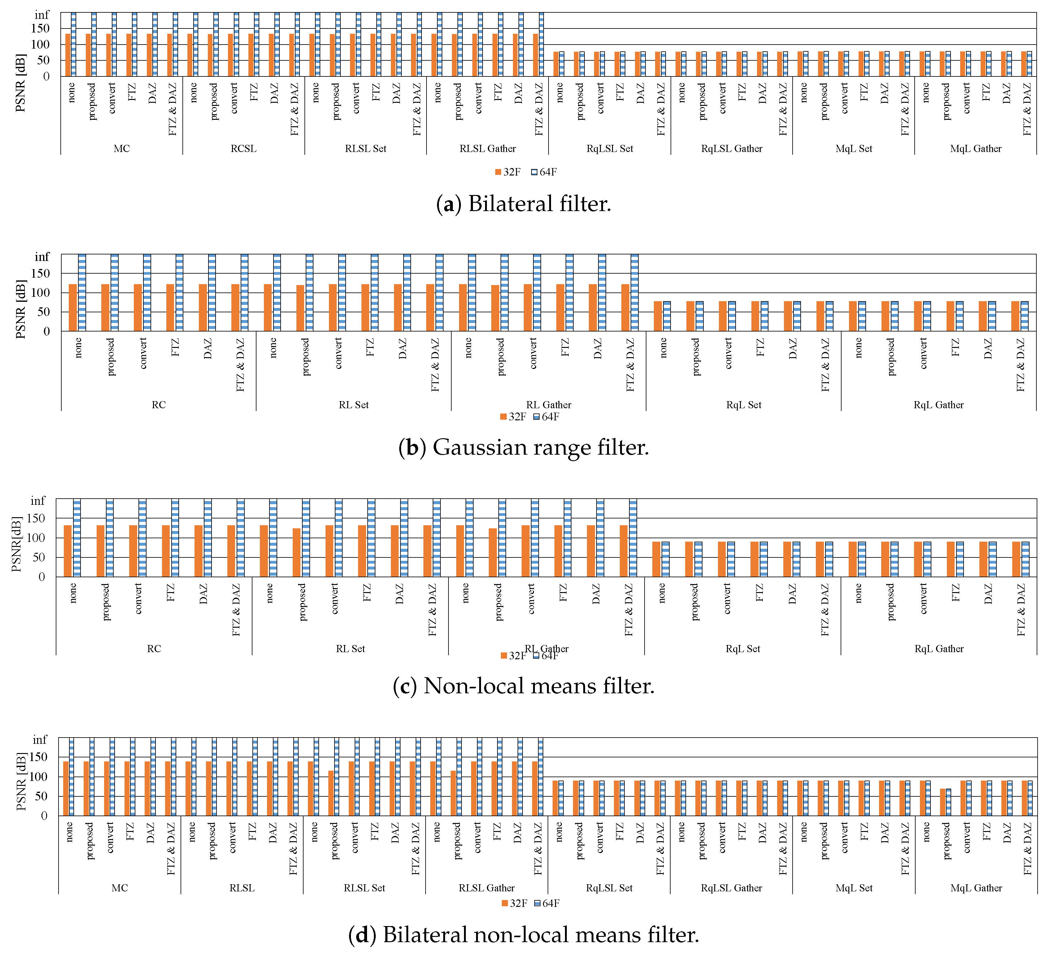
7.1. Influence of Denormalized Numbers

We compared the proposed methods with the straightforward approach (none) and four counter-approaches for denormalized numbers. These approaches involve converting denormalized numbers to normal numbers (convert) and using FTZ and/or DAZ flags (FTZ, DAZ, and FTZ and DAZ). The convert implementation clips a calculated value to a normal number value in the weight calculation by means of a min-operation with the minimal value of the normal numbers, such as $\min (exp(a)\times exp(b),v)$, where a and b are variables and v is the minimal value of the normal numbers. Figure 3, Figure 4, Figure 5, Figure 6, Figure 7, Figure 8, Figure 9 and Figure 10 show the results of computational time and speedup ratio of various types of implementation on Intel Core i9 7980XE. The computational time was taken as the median value of 100 trials. The parameters were identical for all filters. Notably, in the RqLSL/RqL and MqL implementation, sqrt was used as the quantization function, and $n=1$. These figures indicate that the proposed methods for handing denormalized number were the fastest among the other approaches for each implementation. The proposed methods were up to four-times faster than the straightforward approach. In many cases, the none implementation using double was faster than that using float. The range of magnitudes of double was larger than that of float. Hence, the occurrence frequency of denormalized numbers was lower. In the case of double, however, there was no significant speedup in all approaches for managing denormalized numbers. Because double had twice the byte length compared to float, the corresponding computational time was approximately twice as long, as well. Therefore, the implementation using double was slower than that using float when the influence of denormalized numbers was eliminated. In the RqL of the Gaussian range and the non-local means filters and the MqL of the bilateral and bilateral non-local means filters, the speedup ratio of the proposed methods was almost the same as that of the convert, FTZ and FTZ and DAZ implementation. In these approaches, denormalized numbers occurred only when LUTs were created, and the denormalized numbers were eliminated during LUT creation. Thus, during the filtering process, denormalized numbers did not occur. Therefore, the RqL and MqL implementation could achieve the same effect as the proposed methods did. In addition, DAZ had almost no effect because DAZ was executed only if an operand was a denormalized number. As shown in Figure 1, denormalized numbers occurred in edges. Therefore, if the weight of the range kernel was small or the multiplication of the range kernel with the spatial kernel was possible, denormalized numbers were likely to occur.

Table 3. Computational time and speedup ratio of bilateral filtering in the merged computing (MC) implementation using AVX512 for various parameters. These results were obtained on an Intel Core i9 7980XE. If the ratio exceeds 1, the proposed methods are faster than the straightforward implementation (none) for each parameter. $r=3{\sigma }_s$, and image size is 768 × 512. (a) Computational time (proposed) [ms]; (b) Computational time (none) [ms]; (c) Speedup ratio.

(a)						(b)						(c)
	σr	4	8	16			σr	4	8	16			σr	4	8	16
σs						σs						σs
4		17.48	17.57	17.63		4		66.48	51.36	50.24		4		3.80	2.92	2.85
8		43.96	43.86	43.73		8		217.55	194.94	192.96		8		4.95	4.45	4.41
16		147.76	147.58	147.50		16		763.87	755.56	719.00		16		5.17	5.12	4.87

,

Table 4. Computational time and speedup ratio of Gaussian range filter in the range computing (RC) implementation using AVX512 for various parameters. These results were obtained on an Intel Core i9 7980XE. If the ratio exceeds 1, the proposed methods are faster than the straightforward implementation (none) for each parameter. Image size is 768 × 512. (a) Computational time (proposed) [ms]; (b) Computational time (none) [ms]; (c) Speedup ratio.

(a)						(b)						(c)
	σr	4	8	16			σr	4	8	16			σr	4	8	16
r						r						r
12		16.76	16.83	16.85		12		63.95	48.69	48.09		12		3.82	2.89	2.85
24		42.53	42.40	42.39		24		207.54	185.16	181.40		24		4.88	4.37	4.28
48		143.24	143.01	142.58		48		741.42	717.41	685.18		48		5.18	5.02	4.81

,

Table 5. Computational time and speedup ratio of non-local means filter in the RC implementation using AVX512 for various parameters. These results were obtained on an Intel Core i9 7980XE. If the ratio exceeds 1, the proposed methods are faster than the straightforward implementation (none) for each parameter. Template window size is $(3,3)$, and image size is 768 × 512. (a) Computational time (proposed) [ms]; (b) Computational time (none) [ms]; (c) Speedup ratio.

(a)						(b)						(c)
	h	4$\sqrt{2}$	8$\sqrt{2}$	16$\sqrt{2}$			h	4$\sqrt{2}$	8$\sqrt{2}$	16$\sqrt{2}$			h	4$\sqrt{2}$	8$\sqrt{2}$	16$\sqrt{2}$
Search Window						Search Window						Search Window
(25, 25)		40.31	39.80	39.64		(25, 25)		98.91	82.84	80.66		(25, 25)		2.45	2.08	2.03
(49, 49)		128.90	128.90	128.90		(49, 49)		332.88	307.58	300.00		(49, 49)		2.58	2.39	2.33
(97, 97)		485.88	485.88	485.36		(97, 97)		1148.48	1158.53	1134.93		(97, 97)		2.36	2.38	2.34

and

Table 6. Computational time and speedup ratio of the bilateral non-local means filter in the MC implementation using AVX512 for various parameters. These results were calculated using an Intel Core i9 7980XE. If the ratio exceeds 1, the proposed methods are faster than the straightforward implementation (none) for each parameter. Template window size is $(3,3)$; search window size is $(2\times 3{\sigma }_s+1,2\times 3{\sigma }_s+1)$; and image size is 768 × 512. (a) Computational time (proposed) [ms]; (b) Computational time (none) [ms]; (c) Speedup ratio.

(a)						(b)						(c)
	h	4$\sqrt{2}$	8$\sqrt{2}$	16$\sqrt{2}$			h	4$\sqrt{2}$	8$\sqrt{2}$	16$\sqrt{2}$			h	4$\sqrt{2}$	8$\sqrt{2}$	16$\sqrt{2}$
σs						σs						σs
4		40.20	40.05	39.92		4		99.14	84.85	82.85		4		2.47	2.12	2.08
8		133.61	133.02	132.85		8		340.29	311.72	301.38		8		2.55	2.34	2.27
16		496.86	496.57	495.89		16		1166.17	1191.36	1163.34		16		2.35	2.40	2.35

show the speedup ratio of the MC/RC implementation between the proposed methods and the none implementation for each set of smoothing parameters. Note that when ${\sigma }_s$, r, and the search window size are larger, the amount of processing increases. The tables indicate that the proposed methods are 2–5-times faster than the none implementation. When the smoothing parameters are small and the amount of processing is large, the speedup ratio is high. Therefore, the influence of denormalized numbers is strong when the degree of smoothing is small and the amount of processing is large.

To verify the accuracy of the proposed methods, we compared the scalar implementation in double-precision with the proposed methods and other approaches regarding peak signal-to-noise ratio (PSNR). The results are shown in Figure 11. The proposed methods hardly affect accuracy. Note that the accuracies of the RqL and MqL implementation are slightly lower than those of the other types of implementation because the LUTs are approximated. In these types, the accuracy deterioration is not significant because human vision does not sense differences higher than 50 dB [51,52].

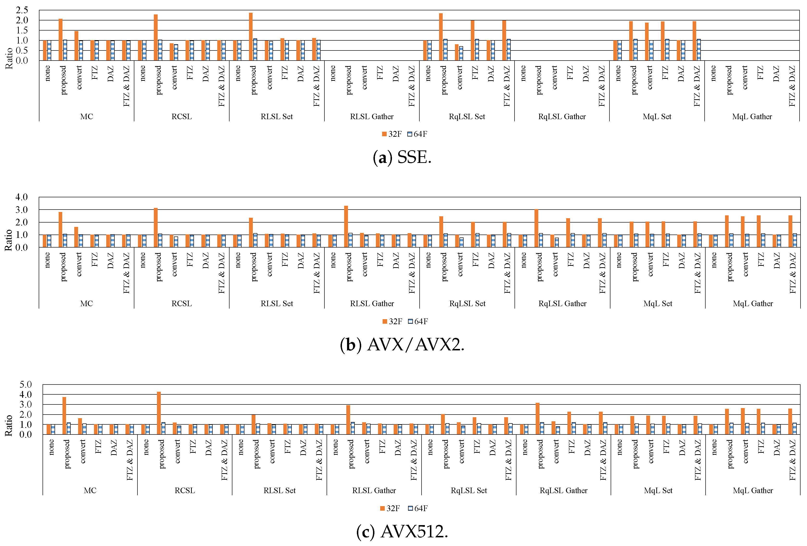
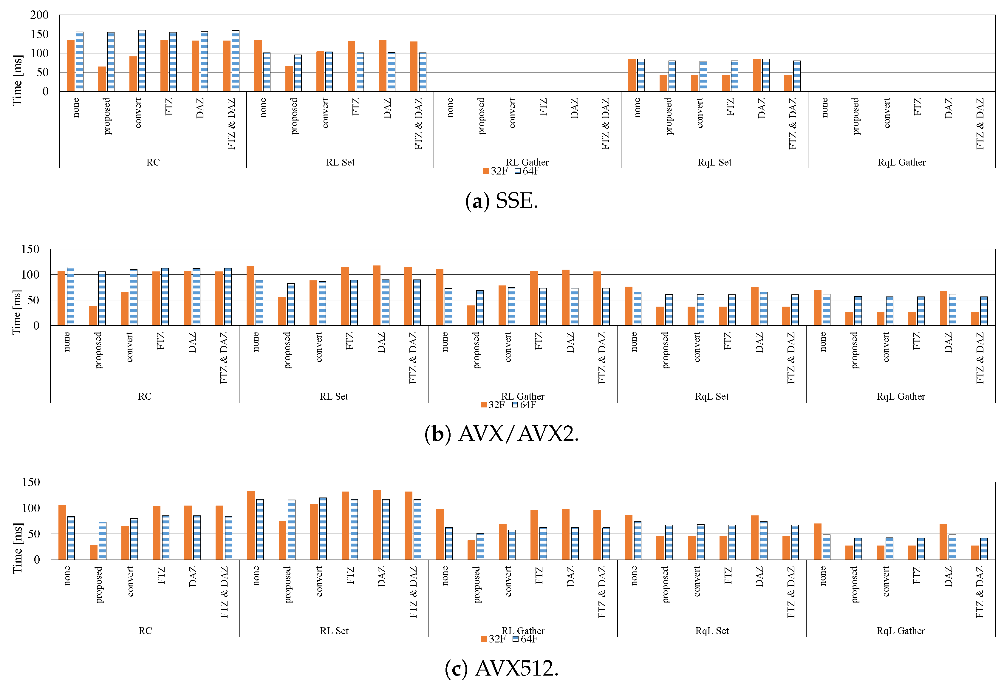
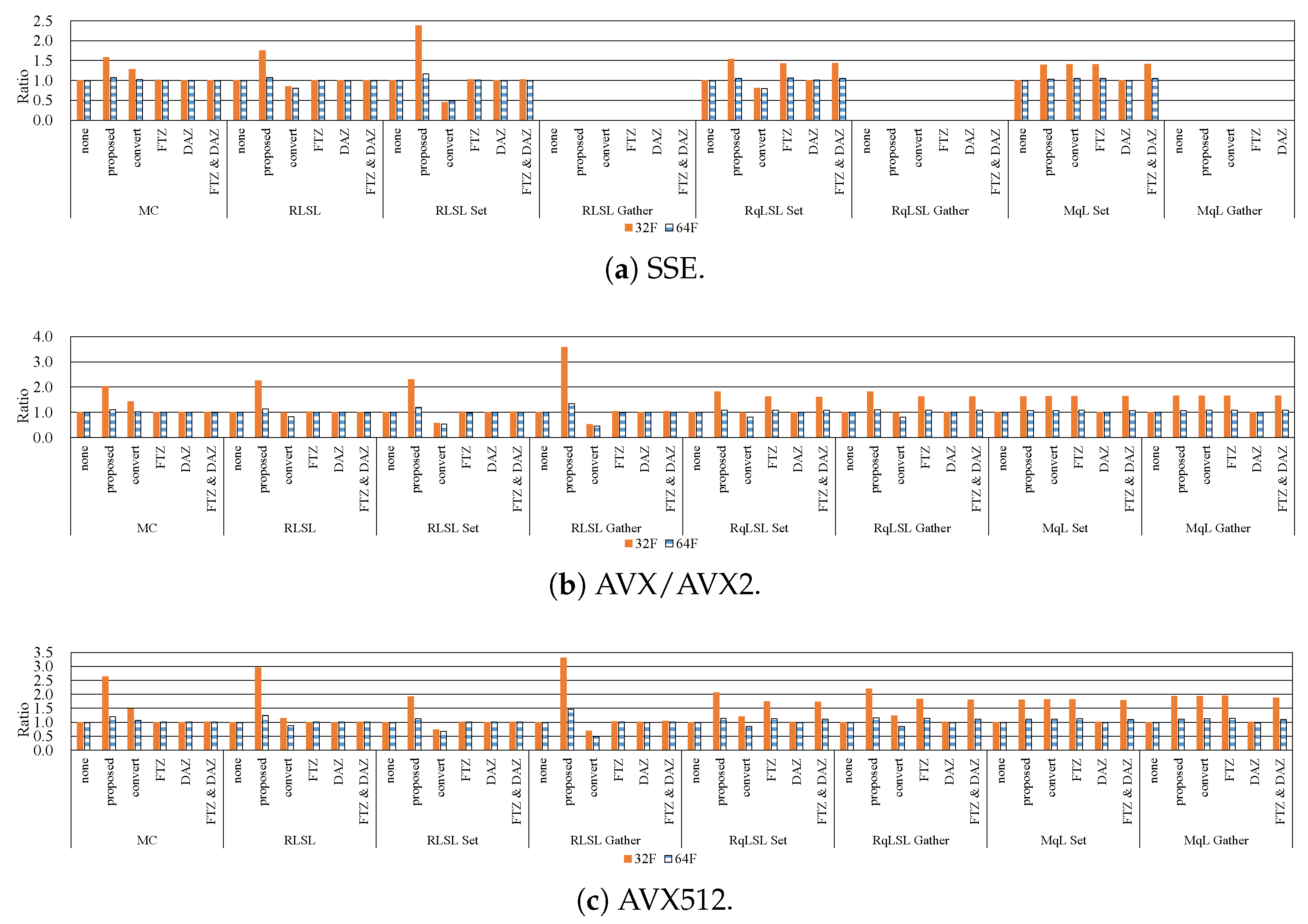
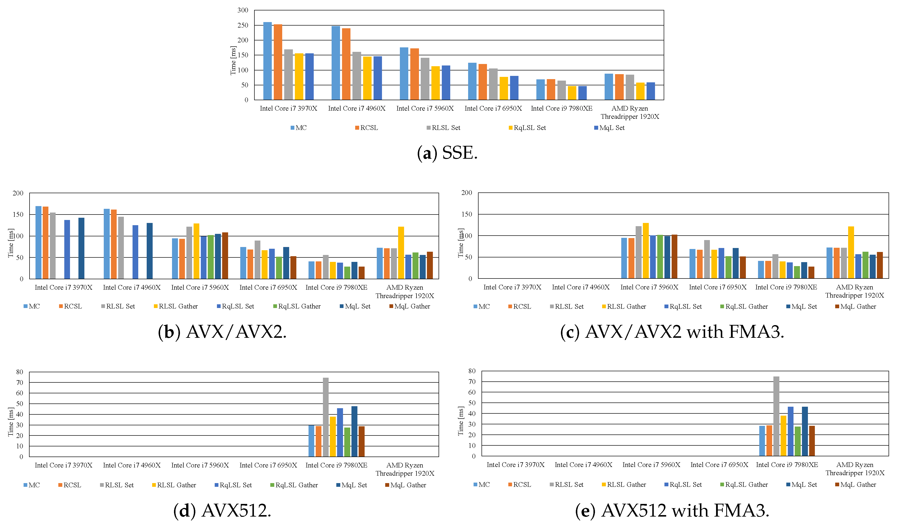
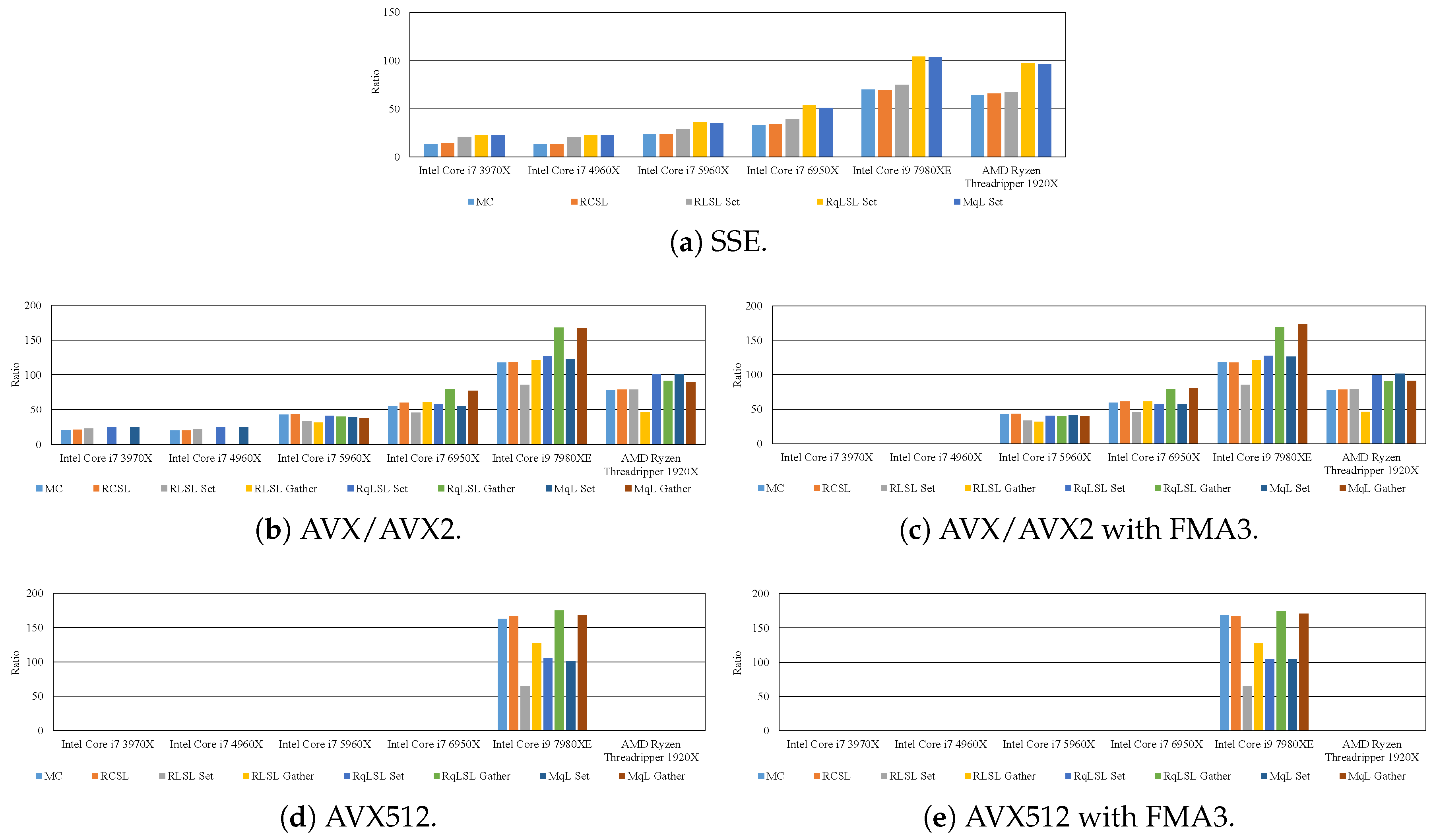
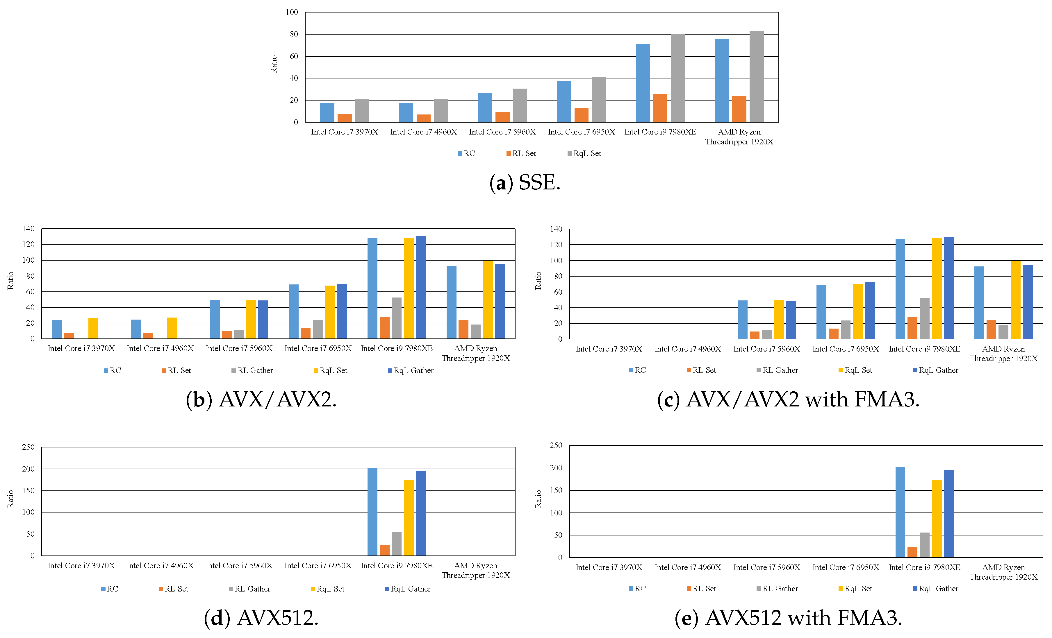
7.2. Effective Implementation on CPU Microarchitectures

In this subsection, we verify the effective vectorization of the bilateral filter and the non-local means filter on the latest CPU microarchitectures. The proposed methods for denormalized numbers have already been applied to these filters. Figure 12 and Figure 13 show the computational times of the bilateral filter and the non-local means filter for each CPU microarchitecture. These filters were implemented using float. Notably, in the RqLSL/RqL and MqL implementation, sqrt was used as the quantization function and $n=1$. The RqLSL/RqL implementation is the fastest in these CPU microarchitectures. This implementation has a lower computational cost than the MC/RC implementation. Moreover, the number of LUT accesses is lower than that in the case of the RLSL/RL implementation. The computational time of the MC/RC implementation is almost the same as that of the RLSL/RL and RqLSL/RqL implementation or faster than that of the RLSL/RL implementation. This tendency can be stronger in the latest CPU microarchitectures because computational time is limited by the memory reading/writing latency. Besides, the computation time of the RqLSL implementation is almost the same as that of the MqL implementation, but that of the RqLSL implementation is slightly faster than that of the MqL implementation. The size of the merged quantization LUT is larger than that of the range quantization LUT. The effects of the size of the quantization LUT and the quantization function are discussed in the following paragraph. The RLSL/RL, RqLSL/RqL and MqL implementations in which the gather instruction is employed are faster than the implementations in which the set instruction is employed. However, on the Intel Core i7 5960X and AMD Ryzen Threadripper 1920X CPUs, the implementations in which the gather instruction is used are slower than the implementations in which the set instruction is used. In the bilateral filter and the non-local means filter, when the SIMD’s vector length increases, all types of implementations with longer SIMD instructions are faster than that with shorter SIMD instructions. Furthermore, in a comparison of the implementations with/without FMA3, the FMA3 instruction improved computational performance slightly. These results indicate that effective vectorization of the bilateral filter and the non-local means filter are different for each CPU microarchitecture. Figure 14 and Figure 15 show the speedup ratio of the bilateral filter and the non-local means filter for each CPU microarchitecture. If the ratio exceeds one, the corresponding implementation is faster than the scalar implementation for each CPU microarchitecture. Multi-core threading parallelized both the scalar and the vectorized implementations for focusing on comparing vectorized performance. In the case of the bilateral filter, the fastest implementation is 170-times faster than the scalar one. Moreover, in the case of the non-local means filter, the fastest implementation is 200-times faster than the scalar one. The speedup was determined by the management of denormalized numbers and effective vectorization. Thus, the effect of using a multi-core CPU is not evaluated in the verification.

We discuss the relationship between accuracy and computational time for various types of implementation involving the use of the quantization LUT. Figure 16 shows the relationship between calculation time and accuracy of the RqL and the MqL implementation. In this figure, we changed the quantization functions and the size of the quantization range/merged LUTs. The quantization functions were square root function (sqrt) and division (div). Note that the maximal value in the case of the RqLSL/RqL implementation is commensurate with that of the non-quantized cases. In the RqLSL/RqL and MqL implementation, the accuracy and computational time have a trade-off. These implementations accelerate these filters while maintaining high accuracy, when the LUT size is practical. The characteristics of the performance depend on the quantization functions. Therefore, we must choose the functions and the LUT size by considering the required accuracy and computational time.

Figure 17 shows the computational time of using unsigned char (8U) and float (32F) in the MC/RC implementation. Note that the computational time is plotted on a logarithmic scale. The 8U implementation of the bilateral filter is faster than the 32F implementation, when r is small. By contrast, when r is large, the 8U implementation is slower than the 32F implementation. If the cost of the conversion process in 8U is low, the arithmetic intensity of the 8U implementation would be larger than that of the 32F implementation. However, in the 8U implementation, the conversion cost increases owing to the redundant conversion of the pixels as the amount of processing increases. In the non-local means filter, when the template window size is $(3,3)$, the 8U implementation is always faster than the 32F implementation. When the template window size is $(5,5)$, the 8U implementation is slower than the 32F implementation in the case of the large search window. The arithmetic intensity of the non-local means filter is low because many pixels are accessed. Therefore, we can improve the arithmetic intensity by using the 8U implementation. However, if the amount of processing is large, we should use 32F. As a result, the speeds of the 8U and 32F implementation depend on the amount of processing, which are changed by the filtering kernel size and arithmetic intensity.

Figure 18 shows the speedup ratio of each implementation of the proposed methods for prevention of denormalized numbers. If the speedup ratio exceeds one, the implementation is faster than the scalar implementation. All types of implementation were parallelized by multi-core threading. The figure shows that the fastest implementation of the bilateral filter and the non-local means filter is 152- and 216-times faster than the scalar implementation, respectively. Therefore, we can achieve significant acceleration by applying the proposed methods for preventing the occurrence of denormalized numbers and selecting the implementation approaches of weight calculation and the appropriate data type.

Finally, we compared the fastest implementation with OpenCV, which is the de facto standard image processing library [49]. Figure 19 shows the computational times of our implementation and the OpenCV’s implementation with its speedup ratio. Notably, the computational time is plotted on the logarithmic scale. Our method is 2–14-times faster than OpenCV. In the OpenCV implementation, the distance function of the range kernel is not the L2 norm, and the kernel shape is circular for acceleration (see Appendix A); therefore, PSNR is low. By contrast, our implementation slightly approximates the kernel LUT, and the kernel shape is rectangular. Therefore, the proposed methods are more practical.

8. Conclusions

In this paper, we propose methods to accelerate bilateral filtering and non-local means filtering. The proposed methods prevent the occurrence of denormalized numbers, which has a large computational cost for processing. Moreover, we verify various types of vectorized implementations on the latest CPU microarchitectures. The results are summarized as follows:

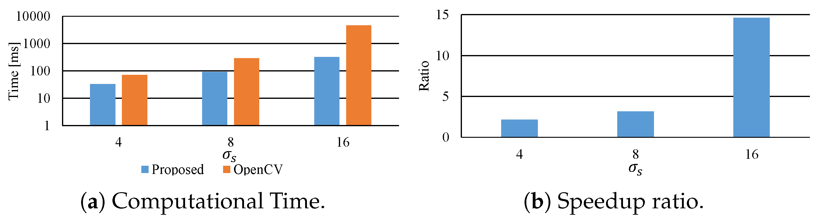
• The proposed methods are up to five-times faster than the implementation without preventing the occurrence of denormalized numbers.
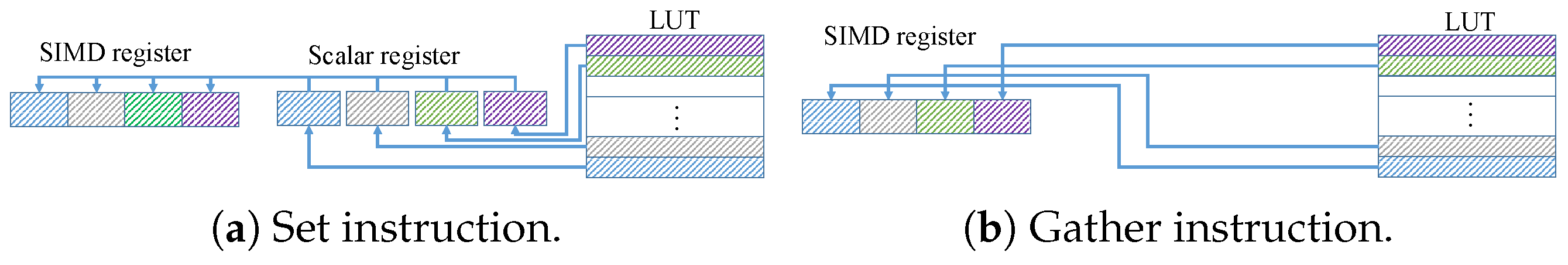
• In modern CPU microarchitectures, the gather instruction in the SIMD instruction set is effective for loading weights from the LUTs.
• By reducing the LUT size through quantization, the filtering can be accelerated while maintaining high accuracy. Moreover, the optimum quantization function and the quantization LUT size depends on the required accuracy and computational time.
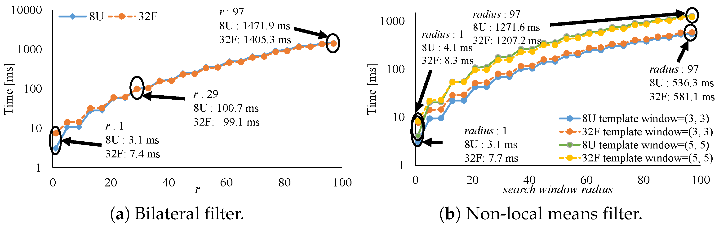
• When the kernel size is small, the 8U implementation is faster than the 32F implementation. By contrast, in the case of the large kernel, the 32F implementation is faster than the 8U implementation.

In the future, we will verify the influence of denormalized numbers on GPUs. In particular, we are planning to implement edge-preserving filters on GPUs and to verify the influence of the denormalized numbers on computation time in GPUs. Furthermore, we will design effective implementations of the filters on GPUs.

References

1. Tomasi, C.; Manduchi, R. Bilateral Filtering for Gray and Color Images. In Proceedings of the IEEE International Conference on Computer Vision (ICCV), Bombay, India, 4–7 January 1998; pp. 839–846. [Google Scholar]
2. Paris, S.; Kornprobst, P.; Tumblin, J.; Durand, F. Bilateral Filtering: Theory and Applications; Now Publishers Inc.: Delft, The Netherlands, 2009. [Google Scholar]
3. Buades, A.; Coll, B.; Morel, J.M. A Non-Local Algorithm for Image Denoising. In Proceedings of the IEEE Conference on Computer Vision and Pattern Recognition (CVPR), San Diego, CA, USA, 20–25 June 2005; pp. 60–65. [Google Scholar]
4. He, K.; Sun, J.; Tang, X. Guided Image Filtering. IEEE Trans. Pattern Anal. Mach. Intell. 2013, 35, 1397–1409. [Google Scholar] [CrossRef] [PubMed]
5. He, K.; Sun, J.; Tang, X. Guided Image Filtering. In Proceedings of the European Conference on Computer Vision (ECCV), Crete, Greece, 5–11 Septembe 2010. [Google Scholar]
6. Fukushima, N.; Sugimoto, K.; Kamata, S. Guided Image Filtering with Arbitrary Window Function. In Proceedings of the IEEE International Conference on Acoustics, Speech and Signal Processing (ICASSP), Calgary, AB, Canada, 15–20 April 2018. [Google Scholar]
7. Kang, W.; Yu, S.; Seo, D.; Jeong, J.; Paik, J. Push-Broom-Type Very High-Resolution Satellite Sensor Data Correction Using Combined Wavelet-Fourier and Multiscale Non-Local Means Filtering. Sensors 2015, 15, 22826–22853. [Google Scholar] [CrossRef] [PubMed] [Green Version]
8. Durand, F.; Dorsey, J. Fast Bilateral Filtering for the Display of High-Dynamic-Range Images. ACM Trans. Graph. 2002, 21, 257–266. [Google Scholar] [CrossRef]
9. Bae, S.; Paris, S.; Durand, F. Two-Scale Tone Management for Photographic Look. ACM Trans. Graph. 2006, 25, 637–645. [Google Scholar] [CrossRef]
10. Fattal, R.; Agrawala, M.; Rusinkiewicz, S. Multiscale Shape and Detail Enhancement from Multi-Light Image Collections. ACM Trans. Graph. 2007, 26, 51. [Google Scholar] [CrossRef]
11. Li, L.; Si, Y.; Jia, Z. Remote Sensing Image Enhancement Based on Non-Local Means Filter in NSCT Domain. Algorithms 2017, 10, 116. [Google Scholar] [CrossRef]
12. Mori, Y.; Fukushima, N.; Yendo, T.; Fujii, T.; Tanimoto, M. View Generation with 3D Warping using Depth Information for FTV. Signal Process. Image Commun. 2009, 24, 65–72. [Google Scholar] [CrossRef]
13. Petschnigg, G.; Agrawala, M.; Hoppe, H.; Szeliski, R.; Cohen, M.; Toyama, K. Digital Photography with Flash and No-Flash Image Pairs. ACM Trans. Graph. 2004, 23, 664–672. [Google Scholar] [CrossRef]
14. Eisemann, E.; Durand, F. Flash Photography Enhancement via Intrinsic Relighting. ACM Trans. Graph. 2004, 23, 673–678. [Google Scholar] [CrossRef]
15. Kopf, J.; Cohen, M.; Lischinski, D.; Uyttendaele, M. Joint Bilateral Upsampling. ACM Trans. Graph. 2007, 26, 96. [Google Scholar] [CrossRef]
16. Zhou, D.; Wang, R.; Lu, J.; Zhang, Q. Depth Image Super Resolution Based on Edge-Guided Method. Appl. Sci. 2018, 8, 298. [Google Scholar] [CrossRef]
17. Kodera, N.; Fukushima, N.; Ishibashi, Y. Filter Based Alpha Matting for Depth Image Based Rendering. In Proceedings of the Visual Communications and Image Processing (VCIP), Kuching, Malaysia, 17–20 November 2013. [Google Scholar]
18. He, K.; Sun, J.; Tang, X. Single Image Haze Removal using Dark Channel Prior. In Proceedings of the Computer Vision and Pattern Recognition (CVPR), Miami, FL, USA, 20–24 June 2009. [Google Scholar]
19. Hosni, A.; Rhemann, C.; Bleyer, M.; Rother, C.; Gelautz, M. Fast Cost-Volume Filtering for Visual Correspondence and Beyond. IEEE Trans. Pattern Anal. Mach. Intell. 2013, 35, 504–511. [Google Scholar] [CrossRef] [PubMed]
20. Matsuo, T.; Fukushima, N.; Ishibashi, Y. Weighted Joint Bilateral Filter with Slope Depth Compensation Filter for Depth Map Refinement. In Proceedings of the International Conference on Computer Vision Theory and Applications (VISAPP), Barcelona, Spain, 21–24 February 2013; pp. 300–309. [Google Scholar]
21. Le, A.V.; Jung, S.W.; Won, C.S. Directional Joint Bilateral Filter for Depth Images. Sensors 2014, 14, 11362–11378. [Google Scholar] [CrossRef] [PubMed] [Green Version]
22. Liu, S.; Lai, P.; Tian, D.; Chen, C.W. New Depth Coding Techniques with Utilization of Corresponding Video. IEEE Trans. Broadcast. 2011, 57, 551–561. [Google Scholar] [CrossRef]
23. Fukushima, N.; Inoue, T.; Ishibashi, Y. Removing Depth Map Coding Distortion by Using Post Filter Set. In Proceedings of the International Conference on Multimedia and Expo (ICME), San Jose, CA, USA, 15–19 July 2013. [Google Scholar]
24. Fukushima, N.; Fujita, S.; Ishibashi, Y. Switching Dual Kernels for Separable Edge-Preserving Filtering. In Proceedings of the IEEE International Conference on Acoustics, Speech and Signal Processing (ICASSP), Brisbane, Australia, 19–24 April 2015. [Google Scholar]
25. Pham, T.Q.; Vliet, L.J.V. Separable Bilateral Filtering for Fast Video Preprocessing. In Proceedings of the International Conference on Multimedia and Expo (ICME), Amsterdam, The Netherlands, 6–9 July 2005. [Google Scholar]
26. Chen, J.; Paris, S.; Durand, F. Real-Time Edge-Aware Image Processing with the Bilateral Grid. ACM Trans. Graph. 2007, 26, 103. [Google Scholar] [CrossRef]
27. Sugimoto, K.; Fukushima, N.; Kamata, S. Fast Bilateral Filter for Multichannel Images via Soft-assignment Coding. In Proceedings of the APSIPA ASC, Jeju, Korea, 13–16 December 2016. [Google Scholar]
28. Sugimoto, K.; Kamata, S. Compressive Bilateral Filtering. IEEE Trans. Image Process. 2015, 24, 3357–3369. [Google Scholar] [CrossRef] [PubMed]
29. Paris, S.; Durand, F. A Fast Approximation of the Bilateral Filter using a Signal Processing Approach. Int. J. Comput. Vis. 2009, 81, 24–52. [Google Scholar] [CrossRef]
30. Chaudhury, K.N. Acceleration of the Shiftable O(1) Algorithm for Bilateral Filtering and Nonlocal Means. IEEE Trans. Image Process. 2013, 22, 1291–1300. [Google Scholar] [CrossRef] [PubMed]
31. Chaudhury, K. Constant-Time Filtering Using Shiftable Kernels. IEEE Signal Process. Lett. 2011, 18, 651–654. [Google Scholar] [CrossRef] [Green Version]
32. Chaudhury, K.; Sage, D.; Unser, M. Fast O(1) Bilateral Filtering Using Trigonometric Range Kernels. IEEE Trans. Image Process. 2011, 20, 3376–3382. [Google Scholar] [CrossRef] [PubMed]
33. Adams, A.; Gelfand, N.; Dolson, J.; Levoy, M. Gaussian KD-trees for fast high-dimensional filtering. ACM Trans. Graph. 2009, 28. [Google Scholar] [CrossRef]
34. Adams, A.; Baek, J.; Davis, M.A. Fast High-Dimensional Filtering Using the Permutohedral Lattice. Comput. Graph. Forum 2010, 29, 753–762. [Google Scholar] [CrossRef] [Green Version]
35. Porikli, F. Constant Time O(1) Bilateral Filtering. In Proceedings of the Computer Vision and Pattern Recognition (CVPR), Anchorage, AK, USA, 23–28 June 2008. [Google Scholar]
36. Yang, Q.; Tan, K.H.; Ahuja, N. Real-time O(1) bilateral filtering. In Proceedings of the Computer Vision and Pattern Recognition (CVPR), Miami, FL, USA, 20–24 June 2009; pp. 557–564. [Google Scholar]
37. IEEE. IEEE Standard for Floating-Point Arithmetic; IEEE Std 754-2008; IEEE: Piscataway, NJ, USA, 2008; pp. 1–70. [Google Scholar] [CrossRef]
38. Schwarz, E.M.; Schmookler, M.; Trong, S.D. FPU Implementations with Denormalized Numbers. IEEE Trans. Comput. 2005, 54, 825–836. [Google Scholar] [CrossRef]
39. Schwarz, E.M.; Schmookler, M.; Trong, S.D. Hardware Implementations of Denormalized Numbers. In Proceedings of the IEEE Symposium on Computer Arithmetic, Santiago de Compostela, Spain, 15–18 June 2003; pp. 70–78. [Google Scholar] [CrossRef]
40. Zheng, L.; Hu, H.; Yihe, S. Floating-Point Unit Processing Denormalized Numbers. In Proceedings of the International Conference on ASIC, Shanghai, China, 24–27 October 2005; Volume 1, pp. 6–9. [Google Scholar] [CrossRef]
41. Flynn, M.J. Some Computer Organizations and Their Effectiveness. IEEE Trans. Comput. 1972, 100, 948–960. [Google Scholar] [CrossRef]
42. Hughes, C.J. Single-Instruction Multiple-Data Execution. Synth. Lect. Comput. Archit. 2015, 10, 1–121. [Google Scholar] [CrossRef]
43. Kim, Y.S.; Lim, H.; Choi, O.; Lee, K.; Kim, J.D.K.; Kim, J. Separable Bilateral Nonlocal Means. In Proceedings of the International Conference on Image Processing (ICIP), Brussels, Belgium, 11–14 September 2011; pp. 1513–1516. [Google Scholar]
44. Moore, G.E. Cramming more components onto integrated circuits, Reprinted from Electronics, volume 38, number 8, April 19, 1965, pp.114 ff. IEEE Solid-State Circuits Soc. Newsl. 2006, 11, 33–35. [Google Scholar] [CrossRef]
45. Rotem, E.; Ginosar, R.; Mendelson, A.; Weiser, U.C. Power and thermal constraints of modern system-on-a-chip computer. In Proceedings of the International Workshop on Thermal Investigations of ICs and Systems (THERMINIC), Berlin, Germany, 25–27 September 2013; pp. 141–146. [Google Scholar] [CrossRef]
46. Intel Architecture Instruction Set Extensions and Future Features Programming Reference. Available online: https://software.intel.com/sites/default/files/managed/c5/15/architecture-instruction-set-extensions-programming-reference.pdf (accessed on 1 October 2018).
47. Ercegovac, M.D.; Lang, T. Digital Arithmetic, 1st ed.; Morgan Kaufmann Publishers Inc.: San Francisco, CA, USA, 2003. [Google Scholar]
48. Williams, S.; Waterman, A.; Patterson, D. Roofline: An Insightful Visual Performance Model for Multicore Architectures. Commun. ACM 2009, 52, 65–76. [Google Scholar] [CrossRef]
49. Bradski, G.; Kaehler, A. Learning OpenCV: Computer Vision with the OpenCV Library; O’Reilly Media, Inc.: Sevvan, CA, USA, 2008. [Google Scholar]
50. Maeda, Y.; Fukushima, N.; Matsuo, H. Taxonomy of Vectorization Patterns of Programming for FIR Image Filters Using Kernel Subsampling and New One. Appl. Sci. 2018, 8, 1235. [Google Scholar] [CrossRef]
51. Telegraph, I.; Committee, T.C. CCITT Recommendation T.81: Terminal Equipment and Protocols for Telematic Services: Information Technology–Digital Compression and Coding of Continuous-tone Still Images–Requirements and Guidelines; International Telecommunication Union: Geneva, Switzerland, 1993. [Google Scholar]
52. Domanski, M.; Rakowski, K. Near-Lossless Color Image Compression with No Error Accumulation in Multiple Coding Cycles; Lecture Notes in Computer Science; CAIP; Springer: Berlin, Germany, 2001; Volume 2124, pp. 85–91. [Google Scholar]
Figure 1. Occurrence status of denormalized numbers: (a) original image; (b) bilateral filter; (c) non-local means filter; (d) Gaussian range filter; (e) bilateral non-local means filter. (be) present heat maps of the occurrence frequency of denormalized numbers in each kernel. The filtering parameters are as follows: σ r = 4 , σ s = 6 , r = 3 σ s and h = 2 σ r . The template window size is ( 3 , 3 ) , and the search window size is ( 2 r + 1 , 2 r + 1 ) . The image size is 768 × 512. In (be), the ratios of denormalized numbers in all weight calculations are 2.11%, 3.26%, 1.97% and 3.32%, respectively.
Applsci 08 01985 g001
Figure 2. Set and gather instructions: (a) set instruction; (b) gather instruction.
Applsci 08 01985 g002
Figure 3. Computational time of the bilateral filter on Intel Core i9 7980XE: (a) SSE; (b) AVX/AVX2; (c) AVX512. The computational times are shown in terms of single precision (32F) and double precision (64F) floating point numbers. σ r = 4 , σ s = 6 , r = 3 σ r . Image size is 768 × 512.
Applsci 08 01985 g003
Figure 4. Speedup ratio of bilateral filter on Intel Core i9 7980XE: (a) SSE; (b) AVX/AVX2; (c) AVX512. The speedup ratio is shown regarding single precision (32F) and double precision (64F) floating point numbers. If the ratio exceeds one, all implementation of the method are faster than the straightforward implementation (none). σ r = 4 , σ s = 6 , r = 3 σ r . Image size is 768 × 512.
Applsci 08 01985 g004
Figure 5. Computational time of Gaussian range filter on Intel Core i9 7980XE: (a) SSE; (b) AVX/AVX2; (c) AVX512. The computational times are shown in terms of single precision (32F) and double precision (64F) floating point numbers. σ r = 4 , and r = 18 . Image size is 768 × 512.
Applsci 08 01985 g005
Figure 6. Speedup ratio of Gaussian range filter on Intel Core i9 7980XE: (a) SSE; (b) AVX/AVX2; (c) AVX512. The speedup ratio is shown in single precision (32F) and double precision (64F) floating point numbers. If the ratio exceeds one, all implementation of the method are faster than the straightforward implementation (none). σ r = 4 , and r = 18 . Image size is 768 × 512.
Applsci 08 01985 g006
Figure 7. Computational time of non-local means filter on Intel Core i9 7980XE: (a) SSE; (b) AVX/AVX2; (c) AVX512. The computational times are shown in terms of single precision (32F) and double precision (64F) floating point numbers. h = 4 2 , template window size is ( 3 , 3 ) , and search window size is ( 37 , 37 ) . Image size is 768 × 512.
Applsci 08 01985 g007
Figure 8. Speedup ratio of non-local means filter on Intel Core i9 7980XE: (a) SSE; (b) AVX/AVX2; (c) AVX512. The speedup ratio is shown regarding single precision (32F) and double precision (64F) floating point numbers. If the ratio exceeds one, all implementation of the method are faster than the straightforward implementation (none). h = 4 2 ; template window size is ( 3 , 3 ) , and search window size is ( 37 , 37 ) . Image size is 768 × 512.
Applsci 08 01985 g008
Figure 9. Computational time of bilateral non-local means filter on Intel Core i9 7980XE: (a) SSE; (b) AVX/AVX2; (c) AVX512. The computational times are shown in terms of single precision (32F) and double precision (64F) floating point numbers. σ s = 6 , h = 4 2 ; template window size is ( 3 , 3 ) , and search window size is ( 2 × 3 σ s + 1 , 2 × 3 σ s + 1 ) . Image size is 768 × 512.
Applsci 08 01985 g009
Figure 10. Speedup ratio of bilateral non-local means filter on Intel Core i9 7980XE: (a) SSE; (b) AVX/AVX2; (c) AVX512. The speedup ratio is shown regarding single precision (32F) and double precision (64F) floating point numbers. If the ratio exceeds one, all implementation of the method are faster than the straightforward implementation (none). σ s = 6 , h = 4 2 , template window size is ( 3 , 3 ) , and search window size is ( 2 × 3 σ s + 1 , 2 × 3 σ s + 1 ) . Image size is 768 × 512.
Applsci 08 01985 g010
Figure 11. PSNRs of the bilateral filter, Gaussian range filter, non-local means filter and bilateral non-local means filter: (a) bilateral filter; (b) Gaussian range filter; (c) non-local means filter; (d) bilateral non-local means filter. Note that the maximal value in (ad) is infinity.
Applsci 08 01985 g011
Figure 12. Computational time of the bilateral filter in various CPU microarchitectures: (a) SSE; (b) AVX/AVX2; (c) AVX/AVX2 with FMA3; (d) AVX512; (e) AVX512 with FMA3. σ r = 4 , σ s = 6 and r = 3 σ s . Image size is 768 × 512.
Applsci 08 01985 g012
Figure 13. Computational time of non-local means filter in various CPU microarchitectures: (a) SSE; (b) AVX/AVX2; (c) AVX/AVX2 with FMA3; (d) AVX512; (e) AVX512 with FMA3. h = 4 2 ; template window size is ( 3 , 3 ) ; and search window size is ( 37 , 37 ) . Image size is 768 × 512.
Applsci 08 01985 g013
Figure 14. Speedup ratio of bilateral filter in various CPU microarchitectures: (a) SSE; (b) AVX/AVX2; (c) AVX/AVX2 with FMA3; (d) AVX512; (e) AVX512 with FMA3. If the ratio exceeds one, the implementation is faster than a scalar implementation for all CPU microarchitectures. Note that the scalar implementation is parallelized using multi-core. σ r = 4 , σ s = 6 and r = 3 σ s . Image size is 768 × 512.
Applsci 08 01985 g014
Figure 15. Speedup ratio of non-local means filter in various CPU microarchitectures: (a) SSE; (b) AVX/AVX2; (c) AVX/AVX2 with FMA3; (d) AVX512; (e) AVX512 with FMA3. If the ratio exceeds one, the implementation is faster than a scalar implementation for each CPU microarchitecture. Note that the scalar implementation is parallelized using multi-core. h = 4 2 ; template window size is ( 3 , 3 ) ; and search window size is ( 37 , 37 ) . Image size is 768 × 512.
Applsci 08 01985 g015
Figure 16. PSNR vs. computational time in quantization range/merged LUT; (a) bilateral filter; (b) non-local mean filter (template window size = ( 3 , 3 ) ); (c) non-local mean filter (template window size = ( 5 , 5 ) ). In sqrt and div, the quantization function is square root and division, respectively. These results were obtained on an Intel Core i9 7980XE. σ r = 4 , σ s = 6 , h = 4 2 ; and search window size is ( 37 , 37 ) . Image size is 768 × 512.
Applsci 08 01985 g016
Figure 17. Computational time when using unsigned char (8U) and single precision floating point number (32F) with respect to kernel radius: (a) bilateral filter; (b) non-local means filter. Note that the computational time is plotted on the logarithmic scale. These results were obtained on an Intel Core i9 7980XE. σ r = 4 , σ s = 4 ; and image size is 768 × 512.
Applsci 08 01985 g017
Figure 18. Speedup ratios of various proposed implementation approaches and that of scalar implementation: (a) bilateral filter; (b) non-local means filter. The types of implementation considered herein are parallelized using multi-cores. These results were obtained on an Intel Core i9 7980XE. σ r = 4 , σ s = 4 , r = 3 σ s ; and image size is 768 × 512.
Applsci 08 01985 g018
Figure 19. Computational time and speedup ratio of fastest implementation and OpenCV implementation in bilateral filter. These results were calculated using an Intel Core i9 7980XE. Note that the computational time is plotted on the logarithmic scale. If the speedup ratio exceeds one, the fastest implementation is faster than the OpenCV implementation. σ r = 16 , r = 3 σ s ; and image size is 768 × 512. For σ s = 4 , the PSNRs of the proposed method and OpenCV are 84.63 dB and 44.08 dB, respectively. For σ s = 8 , they are 85.45 dB and 43.55 dB, respectively. For σ s = 16 , they are 84.41 dB and 43.19 dB, respectively.
Applsci 08 01985 g019